Reconstructing protein binding patterns from ChIP time-series

Abstract

1 Motivation:

Gene transcription requires the orchestrated binding of various proteins to the promoter of a gene. The binding times and binding order of proteins allow to draw conclusions about the proteins’ exact function in the recruitment process. Time-resolved ChIP experiments are being used to analyze the order of protein binding for these processes. However, these ChIP signals do not represent the exact protein binding patterns.

2 Results:

We show that for promoter complexes that follow sequential recruitment dynamics the ChIP signal can be understood as a convoluted signal and propose the application of deconvolution methods to recover the protein binding patterns from experimental ChIP time-series. We analyze the suitability of four deconvolution methods: two non-blind deconvolution methods, Wiener deconvolution and Lucy-Richardson deconvolution, and two blind deconvolution methods, blind Lucy-Richardson deconvolution and binary blind deconvolution. We apply these methods to infer the protein binding pattern from ChIP time-series for the pS2 gene.

3 Contact:

rudolf.hanel@meduniwien.ac.atrudolf.hanel@meduniwien.ac.at

An essential step in gene expression is the initiation of transcription. This process requires the orchestrated recruitment of regulatory proteins to the gene promoter. This leads to the formation of the transcriptional machinery that transcribes a gene from DNA to RNA. Transcription factors assemble on the promoter site, forming sequences of protein complexes on the promoter. Eventually, the protein complex attracts the RNA polymerase that transcribes the gene and finally the promoter is cleared again. During this process the modification of epigenetic marks on the DNA and histones were shown to be essential for the initiation of transcription (Métivier et al., 2006).

For various promoters the proteins participating in the complex formation have been identified, yet, determining the exact order and timing of the recruitment events is still a non-trivial task.

Extensive ChIP experiments have been used to examine the binding order of proteins and the modification of epigentic marks (Métivier et al., 2006; Lee et al., 2005). Since a large number of cells ($\approx 10^{6}$) are required to perform ChIP experiments (Métivier et al., 2006), such experiments are performed on initially synchronized cell populations with a cleared promoter site.

Usually ChIP experiments are analyzed heuristically by applying prior knowledge of protein interactions to interpret the form of the ChIP signal.

In Pigolotti2007 the sequence of maxima and minima in ChIP time-series was used to predict the structure of the dominant negative feedback loop that governs the recruitment dynamics.

In Hanel et al. (2012) ChIP data was analyzed by representing the recruitment process as a regulatory network. The proteins involved in the recruitment process are represented by nodes in this network. By linearizing the regulatory dynamics, one can determine how the binding of a protein affects the affinity of other proteins to bind.

By assuming a circular recruitment process that is traversed stochastically in each cell, Lemaire2006a reproduced the binding pattern by a least-square fit of a ChIP signal against simulation data of the recruitment process. This method results in binding patterns that show multiple binding times for most proteins for the $pS2$ promoter. These binding patterns have been interpreted as stochastic binding events that are seen for example with other experimental methods like GFP (green fluorescent proteins).

Figure 1: Visualization of the recuritment network for sequential recrutiment. The recruitment matrix $a_{ji}$ circularly links the recrutiment states and each state has only one successor state.

In Schölling et al. (2013) we generalized this recruitment model to address the question of whether the binding order in a recruitment process is deterministic (sequential recruitment) or stochastic (probabilistic recruitment). In this model the recruitment process is represented by a walk on a network of recuritment states. In the case of sequential recruitment each recruitment state has only one possible successor state (compare Fig. 1) whereas in the case of probabilistic recruitment the topology of the network can look much more complex. We showed that in a cell population the occupation $p_{j}(t)$ of a recruitment state $j$ at time $t$ is given by

$$\frac{d}{dt}p_{j}(t)=\sum_{k=1}^{N}\left(a_{jk}-a_{k}\delta_{j,k}\right)p_{k}(t)$$ (1)

where $a_{jk}$ characterizes the transition rate from the recuritment states $k$ to state $j$, $\delta_{j,k}$ is the Kronecker symbol and $a_{k}=\sum_{i}a_{ik}$. If $a_{jk}=0$, a transition from state $k$ to $j$ is impossible. Following Schölling et al. (2013) the resulting ChIP signal $c_{m}(t)$ for a protein $m$ in a circular sequential recruitment process with frequency $\mu$ can be predicted by

$$c_{m}(t)=\int_{0}^{1}S_{m}(x-\mu t)P_{0}(x)dx$$ (2)

in the limit of a large number of recruitment states ($N\rightarrow\infty$), where the periodic function $S_{m}(x)=S_{m}(x+1)$ denotes the protein binding pattern of a protein ($S_{m}(x)=1$ if protein $m$ is bound in state $x$ and $0$ otherwise), $x\equiv k/N$ and $P_{0}(x)\equiv p_{xN}(t=0)$. The assumption of large N can be justified in the context of the pS2 gene (Schölling et al., 2013; Métivier et al., 2003).

Consequently, the ChIP signal $c_{m}(t)$ does not directly represent the binding pattern $S$ but it is “blurred” by $P_{0}$.

Based on this observation, we analyze methods to recover the protein binding pattern from ChIP time-series by deconvolution in this paper. Deconvolution methods attempt to recover the original, un-blurred source signal from a measured blurred signal. The problem of deconvolving signals is found in various fields of research, ranging from image processing (Fergus et al., 2006; Schulz et al., 1997; Cannon, 1976) over engineering (McDonald et al., 2012) and spectroscopy (Nadler et al., 1989) to biology (Down et al., 2008; Lun et al., 2009). In the context of ChIP time-series, we assume that the synchronization of a cell population is imperfect, e.g. due to variation in the time required by each cell to translocate proteins into the nucleus (Ashall et al., 2009).

Deconvolution can be performed using various mathematical approaches, which are based on different assumptions on the source signal and/or the blurring process. In this paper we discuss the application of four deconvolution methods to recover the protein binding pattern from ChIP time-series: Wiener deconvolution, Lucy-Richardson deconvolution, blind Lucy-Richardon deconvolution and binary blind deconvolution.

We demonstrate the application of these four deconvolution methods on ChIP time-series data for the pS2 gene (Métivier et al., 2003) and discuss the results of the different methods.

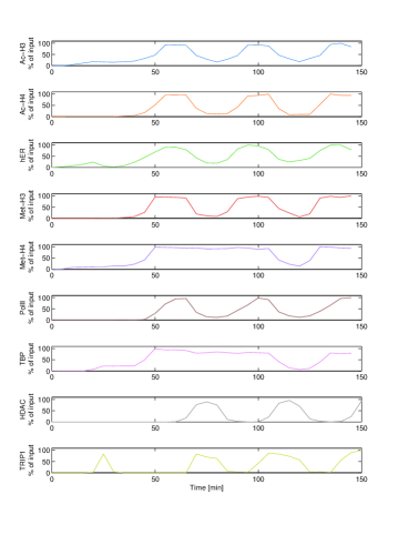
Figure 2: ChIP time-series for the pS2 promoter: The time-series show the ChIP signals (normalized) for five proteins and modifications (methylation and acetylation) of two histones. Each time-series covers the first, unproductive cycle and three productive cycles (data extracted from Métivier et al. (2003); Lemaire2006a).

4 Method

In Schölling et al. (2013) we represented the recruitment process as a walk on a network of recruitment states. Each cell traverses this network, one state after another. The waiting times $\tau$ between the state transitions from $i$ to $j$ are considered as a probabilistic event drawn from an exponential distribution

$$\rho_{ji}(\tau)=a_{ji}\exp(-a_{ji}\tau),$$ (3)

where the $a_{ji}$ determine the transition rates. In particular if no transition $i\rightarrow j$ is possible, then $a_{ji}=0$. In the case of sequential recruitment each state has only one possible successor state (compare Fig. 1). We showed that the probability of a cell to be in state $j$ is then given by Eq. (1). Since the number of cells in a ChIP experiment is large, $p_{k}(t)$ does not only represent the probability for a single cell to be in state $k$ but also estimates the probability of occupation of a state within the whole cell population at a given time.

The information of whether a protein $m$ is present in a state $k$ is represented by a matrix $S_{mk}$: If the protein is bound in state $k$ then $S_{mk}=1$ and $S_{mk}=0$ otherwise. By calculating the probability $p_{k}(t)$ of a cell to be in state $k$ at time $t$, the resulting ChIP time-series $c_{m}(t)$ can be predicted by

$$c_{m}(t)=\sum_{k=1}^{N}S_{mk}p_{k}(t)\,.$$ (4)

For a large number of recruitment states ($N\rightarrow\infty$) one obtains that the ChIP signal for a sequential recruitment process is a convolution of the protein binding pattern $S_{m}(x)$ with the initial distribution of states $P_{0}(x)$, where is constant over time ($P_{0}(x)\equiv p_{xN}(t=0)$, see Eq. (2)). Thus the ChIP signal does not directly represent the binding pattern but is “blurred” by $P_{0}(x)$.

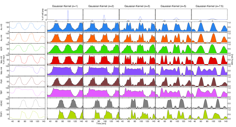
Figure 3: Results for Wiener deconvolution (5% signal-to-noise ratio, 1^st row: deconvolution kernel). 1^st column: ChIP time-series for five proteins and modifications (methylation and acetylation) of histones H3 and H4. 2^nd – 6^th column: protein binding pattern (normalized) for the deconvolution in Wiener space with Gaussian kernel with standard deviations $\sigma=\{1\,\textrm{min},2\,\textrm{min},3\,\textrm{min},5\,\textrm{min},7.5\,\textrm{min}\}$.

$P_{0}(x)$ can be identified as the convolution kernel, the $S_{m}(x)$ as the deconvoluted signal and the $c_{m}(t)$’s as the convoluted signals. One can therefore apply deconvolution methods to recover the protein binding pattern from the ChIP signal.

Deconvolution methods are frequently used in image processing where the task is to reconstruct the original image from a blurred image. From a mathematical point of view, the task is to recover the unknown, un-blurred function $g(x)\equiv S_{m}(t)$ from a known, blurred function $f(x)\equiv c_{m}(t)$ where $h(x)$ describes the blurring process. The convolution kernel $h(x)$ is unknown in many applications. To overcome this dilemma, one either has to assume a certain kernel function or use methods that are able to estimate the kernel $h(x)$ from the blurred image with the help of certain assumptions. The latter methods are called blind deconvolution methods (Fish et al., 1995; Levin et al., 2009).

In this paper we assume that the kernel is given by a Gaussian distribution, meaning that some cells are already ahead in the recruitment process whereas others lag behind. Based on the results of Métivier et al. (2003) and Schölling et al. (2013), we assume that the recruitment process is sequential and the kernel is constant in time, i.e. the de-synchronization happened prior to the considered time interval that is used for deconvolution. The latter can be justified by the fact that no obvious decay of signals is detectable in the ChIP time-series we consider (Schölling et al., 2013). Thus, no further (de-)synchronization of the cell population occurs during this time interval.

Note that the analysis of recruitment processes that are non-sequential, i.e. these processes are not traversed in a cyclic order but contain “shortcuts” or alternative recruitment pathways, is beyond the scope of this paper.

An important property of ChIP assays is their sensitivity: the unit of $c_{m}(t)$ is expressed in “percentage of input”, meaning the relative abundance of a specific DNA sequence using a protein-specific antibody compared to a non-specific antibody control. This approach leaves one degree of freedom in amplitude of the ChIP time-series since different antibodies can have different affinities and thus cause ChIP signals that differ in amplitude. Consequently, this property also transfers to the amplitude of the protein binding pattern $S_{m}(t)$. For this reason, we normalize the amplitude of ChIP time-series $c_{m}(t)$ and the protein binding pattern $S_{m}(t)$.

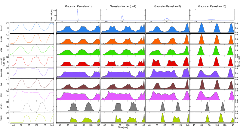
Figure 4: Results for Lucy-Richardson deconvolution (same setup as in Fig. (3)): For Gaussian kernels with small standard deviation the binding patterns do not differ strongly from the corresponding ChIP time-series. The protein binding patterns for larger Gaussian kernels show distinct peaks for the binding events. The protein binding patterns for TBP and Met-H4 show plateaus.

In this paper we consider four deconvolution methods:

• Wiener deconvolution (Dhawan1985) is a deconvolution method that works in the frequency domain. In contrast to naive deconvolution in Fourier space, it suppresses amplification of errors at frequencies with a low signal-to-noise ratio.

• The Lucy-Richardson (LR) deconvolution is a method based on Bayes’ theorem. It maximizes the likelihood of the restored signal to be the true one by using the expectation-maximization algorithm (Lucy, 1974).

• Blind Lucy-Richardson deconvolution tries to recover the convolution kernel by exploiting the commutative property of the convolution operation: With an initial guess of the kernel, the LR scheme is applied iteratively first to calculate a preliminary deconvolution of the convoluted signal and then to calculate a new kernel from this preliminary deconvolution result (Biggs and Andrews, 1997).

• Binary blind deconvolution (Lam, 2007) applies a binary constraint on the deconvoluted signal ($g(x)\in\{0,1\}$). The deconvolution can then be cast into a convex optimization problem, which can be solved by standard methods for convex optimization.

In contrast to the first two deconvolution methods the latter methods are blind deconvolution methods: These algorithms try to predict a convolution kernel $h(x)$ instead of using a given kernel as input. The problem of blind deconvolution is ill-posed in general (Levin et al., 2009): Many pairs $\{h(x),f(x)\}$ of kernel and un-blurred function exists that can reproduce the observed, blurred signal $f(x)$. Thus additional assumptions on the kernel and/or on the un-blurred signal are necessary. A detailed description of the deconvolution methods can be found in the Supporting Information.

We investigate the suitability of these four deconvolution methods to recover the protein binding pattern from ChIP signals for the pS2 gene in the next section.

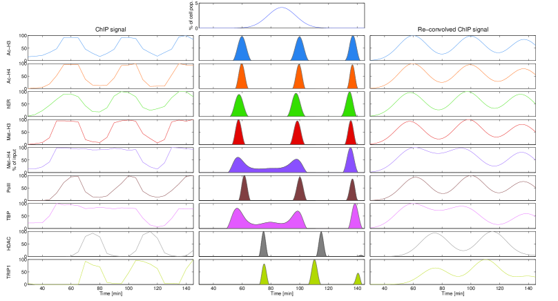
Figure 5: Results for Lucy-Richardson deconvolution with the Gaussian kernel $\sigma=9.69\textrm{min}$) ( 1^st row: deconvolution kernel). 1^st column: ChIP time-series for five proteins and modifications (methylation and acetylation) of histones H3 and H4. 2^nd–6^th column: protein binding pattern (normalized) for the Lucy-Richardson deconvolution with Gaussian kernel with standard deviations $\sigma=9.69\,\textrm{min}$. 3^rd row: result of re-convolving the deconvolved signal with the Gaussian kernel (compare to 1^st column).

5 Results

We apply the four deconvolution methods to ChIP time-series for the promoter of the pS2 gene in human MCF-7 breast cancer cells (Métivier et al., 2003). Transcription of the pS2 gene is induced by the human estrogen receptor hER$\alpha$. Here we consider the binding of five proteins (hER$\alpha$, HDAC, PolII, TBP, TRIP1) and the histone modifications (acetylation and methylation) of two histones (H3 and H4). The time-series of the ChIP data in Fig. (2) covers a time interval of 145 minutes with an experimental temporal resolution of approximately 5 minutes and exhibits oscillatory dynamics. We resampled the data to a time axis with $\Delta t=15\textrm{sec}$ to account for non-equidistributed time points. Since the first transcription cycle is unproductive, we only consider the time span 35–145min of the experiment. A striking feature of the ChIP signals in the dataset extracted from Métivier et al. (2003) is that two of the signals (Met-H4 and TBP) show distinct dynamics from the other five signals: Instead of three oscillations, only two oscillations can be observed. Note that exclusion of these two signals from our analysis does not alter the deconvolution results of the other signals.

5.1 Wiener Deconvolution

The results for Wiener deconvolution are shown in Fig. (3) for Gaussian kernels with standard deviations $\sigma\in\left\{1,2,3,5,7.5\right\}$ min. We estimate the signal-to-noise ratio to be 5%. A signal-to-noise ratio of 10% only alters the deconvolution results slightly (not shown here). For kernels with low standard deviation ($\sigma\leq 2$ min) the deconvolution results barely differ from the ChIP time-series. For larger standard deviations the deconvolution results in protein binding patterns exhibit negative amplitudes. This violates the constraint that concentrations can only be non-negative and therefore have to be discarded. The results of Wiener deconvolution show that this deconvolution method only results in valid binding patterns for Gaussian kernels with small standard deviation ($\sigma\leq 2\,$min) and these binding patterns show only marginal differences compared to the original ChIP signals.

5.2 Lucy-Richardson Deconvolution

The results of the Lucy-Richardson deconvolution method are shown in Fig. (4). The deconvolved signals for Gaussian kernels with a small standard deviation ($\sigma<10$ min) do not differ strongly from the ChIP signals. Artifacts in the form of large peaks are visible at the end of the protein binding patterns at $t=145$ min for $\sigma\in\{1\,\textrm{min},2\,\textrm{min}\}$. However, for a Gaussian kernel with large standard deviation ($\sigma=10$ min) the deconvolution results in distinct peaks for the protein binding patterns. Inbetween these two peaks the protein binding patterns decrease to zero (with the exceptions of TBP and Met-H4 as we discuss below).

Since convolution blurs the signal, we searched for the Gaussian kernel that results in the sparsest deconvolved signal. This Gaussian kernel was found at $\sigma=9.69\,\textrm{min}$ and is shown in Figs. (5, 6).

The signals that show approximately three periods in the ChIP time-series, also show three distinct binding times in the deconvolution result. The ChIP signals for methylation of H4 and binding of TBP show conceptually different dynamics than the ChIP signals of the other proteins (two oscillations instead of three oscillations). As a consequence, their binding patterns also show different characteristics than the binding patterns of the other signals: The first and the second binding events are not very distinct in time. Inbetween these two peaks the binding pattern exhibits plateaus in the affinity of about 0.2 and 0.15 (arbitrary units) for TBP and Met-H4, respectively.

5.3 Blind Lucy-Richardson Deconvolution

The results for the blind Lucy-Richardson deconvolution are shown in Fig. (7). Note that blind Lucy-Richardson deconvolution starts from an initial guess of the kernel and estimates the un-blurred signal and the convolution kernel with the maximal likelihood. We started the deconvolution with Gaussian kernels. The resulting kernels are shown in the first row of Fig. (7) indicated in red. The deconvolved signals are very similar to the original ChIP signal for all kernels. Interestingly, for initial Gaussian kernels with large standard deviation ($\sigma\geq 15\,\textrm{min}$) the initially broad kernels are always driven towards sharply peaked distributions, which explains the small effect yielded by this method.

5.4 Binary Blind Deconvolution

The deconvolution algorithm proposed by Lam (2007) performed worst: The algorithm failed to converge for the ChIP time-series for initial Gaussian kernels. For this reason, we can not present any protein binding patterns for this deconvolution method.

6 Discussion

Three of the four deconvolution algorithms we tested were able to deconvolve the protein binding patterns from the ChIP signals. However, Wiener deconvolution only producted valid binding patterns for sharp convolution kernels (small $\sigma$) and also blind Lucy-Richardson deconvolution resulted in sharp convolution kernels.

As one may expect deconvolution with these kernels does not show substantial differences to the original ChIP signals. This can be explained by the fact that these Gaussian kernels are very near to the Dirac delta function $\delta(x)$. Note that convolution of a signal with the Dirac delta function results in the very same signal again ($\left(f\otimes\delta\right)(x)=f(x)$).

Non-blind Lucy Richardson deconvolution resulted in protein binding patterns that did substantially differ from the ChIP signals. Regarding the results for the kernel that reproduces the sparsest admissible protein binding pattern ($\sigma=9.69$ min), the first events that occur in the recruitment process are binding of TBP and methylation of histone H4. However, these events are not indicated very sharply in the deconvolved signal and thus their binding times are less reliable. We defer the discussion of the deconvolution results for these events to the end of this section.

The protein binding patterns for the other four binding and histone modification events are indicated more distinctly than for Met-H4 and TBP. According to the deconvolutions in Fig. (6), the event that occurs first is the binding of hER$\alpha$. This result is consistent with prior biological knowledge, since the transcription of pS2 is known to be initiated by the binding of this estrogen receptor. Next in the recruitment process the histone H3 is methylized, which is indicated by sharp peaks in each of the three recruitment cycles. CBP is known to be capable of methylizing this histone (Wang et al., 2001). However, CBP is not included in the present experimental data and thus we cannot check whether CBP is accountable for this methylation event.

Deacetylation events of H3 and H4 follow according to the results of LR deconvolution. These events end just when the binding pattern of RNA polymerase II peaks. Interestingly, Métivier et al. (2006) defines a transcriptionally engaged pS2 promoter by the presence of Met-H4 and Ac-H3. In the results of LR deconvolution the methylation time of H4 is not indicated very precisely, but the time of deacetylation for H3 matches with the binding of RNA polymerase II.

The re-convoluted signals of HDAC and TRIP1 exhibit the largest errors in reconstructing the initial ChIP time-series (Fig. 5) and regarding to our results they bind very late in the recruitment process. It is known that these proteins are involved in promoter clearance (Métivier et al., 2003) which is in agreement with the late binding time predicted by our results. However, the predicted binding time of HDAC (histone deacetylase) does not coincide with the deacetylation of H3 and H4.

Thus we can propose two hypotheses: Either this means that HDAC does not require to bind to the protein complex to deacetylize the histones or HDAC is bound while histone deacetylation but the Lucy-Richardson prediction of the beginning of the HDAC binding time is incorrect.

In this case the binding of HDAC better coincides with the deacetylation events for kernels with small standard deviation $(\sigma\leq 2\,$min) e.g. as predicted by blind Lucy-Richardson. Thus the second possibility would indicate that cell sample used in the ChIP experiment is strongly synchronized.

We return to the discussion of Met-H4 and TBP, which show distinct dynamics in the ChIP signals: instead of three oscillations like the other time-series they only show two oscillations. Métivier et al. (2003) argued that detachment of TBP and demethylation of H4 do not occur in each productive recruitment cycle. Instead these events occur only in every second cycle. Besides the strict alternation of even and odd cycles, also probabilistic alternation is a possible interpretation of these binding patterns (Schölling et al., 2013). In this context, one can interpret the plateaus between the two peeks for TBP and Met-H4 in Figs. (4, 6) as signals only from those cells in which TBP does not detach and H4 is not de-methylized after the first productive cycle.

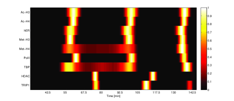
Figure 6: Results for Lucy-Richardson deconvolution with the Gaussian kernel $\sigma=9.69\,\textrm{min}$ (shows the same data as 2^nd column of Fig. 5): blue areas indicate low binding affinity, red areas indicate high binding affinities.

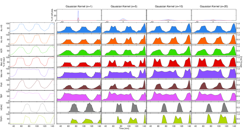
Figure 7: Results for blind Lucy-Richardson deconvolution (same setup as in Fig. 3): 1^st row: The initial kernels are plotted in blue and the final estimation of the kernels are plotted in red. For all kernels the protein binding patterns show strong similarities to the original ChIP time-series.

7 Conclusions

In the present paper, we have analyzed the applicability of different deconvolution methods to recover the protein binding pattern from ChIP time-series with an imperfectly synchronized cell population. Our analysis showed that Lucy-Richardson deconvolution can be used to improve inference on protein binding pattern from ChIP time-series. The presented results allow a more precise interpretation of the ChIP data in forms of the function proteins play in the recruiting protein complex and the recruitment process in general. We considered two non-blind deconvolution methods, Wiener deconvolution and Lucy-Richardson deconvolution, as well as two blind deconvolution methods, blind Lucy-Richardson deconvolution and binary blind deconvolution. The applicability of these methods was tested on ChIP data for the pS2 gene. Binary blind deconvolution failed to perform deconvolution. Wiener deconvolution and blind Lucy-Richardson deconvolution resulted in protein binding patterns that did not differ substantially from the original ChIP signals. For Wiener deconvolution broader convolution kernels violate the positivity constraint of the deconvoluted signal. However, the Lucy-Richardson deconvolution method has proofed its potential to recover protein binding patterns with distinct binding times. The binding pattern of HDAC indicates a late binding time which corresponds to its clearance function in the recruitment process but does not coincide with the deacetylation events of H3 and H4. This can either be interpreted as an inaccurate prediction of the proteins’ binding pattern for this deconvolution method or it means that HDAC does not require to bind to the promoter to deacetylize the histones. The reconstruction of the binding patterns succeeded for all other proteins. Their timing is in agreement with prior biological knowledge and can help to investigate the exact function of the proteins in the recruitment process.

Funding

This work has been supported by the Forum Integrativmedizin an initiative of the Hilde Umdasch Privatstiftung.

References

- Métivier et al. (2006) Raphaël Métivier, George Reid, and Frank Gannon. Transcription in four dimensions: nuclear receptor-directed initiation of gene expression. EMBO reports, 7(2):161–7, February 2006. ISSN 1469-221X. 10.1038/sj.embor.7400626. URL http://www.pubmedcentral.nih.gov/articlerender.fcgi?artid=1369254&tool=pmcentrez&rendertype=abstract.
- Hager et al. (2006) Gordon L Hager, Cem Elbi, Thomas A Johnson, Ty Voss, Akhilesh K Nagaich, R Louis Schiltz, Yi Qiu, and Sam John. Chromatin dynamics and the evolution of alternate promoter states. Chromosome research : an international journal on the molecular, supramolecular and evolutionary aspects of chromosome biology, 14(1):107–16, January 2006. ISSN 0967-3849. 10.1007/s10577-006-1030-0. URL http://www.springerlink.com/content/l628828341378037/.
- Métivier et al. (2003) Raphaël Métivier, Graziella Penot, Michael R Hübner, George Reid, Heike Brand, Martin Kos, and Frank Gannon. Estrogen receptor-alpha directs ordered, cyclical, and combinatorial recruitment of cofactors on a natural target promoter. Cell, 115(6):751–63, December 2003. ISSN 0092-8674. URL http://www.ncbi.nlm.nih.gov/pubmed/14675539.
- de Graaf et al. (2010) Petra de Graaf, Florence Mousson, Bart Geverts, Elisabeth Scheer, Laszlo Tora, Adriaan B Houtsmuller, and H Th Marc Timmers. Chromatin interaction of TATA-binding protein is dynamically regulated in human cells. Journal of cell science, 123(Pt 15):2663–71, August 2010. ISSN 1477-9137. 10.1242/jcs.064097. URL http://jcs.biologists.org/content/123/15/2663.long.
- Stasevich and McNally (2011) Timothy J Stasevich and James G McNally. Assembly of the transcription machinery: ordered and stable, random and dynamic, or both? Chromosoma, 120(6):533–45, December 2011. ISSN 1432-0886. 10.1007/s00412-011-0340-y. URL http://www.springerlink.com/content/h516204218321267/.
- Bosisio et al. (2006) Daniela Bosisio, Ivan Marazzi, Alessandra Agresti, Noriaki Shimizu, Marco E Bianchi, and Gioacchino Natoli. A hyper-dynamic equilibrium between promoter-bound and nucleoplasmic dimers controls NF-kappaB-dependent gene activity. The EMBO journal, 25(4):798–810, February 2006. ISSN 0261-4189. 10.1038/sj.emboj.7600977. URL http://www.pubmedcentral.nih.gov/articlerender.fcgi?artid=1383558&tool=pmcentrez&rendertype=abstract.
- Hager et al. (2009) Gordon L Hager, James G McNally, and Tom Misteli. Transcription dynamics. Molecular Cell, 35(6):741–53, September 2009. ISSN 1097-4164. 10.1016/j.molcel.2009.09.005. URL http://dx.doi.org/10.1016/j.molcel.2009.09.005.
- Schölling et al. (2013) Manuel Schölling, Rudolf Hanel, and Stefan Thurner. Protein complex formation: Computational clarification of the sequential versus probabilistic recruitment puzzle. In review process, 2013.
- Lee et al. (2005) David Y Lee, Catherine Teyssier, Brian D Strahl, and Michael R Stallcup. Role of protein methylation in regulation of transcription. Endocrine reviews, 26(2):147–70, April 2005. ISSN 0163-769X. 10.1210/er.2004-0008. URL http://edrv.endojournals.org/cgi/content/abstract/26/2/147.
- Kraus and Kadonaga (1998) W. L. Kraus and J. T. Kadonaga. p300 and estrogen receptor cooperatively activate transcription via differential enhancement of initiation and reinitiation. Genes & Development, 12(3):331–342, February 1998. ISSN 0890-9369. 10.1101/gad.12.3.331. URL http://genesdev.cshlp.org/content/12/3/331.short.
- Ashall et al. (2009) Louise Ashall, Caroline A Horton, David E Nelson, Pawel Paszek, Claire V Harper, Kate Sillitoe, Sheila Ryan, David G Spiller, John F Unitt, David S Broomhead, Douglas B Kell, David A Rand, Violaine Sée, and Michael R H White. Pulsatile stimulation determines timing and specificity of NF-kappaB-dependent transcription. Science (New York, N.Y.), 324(5924):242–6, April 2009. ISSN 1095-9203. 10.1126/science.1164860. URL http://www.sciencemag.org/cgi/content/abstract/324/5924/242.
- Lemaire et al. (2006) Vincent Lemaire, Chiu Lee, Jinzhi Lei, Raphaël Métivier, and Leon Glass. Sequential Recruitment and Combinatorial Assembling of Multiprotein Complexes in Transcriptional Activation. Physical Review Letters, 96(19):2–5, May 2006. ISSN 0031-9007. 10.1103/PhysRevLett.96.198102. URL http://link.aps.org/doi/10.1103/PhysRevLett.96.198102.
- Hanel et al. (2012) Rudolf Hanel, Manfred Pöchacker, Manuel Schölling, and Stefan Thurner. A self-organized model for cell-differentiation based on variations of molecular decay rates. PloS one, 7(5):e36679, January 2012. ISSN 1932-6203. 10.1371/journal.pone.0036679. URL http://www.plosone.org/article/metrics/info:doi/10.1371/journal.pone.0036679;jsessionid=99BAFC12FE5C52D421728C036B456DB5.
- Fergus et al. (2006) Rob Fergus, Barun Singh, Aaron Hertzmann, Sam T. Roweis, and William T. Freeman. Removing camera shake from a single photograph. ACM Transactions on Graphics, 25(3):787, July 2006. ISSN 07300301. 10.1145/1141911.1141956. URL http://dl.acm.org/citation.cfm?id=1141911.1141956.
- Schulz et al. (1997) Timothy Schulz, Bruce Stribling, and Jason Miller. Multiframe blind deconvolution with real data: imagery of the Hubble Space Telescope. Optics Express, 1(11):355, November 1997. ISSN 1094-4087. 10.1364/OE.1.000355. URL http://www.opticsexpress.org/abstract.cfm?URI=oe-1-11-355.
- Cannon (1976) M. Cannon. Blind deconvolution of spatially invariant image blurs with phase. IEEE Transactions on Acoustics, Speech, and Signal Processing, 24(1):58–63, February 1976. ISSN 0096-3518. 10.1109/TASSP.1976.1162770. URL http://ieeexplore.ieee.org/articleDetails.jsp?arnumber=1162770&contentType=Journals+%26+Magazines.
- McDonald et al. (2012) Geoff L. McDonald, Qing Zhao, and Ming J. Zuo. Maximum correlated Kurtosis deconvolution and application on gear tooth chip fault detection. Mechanical Systems and Signal Processing, 33(null):237–255, November 2012. ISSN 08883270. 10.1016/j.ymssp.2012.06.010. URL http://dx.doi.org/10.1016/j.ymssp.2012.06.010.
- Nadler et al. (1989) T. K. Nadler, S. T. McDaniel, M. O. Westerhaus, and J. S. Shenk. Deconvolution of Near-Infrared Spectra. Applied Spectroscopy, 43(8):1354–1358, November 1989. URL http://as.osa.org/abstract.cfm?URI=as-43-8-1354.
- Down et al. (2008) Thomas A Down, Vardhman K Rakyan, Daniel J Turner, Paul Flicek, Heng Li, Eugene Kulesha, Stefan Gräf, Nathan Johnson, Javier Herrero, Eleni M Tomazou, Natalie P Thorne, Liselotte Bäckdahl, Marlis Herberth, Kevin L Howe, David K Jackson, Marcos M Miretti, John C Marioni, Ewan Birney, Tim J P Hubbard, Richard Durbin, Simon Tavaré, and Stephan Beck. A Bayesian deconvolution strategy for immunoprecipitation-based DNA methylome analysis. Nature biotechnology, 26(7):779–85, July 2008. ISSN 1546-1696. 10.1038/nbt1414. URL http://www.pubmedcentral.nih.gov/articlerender.fcgi?artid=2644410&tool=pmcentrez&rendertype=abstract.
- Lun et al. (2009) Desmond S Lun, Ashley Sherrid, Brian Weiner, David R Sherman, and James E Galagan. A blind deconvolution approach to high-resolution mapping of transcription factor binding sites from ChIP-seq data. Genome biology, 10(12):R142, January 2009. ISSN 1465-6914. 10.1186/gb-2009-10-12-r142. URL http://genomebiology.com/2009/10/12/R142.
- Fish et al. (1995) D. A. Fish, A. M. Brinicombe, E. R. Pike, and J. G. Walker. Blind deconvolution by means of the Richardson-Lucy algorithm. Journal of the Optical Society of America A, 12(1):58, January 1995. ISSN 1084-7529. 10.1364/JOSAA.12.000058. URL http://josaa.osa.org/abstract.cfm?URI=josaa-12-1-58.
- Levin et al. (2009) A. Levin, Y. Weiss, F. Durand, and W.T. Freeman. Understanding and evaluating blind deconvolution algorithms. In 2009 IEEE Conference on Computer Vision and Pattern Recognition, pages 1964–1971. IEEE, June 2009. ISBN 978-1-4244-3992-8. 10.1109/CVPR.2009.5206815. URL http://ieeexplore.ieee.org/articleDetails.jsp?arnumber=5206815&contentType=Conference+Publications.
- Andre et al. (1979) J. C. Andre, L. M. Vincent, D. O’Connor, and W. R. Ware. Applications of fast Fourier transform to deconvolution in single photon counting. The Journal of Physical Chemistry, 83(17):2285–2294, August 1979. ISSN 0022-3654. 10.1021/j100480a021. URL http://dx.doi.org/10.1021/j100480a021.
- Lucy (1974) L. B. Lucy. An iterative technique for the rectification of observed distributions. The Astronomical Journal, 79:745, June 1974. ISSN 00046256. 10.1086/111605. URL http://adsabs.harvard.edu/abs/1974AJ.....79..745L.
- Biggs and Andrews (1997) David S. C. Biggs and Mark Andrews. Acceleration of iterative image restoration algorithms. Applied Optics, 36(8):1766, March 1997. ISSN 0003-6935. 10.1364/AO.36.001766. URL http://ao.osa.org/abstract.cfm?URI=ao-36-8-1766.
- Lam (2007) Edmund Y. Lam. Blind Bi-Level Image Restoration With Iterated Quadratic Programming. IEEE Transactions on Circuits and Systems II: Express Briefs, 54(1):52–56, January 2007. ISSN 1057-7130. 10.1109/TCSII.2006.883101. URL http://ieeexplore.ieee.org/articleDetails.jsp?arnumber=4063471&contentType=Journals+%26+Magazines.
- Wang et al. (2001) H Wang, Z Q Huang, L Xia, Q Feng, H Erdjument-Bromage, B D Strahl, S D Briggs, C D Allis, J Wong, P Tempst, and Y Zhang. Methylation of histone H4 at arginine 3 facilitating transcriptional activation by nuclear hormone receptor. Science (New York, N.Y.), 293(5531):853–7, August 2001. ISSN 0036-8075. 10.1126/science.1060781. URL http://stke.sciencemag.org/cgi/content/abstract/sci;293/5531/853.