From field theory to superfluid hydrodynamics of dense quark matter

Mark G. Alford, S. Kumar Mallavarapu
Department of Physics, Washington University St Louis, MO, 63130, USA

Andreas Schmitt, Stephan Stetina
Institute for Theoretical Physics, Vienna University of Technology, 1040 Vienna, Austria

1 Introduction

The study of quantum chromodynamics (QCD) at low temperatures and high densities is relevant for fundamental as well as applied astrophysical questions. On the fundamental side, the phase diagram of QCD at high and intermediate densities might be very complicated and its study is highly non-trivial. While heavy-ion collisions and lattice calculations are powerful tools to probe the phase structure in a regime of high temperatures and low densities, their applicability at higher densities is very limited. However, future accelerator facilities such as NICA might provide some insight (see for example Ref. [1]).

Reliable information can be obtained in a region of asymptotically high densities, where QCD behaves like a free field theory and perturbative calculations are possible. The ground state in this region of the phase diagram is a color superconductor where quarks of all color and flavor form cooper pairs which was termed color-flavor locking (CFL) [2]. Among many interesting features of CFL that could be discussed at this point, two are particularly important for the following analysis: CFL spontaneously breaks chiral symmetry which leads to an octet of Goldstone bosons and furthermore, CFL spontaneously breaks baryon conservation $U(1)_{B}$. Strictly speaking, perturbative calculations of for example the magnitude of the superconducting gap, are only valid at (rather exotic) values of the chemical potential of about $\mu\simeq 10^{8}\,{\rm MeV}$ and it is thus questionable whether CFL will persist all the way down to the phase boundary of nuclear matter. Going down in density, the increase in the mass of the strange quark will act as an external stress on the highly symmetric pairing pattern and systematic studies show [3], that CFL will most likely react by developing a kaon condensate. The corresponding ground state CFL-$K^{0}$ is then subject to two symmetry breaking patterns: The breaking of chiral symmetry and baryon conservation in CFL and the breaking of strangeness conservation due to the kaon condensate.

$$SU(3)_{L}\otimes SU(3)_{R}\otimes SU(3)_{C}\otimes U(1)_{B}\rightarrow SU(3)_{L+R+C}\otimes\mathcal{Z}_{2}\,,\,\,SU(3)_{L+R+C}\supseteq U(1)_{S}\rightarrow 1\,.$$ (1)

One should note at this point that weak interactions explicitly violate strangeness conservation and thus $U(1)_{S}$ is not an exact symmetry to begin with (we shall come back to this point in the outlook). Apart from CFL-$K^{0}$, there are many other possible candidate ground states of QCD at intermediate densities [4], but the absence of controlled experiments in laboratories or reliable models to perform calculations make it very difficult to decide which phases are realized in nature.

The study of compact stars as the only “laboratory“ where such intermediate densities are realized could prove to be very useful. The maximum value for the chemical potential inside a compact star is estimated to be high enough for deconfined quark matter to be conceivable ($\mu_{star}\leq 500\,{\rm MeV}$) . Usually, most insights into the interior of compact stars can be obtained from the characteristics of cooling and neutrino emissivity as well as from mass-radius relations. Other observable phenomena such as pulsar glitches or r-mode instabilities require a hydrodynamic description. In order to provide a framework for such calculations, it is important to understand how an effective hydrodynamic description emerges from the underlying microscopic physics discussed above. Moreover, different (equivalent) formulations of superfluid hydrodynamics exist in the literature and should be connected to each other. These were the central aims of Ref. [5] whose main results shall be reviewed here.

2 Superfluid hydrodynamics from field theory

The spontaneous breaking of a $U(1)$ symmetry, be it the breaking of $U(1)_{B}$ or $U(1)_{S}$ discussed above, is known to be the fundamental mechanism for superfluidity. We will focus here on kaon condensation (and thus on the breaking of $U(1)_{S}$), but similar considerations hold for essentially any system with a spontaneously broken symmetry. The existence of a condensate together with the absence of elementary excitations which could dissipate energy allow for frictionless transport of the associated $U(1)_{S}$ charge at low temperatures. This might be puzzling at first since it is also well known that the spontaneous breaking of a global symmetry leads to existence of massless excitations (Goldstone bosons). At least at zero temperature, this apparent contradiction can easily be resolved: since the low-energy dispersion relation of the Goldstone mode is linear in momentum, it can only be excited beyond a certain critical velocity which is given by the slope of the linear part of the dispersion. At nonzero temperature, the situation is more complicated as thermal excitations of the Goldstone mode (“phonons”) are present for any superfluid velocity. As a consequence, in the translation into hydrodynamic equations, we will have to consider both ingredients, condensate and phonons, and they also appear coupled to each other.

The hydrodynamic framework capable of describing superfluids, which we will derive now from microscopic physics, was first set up by Landau [6] mainly for the (non-relativistic) purpose of describing superfluid helium. The basic idea is to formally divide the fluid into a superfluid and normal fluid part. The total mass density (later in the relativistic context to be replaced by charge density) is then given by $\rho=\rho_{n}+\rho_{s}$ where at zero temperature only the superfluid density is present and above the critical temperature only the normal fluid density. From this point of view, the hydrodynamic description of CFL with kaon condensation is quite complex: due to the breaking of $U(1)_{B}$ and $U(1)_{S}$ two superfluid components are present such that in total we expect to be dealing with four different fluid components. In order to derive the two component hydrodynamics for the kaon part, we start by analyzing a complex scalar $\varphi^{4}$ model, which can be interpreted as an effective theory for kaons [7].

2.1 Zero temperature

Based on Ref. [8], we start with our derivation at zero temperature, where only the superfluid component is present. As mentioned at the end of the last section, our starting point will be a $\varphi^{4}$ theory where the complex doublet field can be interpreted as $(\varphi,\varphi^{*})=(K_{0},\overline{K}_{0})$:

$$\mathcal{L}=\partial_{\mu}\varphi\partial^{\mu}\varphi^{*}-m^{2}\left|\varphi\right|^{2}-\lambda\left|\varphi\right|^{4}\,\,.$$ (2)

After introducing the condensate,

$${\displaystyle\varphi\rightarrow\left\langle\varphi\right\rangle+{\rm fluctuations}\,,\qquad\left\langle\varphi\right\rangle=\frac{\rho(x)}{\sqrt{2}}e^{i\psi(x)}}\,\,,$$ (3)

we simplify calculations by additionally assuming a constant modulus $\rho$ of the condensate. The equations of motion then imply [5] that also $\partial^{\mu}\psi$ is constant and the tree-level potential turns into:

$$U\equiv-\mathcal{L}=-\frac{(\sigma^{2}-m^{2})^{2}}{4\lambda}\,\,,\,\,\,\,\,\,\,\,\,\,\,\,\,\sigma\equiv\sqrt{\partial_{\mu}\psi\partial^{\mu}\psi}\,\,.$$ (4)

Field-theoretic definitions for the Noether current and stress energy tensor can be matched to the corresponding hydrodynamic expressions:

$$j^{\mu} = n_{s}v_{s}^{\mu}=\frac{\partial\mathcal{L}}{\partial(\partial_{\mu}\psi)}=\partial^{\mu}\psi\frac{\sigma^{2}-m^{2}}{\lambda}\,\,,$$ (5)

$$T^{\mu\nu} = (\epsilon_{s}+P_{s})v_{s}^{\mu}v_{s}^{\nu}-g^{\mu\nu}P_{s}=\frac{2}{\sqrt{-g}}\frac{\delta\left(\sqrt{-g}\mathcal{L}\right)}{\delta g_{\mu\nu}}=\partial^{\mu}\psi\partial^{\nu}\psi\frac{\sigma^{2}-m^{2}}{\lambda}-g^{\mu\nu}\mathcal{L}\,\,.$$ (6)

Charge density $n_{s}$ and the flow velocity of the superfluid $v_{s}^{\mu}$ can than easily be obtained:

$$n_{s}=\sqrt{j_{\mu}j^{\mu}}=\sigma\frac{\sigma^{2}-m^{2}}{\lambda}\,\,,\,\,\,\,\,\,\,\,\,\,\,\,v_{s}^{\mu}=\frac{\partial^{\mu}\psi}{\sigma}\,\,,$$ (7)

as can be energy and pressure density of the superfluid ($\epsilon_{s}$ and $P_{s}$) by making use of proper projections on $T^{\mu\nu}$. It is important to notice that our simplification of $\partial^{\mu}\psi$ being constant translates into a uniform superflow velocity. Finally we include thermodynamics into our considerations which allows us to identify the chemical potential in the superfluid rest frame, $\mu_{s}=\sigma$. The Lorentz invariant quantity $\sigma$ can also be expressed in terms of the chemical potential in the normal-fluid rest frame $\mu=\partial_{0}\psi$: with the above definition of the superfluid velocity, a usual Lorentz factor arises in this relation,

$$\sigma=\mu\sqrt{1-\vec{v}_{s}^{2}}\,\,.$$ (8)

As we can see, both chemical potential and flow velocity of the superfluid evolve solely from rotations of the phase of the condensate: rotations of the phase around the U(1) circle per unit time create the chemical potential and the rotations per unit length gives rise to the superflow velocity.

2.2 Finite temperature

In order to introduce finite temperature $T$, we use the simple one-loop effective action with the tree-level potential $U$ as introduced before and the inverse propagator $S^{-1}$:

$$\Gamma=-\frac{V}{T}U-\frac{1}{2}\sum_{k}{\rm Tr}\ln\frac{S^{-1}(k)}{T^{2}},\,\,\,\,\,\,\,\,\,\,\,S^{-1}(k)=\left(\begin{array}[]{cc}-k^{2}+2(\sigma^{2}-m^{2})&2ik\cdot\partial\psi\\ -2ik\cdot\partial\psi&-k^{2}\end{array}\right)\,.$$ (9)

We work at small coupling $\lambda\ll 1$ and restrict ourselves to small temperatures (much below the critical temperature and $T\ll\mu$). Furthermore, any temperature dependence of the condensate $\rho$ has been neglected. These approximations allow us to obtain analytic results (generalizations are discussed in the outlook). Finite-temperature calculations are carried out in the Matsubara formalism, i.e. $k=(k_{0},\vec{k})$, $k_{0}=-i\omega_{n}$ with bosonic Matsubara frequencies $\omega_{n}=2\pi nT$. For small momenta, the dispersion of the Goldstone mode obtained from the poles of the propagator can be written as:

$$\epsilon_{\vec{k}}=c_{1}(x)|\vec{k}|+\frac{c_{2}(x)}{\mu^{2}}|\vec{k}|^{3}+...\,,$$ (10)

and obviously depend on $x=\cos\vartheta$ where $\vartheta$ is the angle in between $\vec{k}$ and the homogeneous background superflow $\vec{v}_{s}$. For explicit results for $c_{1}$ and $c_{2}$ please refer to Ref. [5].

At finite temperature, a hydrodynamic interpretation of field-theoretic results is much more challenging. We now have to introduce an additional “normal” current related to the elementary excitations which automatically complicates thermodynamics: since our two homogeneous flows imply two rest frames where either the normal or the super current is vanishing, it is impossible to define a frame where the pressure is isotropic. We rather have to deal with pressure densities normal and longitudinal to the non vanishing current ($T_{\perp}$,$T_{\parallel}$) in the respective rest frame, but which pressure is the correct one to appear in the thermodynamic relation?

2.2.1 Generalized thermodynamics and entrainment

The most rigorous answer to this question is contained in the canonical formalism introduced by Carter [9] which provides an extension of usual thermodynamics by making use of a generalized pressure $\Psi$ and a generalized energy density $\Lambda$. The set of variables in this framework differs from the one used in the two-fluid formalism of Landau: instead of formally dividing the Noether current into normal and supercurrent, the canonical framework is based on either the conserved charge and entropy currents $j^{\mu}$ and $s^{\mu}$ (the latter is conserved only in the non-dissipative case) or their thermodynamically conjugate momenta $\partial^{\mu}\psi$ and $\theta^{\mu}$. Lorentz covariance requires $\Lambda$ and $\Psi$ to be functionals of invariants only (i.e. $\Lambda=\Lambda[j^{2},s^{2},j_{\mu}s^{\mu}],\,\,\Psi=\Psi[\sigma^{2},\theta^{2},\partial_{\mu}\psi\theta^{\mu}]$) . Here the definition of $\sigma$ from above has been used. The relation of $\partial^{\mu}\psi$ to the chemical potential has already been discussed in the previous section and as we show later, $\theta^{\mu}$ can be related to the temperature. It might seem puzzling at first to generalize scalar quantities such as temperature to a four-vector, but the actually measured temperature is of course obtained by contraction with the velocity four-vector pointing to the rest frame of interest. We can now obtain the correct equations of motion by varying either the generalized energy density with respect to the conserved currents or the generalized pressure with respect to the conjugated momenta:

$$d\Lambda=\partial_{\mu}\psi dj^{\mu}+\theta_{\mu}ds^{\mu}\,\,,\,\,\,\,\,\,\,\,\,\,\,d\Psi=j_{\mu}d(\partial^{\mu}\psi)+s_{\mu}d\theta^{\mu}\,\,.$$ (11)

Switching between these two descriptions is identical to a change from a Hamiltonian to a Lagrangian framework, $\Lambda$ and $\Psi$ are connected by a Legendre transformation. With all these ingredients at hand, we can now write down a generalized thermodynamic relation:

$$\Lambda+\Psi=j\cdot\partial\psi+s\cdot\theta\,\,.$$ (12)

Applying the chain rule to Eq. (11) allows us to write:

$$\partial^{\mu}\psi=\frac{\partial\Lambda}{\partial j_{\mu}}={\cal B}j^{\mu}+{\cal A}s^{\mu}\,\,,\,\,\,\,\,\theta^{\mu}=\frac{\partial\Lambda}{\partial s_{\mu}}={\cal A}j^{\mu}+Cs^{\mu}\,\,,$$ (13)

with

$${\cal A}=\frac{\partial\Lambda}{\partial(j\cdot s)}\,\,,\,\,\,\,\,{\cal B}=2\frac{\partial\Lambda}{\partial j^{2}}\,\,,\,\,\,\,\,\,{\cal C}=2\frac{\partial\Lambda}{\partial s^{2}}\,\,.$$ (14)

The coefficient ${\cal A}$ appears in the relations for $\partial^{\mu}\psi$ as well as $\theta^{\mu}$. It is called “entrainment coefficient” which reflects the fact that any change in either of the two conjugate momenta will automatically affect both currents (and the other way around) such that the currents are coupled to each other. Finally, the stress-energy tensor is now given by

$$T^{\mu\nu}=-g^{\mu\nu}\Psi+j^{\mu}\partial^{\nu}\psi+s^{\mu}\theta^{\nu}\,\,.$$ (15)

Plugging in Eqs. (13), one can see right away that $T^{\mu\nu}$ becomes symmetric in the Lorentz indices.

It remains to relate the canonical formalism to the original two fluid picture of Landau (a relativistic generalization of which can for example be found in [10, 11]). After introducing a normal-fluid current, the straightforward extension of our zero-temperature expressions for Noether current and stress-energy tensor are

$${\displaystyle T^{\mu\nu}} = {\displaystyle\left(\epsilon_{n}+P_{n}\right)u_{n}^{\mu}u_{n}^{\nu}+\left(\epsilon_{s}+P_{s}\right)\partial^{\mu}\psi\partial^{\nu}\psi/\sigma^{2}+(P_{n}+P_{s})g^{\mu\nu}\,\,,}$$ (16)

$${\displaystyle j^{\mu}} = {\displaystyle n_{n}u_{n}^{\mu}+n_{s}\partial^{\mu}\psi/\sigma\,\,.}$$ (17)

Here, we have introduced the flow velocity of the normal fluid $u_{n}^{\mu}$, as well as the corresponding energy and pressure densities $\epsilon_{n}$ and $P_{n}$. The superfluid velocity is still given by Eq. (7) . The coefficients ${\cal A},\,{\cal B}$ and ${\cal C}$ prove to be very useful in translating one formalism into the other as all hydrodynamic parameters in either model can be expressed in terms of them:

$$n_{s}=\frac{\sigma}{{\cal B}}\,,\,\,\,\,\,\,n_{n}=-\frac{{\cal A}}{{\cal B}}s,\,\,\,\,\,\,\epsilon_{s}+P_{s}=\frac{\sigma^{2}}{{\cal B}},\,\,\,\,\,\,\epsilon_{n}+P_{n}=\frac{{\cal B}{\cal C}-{\cal A}^{2}}{{\cal B}}s^{2}\,\,.$$ (18)

Note that in (16) and (17) $j^{\mu}$ and at the same time $\partial^{\mu}\psi$ appear as parameters such that in the strict sense of the canonical framework, this has to be considered a “mixed” form.

2.2.2 Explicit results at finite temperature

In the terminology of the Landau formalism, it can be shown [5] that all microscopic calculations at finite temperature are carried out in the normal fluid rest frame where we can identify generalized pressure $\Psi$ and temperature:

$$\Psi=\frac{T}{V}\Gamma\,,\,\,\,\,\,\,\,\,\,\,\,\,\,\theta_{0}=T\,\,\,\,\,\,\,\,\,\,\,\,\,\mbox{in the normal fluid rest frame.}$$ (19)

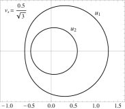
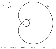
Figure 1: Velocities of first and second sound $u_{1}$ and $u_{2}$. The homogeneous background superflow is aligned along the horizontal axis and the speeds of sound are calculated for all angles with respect to the superflow.

Even though the first relation is in principle frame independent, using our microscopic expression (9) automatically restricts us to the normal rest frame. We can now step by step derive field-theoretic definitions for all the basic quantities of the two-fluid formalism. The coefficients ${\cal A},\,{\cal B}$ and ${\cal C}$ are in terms of microscopic variables

$${\cal A}=\frac{\partial^{0}\psi}{s^{0}\vec{j}\cdot\vec{\nabla}\psi}\eta\,\,,\,\,\,\,\,\,{\cal B}=-\frac{(\vec{\nabla}\psi)^{2}}{\vec{j}\cdot\vec{\nabla}\psi}\,\,,\,\,\,\,\,\,{\cal C}=-\frac{j^{0}\partial^{0}\psi\,\eta-\vec{j}\cdot\vec{\nabla}\psi s^{0}\theta^{0}}{(s^{0})^{2}\vec{j}\cdot\vec{\nabla}\psi\,\,,}$$ (20)

with the abbreviation $\eta=\vec{v}_{s}^{2}j^{0}\partial^{0}\psi+\vec{j}\cdot\vec{\nabla}\psi$. With the help of these, we can easily obtain explicit results of for example the normal-fluid density in the low-temperature limit,

$$n_{n}\simeq\frac{4\pi^{2}}{5\sqrt{3}}\frac{T^{4}}{\mu}\frac{(1-\vec{v}_{s}^{2})^{2}}{(1-3\vec{v}_{s}^{2})^{3}}-\frac{48\pi^{4}}{7\sqrt{3}}\frac{T^{6}}{\mu^{3}}\frac{(1-\vec{v}_{s}^{2})^{2}}{(1-3\vec{v}_{s}^{2})^{6}}\left(15+38\vec{v}_{s}^{2}-9\vec{v}_{s}^{4}\right)\,\,.$$ (21)

As it turns out, the normal fluid density is not just the phonon contribution to the number density which would yield a $T^{3}$ rather than $T^{4}/\mu$ contribution.

Finally, as an application we present the velocities of first and second sound in the background of the superflow. The complete calculation is lengthy and can be found in the appendix of Ref. [5]. The final results for $T=0$ are shown in Fig. 1. The sound velocities depend on the angle between the direction of the sound wave and the direction of the superflow. The velocity of second sound decreases significantly as the superflow approaches its critical velocity $v_{crit}=1/\sqrt{3}$. The impact of small temperature corrections on the speeds of sound is also discussed in Ref. [5].

3 Outlook

For the sake of obtaining analytic results, simplifications were made at several points. This was a necessary and important first step to gain an understanding of how superfluid hydrodynamics emerge from the underlying microscopic physics. Restriction to a low-temperature regime can be overcome by making use of the two-particle irreducible effective action [7, 12]. All hydrodynamic parameters can then be calculated numerically up to the critical temperature (and beyond) and the temperature dependence of the condensate can be taken into account. Furthermore the explicit breaking of $U(1)_{S}$ due to weak interactions can be taken into account by adding a small symmetry breaking term to the Lagrangian.

Acknowledgements: This work has been supported by the Austrian science foundation FWF under project no. P23536-N16 and by U.S. Department of Energy under contract #DE-FG02-05ER41375, and by the DoE Topical Collaboration “Neutrinos and Nucleosynthesis in Hot and Dense Matter”, contract #DE-SC0004955. I thank the organizers for giving me the opportunity to present my work in the frame of this inspiring conference.

References

- [1] A Schmitt, http://theor.jinr.ru/twiki/pub/NICA/NICAWhitePaper/Schmitt_wp8.pdf
- [2] M. G. Alford, K. Rajagopal and F. Wilczek, Nucl. Phys. B 537, 443 (1999) [hep-ph/9804403].
- [3] P. F. Bedaque and T. Schäfer, Nucl. Phys. A 697, 802 (2002) [hep-ph/0105150].
- [4] M. G. Alford, A. Schmitt, K. Rajagopal and T. Schäfer, Rev. Mod. Phys. 80, 1455 (2008) [arXiv:0709.4635 [hep-ph]].
- [5] M. G. Alford, S. K. Mallavarapu, A. Schmitt and S. Stetina, Phys. Rev. D 87, 065001 (2013) [arXiv:1212.0670 [hep-ph]].
- [6] L. Landau, Phys. Rev. 60, 356 (1941).
- [7] M. G. Alford, M. Braby and A. Schmitt, J. Phys. G 35, 025002 (2008) [arXiv:0707.2389 [nucl-th]].
- [8] D. T. Son (2002), hep-ph/0204199.
- [9] B. Carter, in Relativistic Fluid Dynamics (Noto 1987), edited by A. Anile and M. Choquet Bruhat, Springer-Verlag, 1989, pp. 1-64.
- [10] I. M. Khalatnikov and V. V. Lebedev, Physics Letters A 91, 70 (1982).
- [11] C. P. Herzog, P. K. Kovtun and D. T. Son, Phys. Rev. D 79, 066002 (2009) [arXiv:0809.4870 [hep-th]].
- [12] J.M. Cornwall, R. Jackiw, E. Tomboulis, Phys. Rev. D 10, 2428 (1974).