A GEMM interface and implementation on NVIDIA GPUs for multiple small matrices

Abstract

We present an interface and an implementation of the General Matrix Multiply (GEMM) routine for multiple small matrices processed simultaneously on NVIDIA graphics processing units (GPUs). We focus on matrix sizes under 16. The implementation can be easily extended to larger sizes. For single precision matrices, our implementation is 30% to 600% faster than the batched cuBLAS implementation distributed in the CUDA Toolkit 5.0 on NVIDIA Tesla K20c. For example, we obtain 104 GFlop/s and 216 GFlop/s when multiplying 100,000 independent matrix pairs of size 10 and 16, respectively. Similar improvement in performance is obtained for other sizes, in single and double precision for real and complex types, and when the number of matrices is smaller. Apart from our implementation, our different function interface also plays an important role in the improved performance. Applications of this software include Finite Element computation on GPUs.

1 Introduction

Implementations of the General Matrix Multiply (GEMM) routine typically achieve a large fraction of peak speed on modern multi-core hardware. However, because of hardware characteristics, high performance is achieved for large matrix sizes, which is usually in hundreds or even thousands [1, 2], or for sizes that are integer multiples of hardware-specific dimensions.

Although such large dense matrices are important in many applications and also help in showcasing the impressive speeds, many applications require multiplication of multiple independent small matrices, each having identical size. Such a situation is common in finite element methods for example [3, 4, 5, 6, 7, 8]. Even if sizes are different, one can partition matrices so that sets with identical matrix sizes are obtained.

Our goal is to obtain high performance when processing multiple small matrices on NVIDIA GPUs, numbering in thousands or much higher. The definition of small is not standard and cannot be invariant with respect to hardware trends. Still, ‘small’ can be taken to be a size for which high performance is difficult to achieve in a parallel environment unless multiple independent matrices are involved. Note that even for large matrices, efficient implementations of GEMM multiply sub-blocks which are smaller and achieve high performance. However, the difference here is that our small matrices are independent and are of different sizes.

Achieving high performance GEMM for small matrix sizes, when compared to large sizes, is inherently difficult because each entry is used fewer times after it is copied from main memory to registers. However, developing a high-quality GEMM implementation is crucial. Apart from its inherent utility, fast GEMM is also a basis for the speeds achievable in other level-3 BLAS functions [9].

In the context of GPUs, the need for a capability to multiply pairs of small matrices was recognized by NVIDIA. An implementation focused on small matrix sizes was released with the Compute Unified Device Architecture (CUDA) toolkit version 4.1 in the cuBLAS library. The so-called “batched” implementation (function name cublasXgemmBatched, X = S/D/C/Z for different data types) is significantly faster than two other possibilities – one using CUDA streams and the original non-streamed version intended for large matrices. This improvement in speed due to batching holds for matrix sizes up to roughly 100. However, except for small matrices with sizes that are integral multiples of 16, the achieved performance is still a small fraction of peak GPU speed [10]. One can also observe that the function’s performance is quite sensitive to the matrix size being a multiple of 16. For example, its speed in multiplying 100,000 single precision matrix pairs of size 16 is 134 GFlop/s. But it drops to 105 GFlops/ for size 15, and for size 17 it drops even more to 32 GFlop/s. These numbers are using the “batchCUBLAS” example program run on Tesla K20c, a device for which the peak single precision speed is 3.52 TFlop/s.

Another issue is that the function interface of cublasXgemmBatched is designed around pointers to the matrix pointers, which increases its applicability when calling from languages that can deal with pointers to pointers and if different matrices were allocated separately. But this feature also makes it less efficient because one has to transfer each pointer as extra data.

Our objectives in this contribution are to achieve higher performance GEMM for small matrices on GPUs and also to provide an alternative interface that uses a second-level leading dimension (a BLAS/LAPACK terminology [11]). Using our interface and the implementation, we achieve an improvement in speed that varies in [30%,600%] compared to the reference cuBLAS batched implementation for single precision matrices. The improvement is in the higher range when the matrix sizes are smaller. Similar improvements are observed for other scalar types.

If we just use the cuBLAS-like interface but the underlying implementation is ours, the speedup is lower but still significant. In this case, compared to the reference, we achieve a more modest speed improvement (or a minor reduction in a tiny fraction of cases) in [-30%,300%]. We also include discussion of a few C++ template related features that help in achieving generality and high performance.

Our focus here is on square matrices of size 16 or less but the method can be easily implemented for rectangular cases and for larger sizes. The main reason we have focused our attention on matrices of size 16 and less is that such sizes correspond to the polynomial degrees that are traditionally used in high-order finite elements [3, 4, 5, 6, 7, 8].

Here is an outline of the paper. In Section 2 we briefly describe our notation for batched GEMM. Sections 3 and 4 are devoted to describing the cuBLAS interface that we use as reference and the design trade-offs associated with it. In Sections 5 and  6 we describe the interface of our CUDA kernel and the function wrapping it. There we also describe various optimization possible due to C++ features. We give an overview of our implementation in Section 7. We discuss the performance of our implementation from various viewpoints in Section 8.

2 Multiple GEMMs

Let $op$ (standing for operation) refer to a mapping from matrices to matrices, such that $op(A)=A$ or $A^{T}$ or $A^{*}$ depending on an extra variable that can contain three values. The superscripts $T$ and $*$ stand for transpose and Hermitian-transpose, respectively. Consider real or complex matrices $A^{p},B^{p},C^{p}$ for $p=1,2,\ldots,N$. Here $N$ stands for the batch size. The matrices can be stored in single precision or double precision. Using the BLAS notation, $C$ is $m\times n$, $op(A)$ is $m\times k$, and $op(B)$ is $k\times n$.

Let $\alpha$ and $\beta$ be given scalars. Our goal is to compute

$$C^{p}\leftarrow\alpha\,op(A^{p})op(B^{p})+\beta\,C^{p}$$ (1)

for $p=1,2,\ldots,N$ independently in the CUDA environment. Note that in this context the operation $op$ acting on $A$ can be different than the one acting on $B$, which leads to 9 combinations in all.

3 NVIDIA cuBLAS interface

We first provide a few details of our baseline. The batched implementation in NVIDIA cuBLAS versions 4.1, 4.2, and 5.0 for computing the output in Equation (1) is a C function with a signature given below. The letter $T$ (standing for type) refers to the concrete type, which can be S,D,C,Z for float, double, cuComplex, or cuDoubleComplex respectively. The detailed documentation is available online [10]. However, the interface is easy to understand and almost natural for a BLAS/LAPACK user. The comments after // are our own.

cublasStatus_t cublasTgemmBatched(
  cublasHandle_t handle,    // library context
  cublasOperation_t transa, // CUBLAS_OP_[NTC] for A, A^T, A^*
  cublasOperation_t transb, // CUBLAS_OP_[NTC] for B, B^T, B^*
  int m, int n, int k,      // matrix sizes, discussed earlier
  const T *alpha,    // host or device pointer
  const T *Aarray[], // device pointers to 0,0 elements of A’s
  int lda,           // leading dimension of A’s
  const T *Barray[], // device pointers to 0,0 elements of B’s
  int ldb,           // leading dimension of B’s
  const T *beta,     // host or device pointer to beta
  T *Carray[],       // device pointers to 0,0 elements of C’s
  int ldc,           // leading dimension of C’s
  int batchCount);   // number of A’s, B’s, and C’s

4 Design trade-offs in the cuBLAS interface

The cuBLAS interface is natural when using multiple matrices that may have been created and stored independently or if the number of matrices is dynamically changing. However, the interface has a few design issues.

First, one would have to collect the pointers to the matrices and copy the three arrays (for $A,B,C$) to the device. Although natural for independently allocated matrices, this leads to additional overhead in transmission as well as memory access during kernel execution. Secondly, when batch size is large, say a few thousands or more, one would reduce the effective performance by spending time in allocating and deallocating a large number of independent matrices and transferring the arrays of pointers.

An alternative way to use the cuBLAS interface is to allocate a large chunk of memory once, and store pointers to appropriate positions so that it looks like a 3-D array – a uniformly-offset collection of matrices of identical size. This strategy will avoid number of allocations and deallocations to grow with $N$, the batch size. However, even now, neither the function invocation nor the kernel execution have used the knowledge that the matrices are uniformly-offset. This leads us to the hypothesis that a somewhat less general but a more efficient as well as appropriate way is to not pass pointers to pointers, but use a second leading dimension to indicate the offset between adjacent matrices. One needs to pass pointer to the 0,0 element of only the first matrix and just a single extra integer for another leading dimension.

To test this hypothesis, we will show results from two versions of our kernel, one with the interface like the one in cuBLAS and other with the 3-D array interface. In both cases, the implementation is be identical as far as logically possible. It will be shown that the second one increases performance even after transmission overhead associated with creating and passing pointers to pointers is ignored (see  Section 8). Hence, we can conclude the following based on our argument and evidence. In the regime of large batch size and small matrix sizes (less than or equal to 16), the natural interface is the one that uses a 3-D array to represent a collection of 2-D matrices.

5 A specialized function interface

As mentioned earlier, we develop kernels with two kinds of interfaces to test which interface gives us the better performance. The first one resembles the cuBLAS interface. We call it TGEMM_multi_nounif, where ‘multi’ stands for multiple and ‘nounif’ is for ‘not uniform’. The second one is called TGEMM_multi_uniform and is the focus of this research. It uses a second-level leading dimension. Hence we show the second and new interface only.

cudaError_t TGEMM_multi_uniform(
  char transa,       // [nN], [tT], [cC] for A, A^T, A^*
  char transb,       // [nN], [tT], [cC] for B, B^T, B^*
  int m, int n, int k, // matrix sizes, discussed earlier
  const T *alpha,    // host or device pointer
  const T *A3D,      // device pointer to 0,0,0 element of A’s
  int lda,           // leading dimension of each 2D A
  int lda2,          // offset between 2D A’s
  const T *B3D,      // device pointer to 0,0,0 element of B’s
  int ldb,           // leading dimension of each 2D B
  int ldb2,          // offset between 2D B’s
  const T *beta,     // host or device pointer to beta
  T *C3D,            // device pointer to 0,0,0 element of C’s
  int ldc,           // leading dimension of each 2D C
  int ldc2,          // offset between 2D C’s
  int batchCount);   // number of A’s, B’s, and C’s

The second leading dimension is the offset between adjacent 2D matrices. The $(i,j)$ entry in $k^{th}$ $A$ matrix in the batch is $A[i+lda*j+lda2*k]$. Similar relations hold for $B$ and $C$. Figure 1 shows the layout of the batch of $C$ matrices.

The “physical unit” of leading dimension is an important issue when writing code using CUDA and can be a cause of bugs if mishandled. The units of leading dimensions, both the original one and new one, are not bytes. The units are number of scalar elements. This has to be translated when interfacing with CUDA functions that work with bytes.

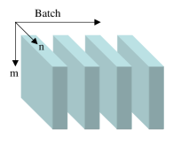
Figure 1: A layout of matrices in the TGEMM_multi_uniform kernel. The dimensions $m$ and $n$ refer to the output matrices $C^{p}$. We have $ldc\geq m$ and $ldc2\geq ldc*n$.

6 A C++ kernel interface

We now present the C++ interface for the CUDA kernel underlying the TGEMM_multi_uniform function. It is intended for multiplication of square matrices. Because of templates, it can be called by C++ code only. However, the C++ caller code can be wrapped by passing appropriate arguments so it can be called by a C function in the usual manner.

template
<
    typename T,         // single/double real/complex
    unsigned int m,     // size m = n = k
    bool transa,        // true if transposing A, else false
    bool transb,        // true if transposing B, else false
    typename unary_a,   // functor for conjugating A or not
    typename unary_b,   // functor for conjugating B or not
    typename axpby_type // functor for y <- a*x + b*y
>
__global__ void TGEMM_multi_uniform_kernel(
    const T* A,                 // A data
    unsigned int lda, int lda2, // A LDA 1 and 2
    const T* B,                 // B data
    unsigned int ldb, int ldb2, // B LDA 1 and 2
          T* C,                 // C data
    unsigned int ldc, int ldc2, // C LDA 1 and 2
    unsigned int batch_count,   // Number of A,B,C
    unary_a func_a,   // functor for conjugating A or not
    unary_b func_b,   // functor for conjugating B or not
    axpby_type axpby) // functor for y <- a*x + b*y

A C++ functor (or function object) is useful for compile-time polymorphism [12] and is important for achieving high-performance. The essential idea is to move Boolean checks from the innermost loop to outside so it will lead to fewer branching possibilities. The drawback is that it leads to larger executable code size when a large number of independent template permutations are instantiated. Of course, if only one or few instantiations are used, then one gets high performance without increasing code size significantly.

Note that our intent is not at all to suggest that cuBLAS or other libraries do not internally use functors or templates like these. Based on the cuBLAS interface, the only knowledge we have is that it uses pointers to matrices rather than second-order leading dimension. It may still be designed using such functors or templates internally.

We briefly discuss the specific rationale and a few candidates for the axpby_type and unary_a argument types. These functors are applied entry-wise to pairs of scalars. In many cases, the GEMM parameters $\alpha$ (for $a$) and $\beta$ (for $b$) are not arbitrary scalars but are simple values like -1, 0 or 1. In such cases explicit multiplication is not needed. For example, one may just want to compute $C\leftarrow AB$ (so $\alpha=1,\beta=0$). The effect on performance can be noticeable large when $\beta$ is zero but a general code still reads the output entry from global memory, multiplies it by $\beta$, and then writes the final sum back to global memory. Such extra computation and memory movement can be prevented by passing a stateless object of the following type.

template<typename T>
struct axpby_a1b0 // For a = 1, b = 0
{
    __host__ __device__
    void operator()(T& y, const T& x) const
    {
        y = x;
    }
};

The following functor can be used for general $a$ and $b$.

template<typename T>
struct axpby // For general a and b
{
    T a, b;
    axpby(const T& a, const T& b)
      : a(a), b(b)
    {}
    __host__ __device__
    void operator()(T& y, const T& x) const
    {
        y = a * x + b * y;
    }
};

One would then call axpby(C_entry, (AB)_entry) in the CUDA kernel for each entry. Functors for other special combinations of $a$ and $b$ can also be used. Note that these functors are reusable for other BLAS routines, on GPUs and CPUs alike, and are a minor coding overhead at worst and significant performance boost in general. Compiler optimizations inline all these calls.

In a similar vein, when one wants to apply conjugates for complex scalars, functors can be used that return the conjugate of a given entry. Here is an example for double precision complex.

struct conjugate_cuDoubleComplex
{
    __host__ __device__
    cuDoubleComplex operator()(const cuDoubleComplex& a) const
    {
        cuDoubleComplex a_conj = {a.x, -a.y};
        return a_conj;
    }
};

The following functor is used when conjugate is not needed.

template<typename T>
struct identity // for identity transform
{
    __host__ __device__
    T operator()(const T& a) const
    {
        return a;
    }
};

7 CUDA kernel implementation overview

We give a description of the TGEMM_multi_uniform_kernel implementation. In reality, we have two distinct methods. The first one is for matrix sizes 1-16. The second can be used for matrices where the square matrix dimension can be factorized into a product of two nearly equal numbers. For example, 15 can be factorized as $3\times 5$ or $5\times 3$. The order is important. Experimentally, we saw that the second method is faster than the first one for sizes 15 and 16 and we use that to show the results. In both methods, each CUDA thread-block is used to process multiple matrices.

In the first method, each thread within a thread-block computes one entry of output matrix $C$. All the threads read the corresponding $A$ and $B$ matrix to shared memory. Thus, for processing $m\times m$ matrices we launch $m^{2}$ threads.

In the second implementation, each thread can be used to read multiple entries of $A$ and $B$ into the shared memory. This kernel is inspired from the one implemented in MAGMA [1]. We factorize $m=m_{1}m_{2}$ and launch thread-blocks of size $(m_{1}m_{2})\times m_{2}$. Then each block has to read multiple columns of $A$ and $B$.

We use 2000 thread-blocks. This parameter can be tuned for minor additional gains for specific situations (see Figure 3). The gains will not be large unless the hardware is quite different. For matrices that are not square, one can use these square matrix kernels to multiply sub-blocks.

Another important point to note is that one can design more specialized kernels of a given matrix size so that the performance can be improved even more. However, we have not pursued this task further.

8 Performance results

Our test hardware is a Tesla K20c GPU, which has a peak performance of 3.52 TFlop/s and 1.17 GFlop/s in singe and double precision, respectively. We work with the ECC (error-correcting code) mode turned off for all cases. Our code has been compiled with -arch=sm_35 -O3 options using the CUDA 5.0 toolkit.

Each experiment is designed to understand the performance variation when a set of parameters is changed. Thus, it is important to remember the basic set of parameters around which the variations are tested. This is our basic set of parameters.

• We use 100,000 as batch size.

• We use 2000 thread-blocks.

• We use our kernel that takes second-order leading dimension parameter.

• The no transpose or conjugate-transpose operation is our baseline.

• The memory layout of matrices is such that all the leading dimension parameters are the smallest they can be for the given matrix size.

We clearly mention when some of these are changed in an experiment. The choices above have been made just to design concrete experiments. They are not a restriction in any way.

In our results, the suffix ‘unif’ is used to specify the leading dimension based kernel, the suffix ‘nounif’ is used for our implementation with cuBLAS like interface, and the suffix ‘cuBLAS’ is used for the cuBLAS implementation.

We have used the convention that $2m^{3}$ flops are required to perform GEMM on two real $m\times m$ matrices, for all $\alpha$ and $\beta$ and whether transpose or conjugate-transpose is chosen or not. For complex matrices, we use $8m^{3}$. The “3M” method is not used for complex matrix multiplication [13]. For timing purposes, each kernel run was performed 5 times and we took the median of the time reported by CUDA timers after the device was synchronized.

8.1 Block size and batch size

Our first goal is to determine a block size for large number of matrices such that the performance is close to maximum. We do this for general values of $\alpha$ and $\beta$.

Figure 2 shows the speed achieved when multiplying $N=100,000$ independent single-precision square matrix pairs of different sizes. Clearly, there is very little to gain when running a kernel with more than 2000 blocks. We chose $N$ matrices in a batch to stay well within the limits of GPU memory. For example, in the largest case of double precision complex matrices, one would consume roughly 1.23 GB in storing 100,000 $A$,$B$, and $C$ matrices. Another reason for choosing that number is shown in Figure 3. There is some speed gain when using large batch sizes but as one can extrapolate, the gains would be minor beyond the threshold of $N=100,000$. We fixed the block size and batch size based on these two experiments. Another result from the second experiment is that even for small batch sizes, say 2000, the performance is not significantly worse compared to large batch sizes.

Figure 2: An experiment to determine the effect of CUDA block size. We multiply 100,000 independent single-precision square matrix pairs of different sizes ($m$).

Figure 3: An experiment to show that the performance improvement increases very slowly with increasing batch size for various matrix sizes $m$. 100,000 matrix pairs in a batch is a reasonable parameter to run other experiments.

8.2 Effect of conjugation or transposition on performance

In all our other experiments we have not conjugated and/or transposed the matrices that are inputs to GEMM. Figure 4 shows that these operations do make our kernels slower, which is expected, but the reduction in speed is minor. The results are shown for single precision complex matrices of size up to 16. This experiment was run for general (randomized) values of $\alpha$ and $\beta$.

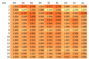
Figure 4: Performance effect of conjugating (c) and/or transposing (t) one or both sets of input single precision complex matrices with the baseline being no operation (n). Slower performance is indicated by darker colors and lower values (less than 1).

8.3 Improvement due to axpby_type template parameter

As mentioned earlier, the axpby_type template parameter can be used to reduce computation time for special values of $\alpha$ and $\beta$ while maintaining a general interface. Figure 5 shows the speed and performance gain for single precision matrices of sizes 1-16 when $\alpha=1$ and $\beta=0$. Depending on the matrix size, the gains are between 10% and 50% over the code that works for arbitrary $\alpha$ and $\beta$. Hence, the added complexity due to this extra template parameter is worth it.

Figure 5: Speed and performance gain for single precision matrices of various sizes when $\alpha=1$ and $\beta=0$ and for general values of these parameters.

8.4 Speed for various data types and matrix sizes

We now show the speeds achievable for four data types – real and complex types in single and double precision – for matrix sizes 1-16. We show results where $\alpha=1$ and $\beta=0$ in Figure 6. Naturally, using arbitrary $\alpha$ and $\beta$ will give a slightly lower performance than what is shown. For matrices of size 16 and $\alpha=1$ and $\beta=0$ on NVIDIA Tesla K20c, we reach these GFlop/s rates – 216 for single real, 173 for double real, 609 for single complex, and 217 for double complex. For general $\alpha$ and $\beta$, the speeds are lower by roughly 15%-30% for matrices of size 16.

Figure 6: Batched GEMM speed on NVIDIA Tesla K20c for various matrix sizes, various data types, and when $\alpha=1$ and $\beta=0$ (a1b0) or they are general values (ab).

8.5 Performance comparison with cuBLAS

We now compare cuBLAS and our two kernels – one which uses the second-order leading dimension and one using pointers to pointers just like cuBLAS batched interface.

As mentioned earlier, we have ignored memory allocation, deallocation, and transmission overhead required in cuBLAS for working with pointers to pointers. We have measured only the time spent in calling GEMM. Similarly, we have ignored timing these steps for out kernels, but naturally this time will be less than what is required in cuBLAS interface.

See Figure 7 for the real case and Figure 8 for the complex case. Both our kernels are noticeably faster than cuBLAS for matrix sizes under 16 except for a handful of cases. The second order leading dimension based kernel, which is the one we intend to use, is slower in just one case out of all by 5%.

The results show that part of the improvement is due to our implementation and part of it is due to the changes in interface. Figure 9 shows the relative improvement for various matrix sizes in the case of improved interface. It can be up to 600% for small sizes. Table 1 lists the speed we achieve when multiplying 100,000 independent matrix pairs of various sizes using the TGEMM_multi_uniform kernel on NVIDIA Tesla K20c.

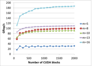
(a) Single precision real

(b) Double precision real

Figure 7: Comparison of the speed of our two kernels and cuBLAS batched implementation for real scalars and $\alpha=1$ and $\beta=0$. Relative improvement is shown in Figure 9.

(a) Single precision complex

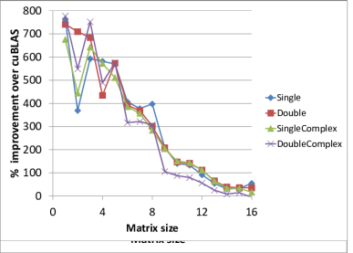
(b) Double precision complex

Figure 8: Comparison of the speed of our two kernels and cuBLAS batched implementation for complex scalars and $\alpha=1$ and $\beta=0$. Relative improvement is shown in Figure 9.

Size	Single-R	Double-R	Single-C	Double-C
1	1	1	2	2
2	3	4	10	9
3	12	11	42	34
4	26	17	87	52
5	48	39	143	102
6	59	48	187	100
7	83	68	263	146
8	125	86	327	204
9	102	86	334	127
10	104	90	362	149
11	126	110	439	172
12	129	122	480	186
13	124	114	446	172
14	126	115	436	177
15	150	131	504	212
16	216	173	609	217

Table 1: The GFlop/s rates when multiplying 100,000 independent matrix pairs of various sizes using the TGEMM_multi_uniform kernel on NVIDIA Tesla K20c. The comparison with corresponding numbers in cuBLAS are made in Figure 7 and Figure 8. The suffixes R and C stand for real and complex, respectively.

Figure 9: Relative improvement over cuBLAS batched implementation for various matrix sizes when our improved interface and implementation is used.

9 Discussion

We have described a new interface and two improved implementations of a batched GEMM routine. Another interesting batched GEMM case is when one matrix, either the one on the left or right, is fixed and one has to multiply it with a batch of other matrices. This can be treated by a non-batched GEMM implementation by concatenating matrices but high performance may not be readily possible because the non-batched GEMM might not be designed for such cases. However, based on our experience in this research, we believe that a special batched GEMM implementation for this case will be much faster than using non-batched GEMM. Naturally, it will be faster than our case where both matrices vary.

The second leading dimension based interface presented here can be extended to other BLAS routines naturally, for GPUs or multi-core CPUs. As of now, we don’t have data to quantify the importance of a batched GEMM implementation on GPU in high performance of other GPU-based BLAS routines for small matrices. However, just like the CPU case, we believe it will be crucial to formulate other batched BLAS kernels in terms of batched GEMM.

Acknowledgements

This work was partially supported by the US Department of Energy SBIR Grant DE-SC0004439.

References

- [1] R. Nath, S. Tomov, J. Dongarra, An Improved Magma Gemm For Fermi Graphics Processing Units, Int. J. High Perform. Comput. Appl. 24 (4) (2010) 511–515.
- [2] K. Goto, R. Van De Geijn, High-performance implementation of the level-3 blas, ACM Trans. Math. Softw. 35 (1) (2008) 4:1–4:14.
- [3] G. Karniadakis, S. Sherwin, Spectral/hp element methods for CFD, Oxford University Press, USA, 1999.
- [4] M. Deville, P. Fischer, E. Mund, High-Order Methods for Incompressible Fluid Flow, Cambridge University Press, 2002.
- [5] L. Demkowicz, Computing with hp-ADAPTIVE FINITE ELEMENTS: Volume I: One and Two Dimensional Elliptic and Maxwell Problems, Chapman & Hall/CRC Press, 2006.
- [6] L. Demkowicz, W. Rachowicz, D. Pardo, M. Paszynski, J. Kurtz, A. Zdunek, Computing with hp-ADAPTIVE FINITE ELEMENTS: Volume II Frontiers: Three Dimensional Elliptic and Maxwell Problems with Applications, Chapman & Hall/CRC Press, 2007.
- [7] P. Šolín, K. Segeth, I. Doležel, Higher-order Finite Element Methods, Chapman & Hall/CRC, 2003.
- [8] P. Bientinesi, V. Eijkhout, K. Kim, J. Kurtz, R. van de Geijn, Sparse direct factorizations through unassembled hyper-matrices, Computer Methods in Applied Mechanics and Engineering 199 (2010) 430–438.
- [9] B. Kågström, P. Ling, C. V. Loan, GEMM-based level 3 BLAS: high-performance model implementations and performance evaluation benchmark, ACM Transactions on Mathematical Software.
- [10] NVIDIA CUDA Basic Linear Algebra Subroutines (cuBLAS) library, https://developer.nvidia.com/cublas, accessed: Feb 21, 2013.
- [11] E. Anderson, Z. Bai, C. Bischof, S. Blackford, J. Demmel, J. Dongarra, J. Du Croz, A. Greenbaum, S. Hammarling, A. McKenney, D. Sorensen, LAPACK Users’ Guide, 3rd Edition, SIAM, Philadelphia, PA, 1999.
- [12] B. Stroustrup, The C++ Programming Language, 3rd Edition, Addison-Wesley Longman Publishing Co., Inc., Boston, MA, USA, 2000.
- [13] N. J. Higham, Stability of a method for multiplying complex matrices with three real matrix multiplications, SIAM J. Matrix Anal. Appl. 13 (3) (1992) 681–687.