Subspace-preserving sparsification of matrices with minimal perturbation to the near null-space. Part I: Basics

Abstract

This is the first of two papers to describe a matrix sparsification algorithm that takes a general real or complex matrix as input and produces a sparse output matrix of the same size. The non-zero entries in the output are chosen to minimize changes to the singular values and singular vectors corresponding to the near null-space of the input. The output matrix is constrained to preserve left and right null-spaces exactly. The sparsity pattern of the output matrix is automatically determined or can be given as input.

If the input matrix belongs to a common matrix subspace, we prove that the computed sparse matrix belongs to the same subspace. This works without imposing explicit constraints pertaining to the subspace. This property holds for the subspaces of Hermitian, complex-symmetric, Hamiltonian, circulant, centrosymmetric, and persymmetric matrices, and for each of the skew counterparts.

Applications of our method include computation of reusable sparse preconditioning matrices for reliable and efficient solution of high-order finite element systems. The second paper in this series [1] describes our open-source implementation, and presents further technical details.

1 Introduction

We present and analyze a matrix-valued optimization problem formulated to sparsify matrices while preserving the matrix null-spaces and certain special structural properties. Algorithms for sparsification of matrices have been used in various fields to reduce computational and/or data storage costs. Examples and applications are given in [2, 3, 4, 5] and the references therein. In general, these techniques lead to small perturbations only in the higher end of the spectrum and don’t respect the null-space or near null-space. This is intentional and not necessarily a limitation of these algorithms.

We have different objectives for sparsification. First, we want to preserve input matrix structural properties related to matrix subspaces, if it has any. Being Hermitian or complex-symmetric are just a couple of examples of such properties. Second, we want sparsification to minimally perturb the singular values and both left and right singular vectors in the lower end of the spectrum. Third, we want to exactly preserve the left and right null-spaces if there are any.

Our main contribution in this paper is designing an algorithm that fulfills all the three objectives mentioned above. We also provide theoretical results and numerical experiments to support our claims. The algorithm presented here is inspired from a less general but a similar sparsification algorithm introduced in our earlier publication [6]. That algorithm, in turn, was inspired from the results presented in [7]. Understanding the previous versions of the algorithm is not a prerequisite for understanding the one presented here.

There has been a related work where one solves an optimization problem to find a sparse preconditioner [8]. However, the function to be minimized there was non-quadratic and non-smooth, the method worked only for symmetric positive-definite matrices, the sparsity patterns were supposed to be chosen in advanced, and the method was quite slow. Our algorithm does not produce the optimal sparsified matrix as measured by condition number. Nonetheless, it does not suffer from these limitations and produces preconditioning matrices that are competitive in terms of condition number.

Our first objective, of maintaining structure, is important for aesthetic as well as practical reasons. If an algorithm produces an asymmetric matrix by sparsifying a symmetric matrix, it just doesn’t look like an “impartial” algorithm. On the practical side, if a property like symmetry were lost, one would have to resort to data structures and algorithms for asymmetric matrices which, in general, will be slower than those for symmetric matrices. The second and third objectives – not disturbing the near null-spaces and the corresponding singular values while also preserving the null-spaces – are important when the inverse of the matrix is to be applied to a vector rather than the matrix itself. Then, the inverse, or the pseudo-inverse, of the sparsified matrix can then be used in place of the inverse of the dense matrix without incurring a large error due to sparsification. This also means that the sparsified matrix can be used to compute a preconditioner with the likelihood that computation with it will be less expensive due to the sparsity we introduce.

To fulfill these objectives, we design and analyze a matrix-valued, linearly constrained convex quadratic optimization problem. It works for a general real or complex matrix, not necessarily square, and produces a sparse output matrix of the same size. A suitable pattern for sparsity is also computed. The user can control the sparsity level easily. We prove that the output sparse matrix automatically belongs to certain subspaces without imposing any constraints for them if the input matrix belongs to them. In particular, this property holds for Hermitian, complex-symmetric, Hamiltonian, circulant, centrosymmetric, and persymmetric matrices and also for each of the skew counterparts.

We briefly mention that the rows and columns of the input matrix should be well-scaled for the best performance of our sparsity pattern computation method. A rescaling by pre- and post-multiplication by a diagonal matrix leads to a well-scaled input matrix [9]. We intend to highlight the effects of scaling to our algorithm in a future publication.

In practice, we are concerned with matrices of size less than a few thousands. Applications of our method include computation of reusable sparse preconditioning matrices for reliable and efficient (in time consumed and memory used) techniques for solutions of high-order finite element systems, where the element stiffness matrices are the candidates for sparsification [6]. We want to stress that the sparsification process is somewhat expensive because we need to solve a matrix-valued problem and we want to respect the null-space and the near null-space rather than the other end of the spectrum. However, we can reuse the computed sparse matrices for multiple elements. We have also modified the algorithm slightly to speed it up by orders of magnitude and this is described in the next paper in the series [1].

Intuitively, any sparsification algorithm with objectives like ours will be more useful when a large fraction of the input matrix entries has small but non-zero magnitude relative to the larger entries. Typical high-order finite element matrices have this feature due to approximate cancellation that happens when high order polynomials are integrated in the bilinear form. On the other extreme, Hadamard matrices are poor candidates for sparsification like ours.

Of course, special techniques in some situations can generate sparse stiffness matrix without any explicit sparsification [10]. However, our objective is to be as general as possible and let the sparsification handle any kind of input matrix.

The second paper [1] describes version 1.0 of TxSSA, which is a library implemented in C++ and C with interfaces in C++, C, and MATLAB. It is an implementation of our sparsification algorithm. TxSSA is an acronym for Tech-X Corporation Sparse Spectral Approximation. The code is distributed under the BSD 3-clause open-source license and is available here.

http://code.google.com/p/txssa/

Here is an outline of the paper. In Section 2, we describe the optimization problem, provide a rationale for the choices we make, and prove that it is well-posed. In Section 3, we describe the algorithm for computing the sparsity pattern and state some of its properties. In Section 4, we prove a few theoretical bounds that relate the output matrix to the input matrix and other input parameters. In Section 5, we prove that our algorithm preserves many important matrix subspaces. Finally, in Section 6, we show some basic numerical results. Detailed results and other practical concerns are given in the second paper of this series [1].

2 An optimization problem for sparsification

We work with rectangular complex matrices and complex vectors. Simplifications to the real or square case are straightforward.

2.1 Notation

Let $\mathbb{\mathbb{C}}^{m\times n}$ denote the vector space of rectangular complex matrices with $m$ rows and $n$ columns. Let $\mathbb{\mathbb{C}}^{m}$ denote the vector space of complex vectors of size $m$. The superscripts ‘T’, ‘*’, and ‘$\dagger$’ denote transpose, conjugate transpose, and the Moore-Penrose pseudoinverse respectively. A bar on top of a quantity implies complex conjugate. Let $\mathcal{N}(\cdot)$ denote the null-space and $\mathcal{R}(\cdot)$ denote the range-space of a matrix. The default norm used for matrices is the Frobenius norm. For vectors the Euclidean norm is the default. Otherwise norms have specific subscripts. As usual, the identity matrix of size $n$ is denoted by $I_{n}$. The symbol $I$ is used in case the size is easily deducible.

Let $A\in\mathbb{\mathbb{C}}^{m\times n}$ be the input matrix to be sparsified. The matrix $A$ can be expressed using the singular value decomposition (SVD) as $U\Sigma V^{*}$. Let $r:=\text{rank}(A)$. The singular values of $A$ are $\left\{{\sigma}_{i}\right\}_{i=1}^{\min(m,n)}$ sorted in non-increasing order, the right singular vectors are $\left\{{v}_{i}\right\}_{i=1}^{n}$, and the left singular vectors are $\left\{{u}_{i}\right\}_{i=1}^{m}$. We divide $U$ and $V$ into two blocks each based on the rank $r$. We get

$$A=U\Sigma V^{*}=\left[U_{1}\;U_{2}\right]\Sigma\left[V_{1}\;V_{2}\right]^{*}$$

where $U_{1}$ and $V_{1}$ each have $r$ columns. Similarly,

$$\Sigma=\begin{bmatrix}\Sigma_{r}&0\\ 0&0\\ \end{bmatrix}$$

where $\Sigma_{r}$ is of size $r\times r$, diagonal, and invertible unless $r=0$. The columns in $U_{1}$ and $V_{1}$ form orthonormal basis for $\mathcal{R}(A)$ and $\mathcal{R}(A^{*})$, respectively. Similarly, the columns in $U_{2}$ and $V_{2}$ form orthonormal basis for $\mathcal{N}(A^{*})$ and $\mathcal{N}(A)$, respectively.

Using the rank-nullity theorem, we get

$$p_{R}:=\text{dim}(\mathcal{N}(A))=n-r$$

where $p_{R}$ is the “right nullity”. Similarly,

$$p_{L}:=\text{dim}(\mathcal{N}(A^{*}))=m-r$$

where $p_{L}$ is the “left nullity”. Thus, $\mathcal{N}(A^{*})\in\mathbb{\mathbb{C}}^{m\times p_{L}}$ and $\mathcal{N}(A)\in\mathbb{\mathbb{C}}^{n\times p_{R}}$.

Let $\kappa=\kappa(A):=\left|\left|A\right|\right|_{2}\left|\left|{A}^{\dagger}\right|\right|_{2}$ be a condition number for rank-deficient matrices. Obviously, $\kappa=\frac{\sigma_{1}(A)}{\sigma_{r}(A)}\geq 1$ for non-zero matrices and it generalizes the usual condition number, which is typically used for square non-singular matrices.

Let $\mathcal{Z}=\mathcal{Z}(A)\in\mathbb{\mathbb{R}}^{m\times n}$ be a matrix that denotes a sparsity pattern corresponding to $A$. It contains zeros and ones only. A zero in $\mathcal{Z}$ means the entry at the corresponding position in the output matrix is fixed to be zero. A one in $\mathcal{Z}$ means the entry at corresponding position will be allowed to vary and can be non-zero. The pattern matrix is always real even for complex input matrices. We do not create separate patterns for real and imaginary parts of a complex matrix. The rationale behind this choice will be explained later in Remark 3.10 in Section 3.4, where we will also provide a concrete algorithm for computing $\mathcal{Z}(A)$ .

2.2 A misfit functional

Let $X=X(A)\in\mathbb{\mathbb{C}}^{m\times n}$ be a matrix produced by sparsification of $A$. Fix $X_{ij}=0$ if $\mathcal{Z}_{ij}=0$. When the sparsity pattern is fixed, $X$ belongs to a subspace of $\mathbb{\mathbb{C}}^{m\times n}.$ Here, $i$ and $j$ are indices such that $1\leq i\leq m$ and $1\leq j\leq n$.

We define an SVD based quadratic “misfit” functional $J\in\mathbb{R}$ to specify a difference between input matrix $A$ and an arbitrary matrix $X$.

Definition 2.1.

$$J=J(X;A):=\frac{1}{2}\sum_{i=1}^{r}\frac{1}{\sigma_{i}^{2}}\left|\left|(X-A)v_{i}\right|\right|^{2}_{2}+\frac{1}{2}\sum_{i=1}^{r}\frac{1}{\sigma_{i}^{2}}\left|\left|(X^{*}-A^{*})u_{i}\right|\right|^{2}_{2}$$ (1)

This misfit quantifies the action of the unknown matrix $X$ on the singular vectors of $A$ and penalizes the differences in near null-space with larger “weights”. This is just a symbolic expression for defining $J$. We shall see in Section 2.4 that the SVD of $A$ does not have to be computed to compute $J$ and its derivatives.

We now pose a linearly constrained quadratic optimization problem to compute $X$.

$$\min_{X}J(X;A)$$ such that

$$\mathcal{N}(A)\subseteq\mathcal{N}(X),$$

$$\mathcal{N}(A^{*})\subseteq\mathcal{N}(X^{*}),\text{ and }$$

$$X\text{ has a specified sparsity pattern }\mathcal{Z}(A)$$ (2)

It is readily seen that the constraints are linear homogeneous equality constraints and $J$ is a quadratic function in the entries of $X$. Additionally, the misfit $J(X;A)$ is quadratic and bounded below by zero for any $X$ whether the constraints are imposed or not. This is one way to see that it is also a convex function of $X$. We can rewrite the minimization problem as follows.

$$\min_{X}J(X;A)\text{ such that }XV_{2}=0,X^{*}U_{2}=0,\text{ and }X_{ij}=0\text{ if }(\mathcal{Z}(A))_{ij}=0.$$ (3)

2.3 Rationale for the two-term misfit

We had posed a similar minimization problem in [6]. We used it to construct sparse preconditioners for high-order finite element problems. However, the input matrix $A$ had to be real and symmetric. The output matrix was specifically constrained to be symmetric. The misfit there had only one term, rather than two as shown here, because symmetry of $A$ and $X$ implied that the two terms were equal and hence one was redundant. For the same reason only the right null-space was imposed. The left null-space constraint, or equivalently, the constraint related to the conjugate-transpose matrix’s null-space, became redundant. Generalization to asymmetric matrices is one of the contributions of the current research.

We now work with an arbitrary input matrix (complex, rectangular) and thus make the setting completely general. This is done by working with the singular values and singular vectors rather than eigenvalues and eigenvectors. We have also avoided explicit imposition of structural constraints, like matrix symmetry.

There are multiple reasons behind the choice of not using explicit structural constraints. In many cases, it is indeed possible to impose linear equality constraints to impose that $X$ belong to a certain subspace of matrices. However, explicit specification would lead to specialized code for any new subspace. For example, special handling of Hermitian, complex-symmetric, Hamiltonian, and many other matrices would be needed. Although imposing such constraints individually is simple, explicitly imposing such constraints doesn’t tell us what to do in case of matrices without common structures. Consider a general matrix $A$ such that $\left|\left|A-A^{*}\right|\right|\approx 0.001\left|\left|A\right|\right|$. It is reasonable to expect and desire a similar small difference in $X$ and $X^{*}$. However, in general, we cannot impose an affine equality constraint to impose this. Thus, even a tiny perturbation in input that destroys some structure results in a completely different mathematical and computational problem (assuming we were actually explicitly imposing $X=X^{*}$ when $A=A^{*}$). These considerations motivated us to design a new algorithm where no such constraints are needed. We now use a two-term misfit, two null-space related constraint sets, and abandon such explicit constraints even in cases where it is meaningful. We show in Section 5 that such an algorithm still preserves matrix structural properties whenever they are present.

2.4 Avoiding the SVD

We now show that the misfit in Equation (1) can be expressed in terms of the Moore-Penrose pseudoinverse of the input matrix $A$. This avoids using its singular values and singular vectors for actual computation. We expressed the misfit using SVD first to show that the misfit penalizes deviations in the lower end of the spectrum of $A$ and to motivate the formulation. See Section 2.1 for the notation.

Lemma 2.2.

Let $A,Y\in\mathbb{\mathbb{C}}^{m\times n}$. Let $A=U\Sigma V^{*}$ be its SVD. Then

$$\sum_{i=1}^{r}\frac{1}{\sigma_{i}^{2}}\left|\left|Yv_{i}\right|\right|^{2} =\left|\left|Y{A}^{\dagger}\right|\right|^{2},\text{ and}$$

$$\sum_{i=1}^{r}\frac{1}{\sigma_{i}^{2}}\left|\left|Y^{*}u_{i}\right|\right|^{2} =\left|\left|Y^{*}{(A^{*})}^{\dagger}\right|\right|^{2}.$$

Proof.

Using the SVD based expression for the Moore-Penrose pseudoinverse and the fact that the Frobenius matrix norm is invariant under multiplication by a unitary matrix, it is easily seen that

$$\left|\left|Y{A}^{\dagger}\right|\right|^{2}=\left|\left|YV{\Sigma}^{\dagger}U^{*}\right|\right|^{2}=\left|\left|YV{\Sigma}^{\dagger}\right|\right|^{2}.$$

The last term can be expanded to a summation using $v_{i}$, the columns of $V$, and $\frac{1}{\sigma_{i}}$, the non-zero diagonal values of ${\Sigma}^{\dagger}$. This results in the left hand side of the first equality. Thus the first equality holds. The second equality can be derived in the same fashion. ∎

The previous result and the property that $\left|\left|Y\right|\right|=\left|\left|Y^{*}\right|\right|$ are used to express the misfit $J$ from Equation (1) as

$$J(X;A)=\frac{1}{2}\left|\left|(X-A){A}^{\dagger}\right|\right|^{2}_{F}+\frac{1}{2}\left|\left|{A}^{\dagger}(X-A)\right|\right|^{2}_{F}$$ (4)

This avoids the use of singular vectors and singular values and one avoid using the SVD. The pseudoinverse or a reasonable approximation to it can be computed by any algorithm that is suitable depending on the conditioning and any known matrix properties. By way of example, if the rank-revealing QR algorithm reliably determines the numerical rank of $A$, it can be used to compute an accurate pseudoinverse. On the other hand if $A$ were symmetric semi-definite too, the pivoted Cholesky will be faster for computing the pseudoinverse.

This is a good place to mention that we are indeed making the assumption that the condition number of the input matrix is not “too large”. This assumption is made so that one can avoid SVD and use a faster but less robust algorithm to compute the pseudoinverse. More importantly, if the condition number of $A$ were very large, its invariant spaces will be highly sensitive to any perturbation applied to $A$. Sparsifying might be worthless even if SVD is used. What is a “too large” condition number can can be quantified after some numerical experimentation and will also strongly depend on the relative number of zeros introduced via sparsification.

2.5 First-order optimality conditions

We derive the first-order optimality conditions for the minimization problem using the method of Lagrange multipliers. Since the quadratic form in Equation (2.2) is convex for all $A$ (see Section 2.2) and the set of feasible points is convex, any stationary point will be a local minima. Hence it is sufficient to consider solutions of the first-order optimality conditions.

2.5.1 The Lagrange multipliers

We introduce the Lagrange function $\mathcal{L}=\mathcal{L}(X,\Lambda_{R},\Lambda_{L},\Lambda_{\mathcal{Z}};A)$, where $X$ is the unknown sparse matrix, $\Lambda_{R}\in\mathbb{\mathbb{C}}^{m\times p_{R}}$ and $\Lambda_{L}\in\mathbb{\mathbb{C}}^{n\times p_{L}}$ are matrices of Lagrange multipliers corresponding to the right and left null-space constraints, respectively. To impose the sparsity pattern, we use a matrix $\Lambda_{\mathcal{Z}}\in\mathbb{\mathbb{C}}^{m\times n}$, a matrix of Lagrange multipliers and zeros. If $(\mathcal{Z}(A))_{ij}=0$, $(\Lambda_{\mathcal{Z}})_{ij}=\mu_{ij}\in\mathbb{C}$ else $(\Lambda_{\mathcal{Z}})_{ij}=0$.

$$\mathcal{L}(X,\Lambda_{R},\Lambda_{L},\Lambda_{\mathcal{Z}};A):= \frac{1}{2}\left|\left|(X-A){A}^{\dagger}\right|\right|^{2}+\frac{1}{2}\left|\left|{A}^{\dagger}(X-A)\right|\right|^{2}$$

$$+ \;\text{trace}(\Lambda_{R}^{*}XV_{2})$$

$$+ \;\text{trace}(\Lambda_{L}^{*}X^{*}U_{2})$$

$$+ \;\sum_{\begin{subarray}{c}ij\text{ where }\\ (\mathcal{Z}(A))_{ij}=0\end{subarray}}\mu_{ij}X_{ij}$$

2.5.2 Derivative of the misfit

Before differentiating $\mathcal{L}$, we write the derivative of $J$ with respect to $X$. We get

$$\frac{\partial J}{\partial X} =(X-A){A}^{\dagger}({A}^{\dagger})^{*}+({A}^{\dagger})^{*}{A}^{\dagger}(X-A)$$

$$=\left(X{A}^{\dagger}({A}^{\dagger})^{*}+({A}^{\dagger})^{*}{A}^{\dagger}X\right)-\left(A{A}^{\dagger}({A}^{\dagger})^{*}+({A}^{\dagger})^{*}{A}^{\dagger}A\right)$$

$$=\left(X{A}^{\dagger}({A}^{\dagger})^{*}+({A}^{\dagger})^{*}{A}^{\dagger}X\right)-2({A}^{\dagger})^{*}$$

The simplification done above, in the terms not involving $X$, can be proved easily using the SVD based expression of the Moore-Penrose pseudoinverse.

Using the relation between the “vectorization operation” and the Kronecker product, we get

$$\text{vec}\left(\frac{\partial J}{\partial X}\right)=\left({A}^{\dagger}({A}^{\dagger})^{*}\otimes I_{m}+I_{n}\otimes({A}^{\dagger})^{*}{A}^{\dagger}\right)\text{vec}(X)$$

where $I_{k}$ is the identity matrix of size $k$. We define the $mn\times mn$ Kronecker sum matrix $\mathcal{A}=\mathcal{A}(A)$ as

$$\mathcal{A}=\mathcal{A}(A):={A}^{\dagger}({A}^{\dagger})^{*}\otimes I_{m}+I_{n}\otimes({A}^{\dagger})^{*}{A}^{\dagger}$$ (5)

Using the spectral properties of Kronecker sums, it is obvious that $\mathcal{A}(A)$ is always Hermitian positive semi-definite. It is Hermitian positive definite if and only if $A$ is full-rank. We skip the proofs.

2.5.3 Derivative of the Lagrangian

We differentiate the Lagrangian given in Section 2.5.1 to derive the first order optimality conditions. Instead of presenting the intermediate steps in the derivation we write the final expressions only. Appendix A in [11] shows the intermediate steps for matrix-valued derivatives.

$$\frac{\partial\mathcal{L}}{\partial X}=0\implies X{A}^{\dagger}({A}^{\dagger})^{*}+({A}^{\dagger})^{*}{A}^{\dagger}X+\Lambda_{R}V_{2}^{*}+U_{2}\Lambda_{L}^{*}+\Lambda_{\mathcal{Z}}=2({A}^{\dagger})^{*}$$

$$\frac{\partial\mathcal{L}}{\partial\Lambda_{R}}=0\implies XV_{2}=0$$

$$\frac{\partial\mathcal{L}}{\partial\Lambda_{L}}=0\implies X^{*}U_{2}=0$$

$$\frac{\partial\mathcal{L}}{\partial\mu_{ij}}=0\implies X_{ij}=0\text{ for }ij\text{ such that }(\mathcal{Z}(A))_{ij}=0$$

2.6 Existence and global uniqueness of the minimizer

We show that the minimization problem posed in Equation (2.2) and with the linear system shown in Section 2.5.3 has a unique solution for any input matrix $A$ and any imposed sparsity pattern. This is true even if the sparsity pattern has no relation to the input matrix $A$.

Lemma 2.3.

A minimizer always exists for the minimization problem posed in Equation (2.2) for an arbitrary imposed sparsity pattern.

Proof.

The equality constraints for null-spaces and sparsity are linear and homogeneous. Thus, the set of feasible solutions is non-empty. For example, the zero matrix is a feasible element. Since the quadratic form is convex for all $X$ (see Section 2.2), a minimizer always exists [12]. ∎

We now have to prove that there is a globally unique minimizer. We do this first for the full-rank $A$ and then for a non-zero rank-deficient $A$.

Lemma 2.4.

If $A$ is full-rank, the minimization problem posed in Equation (2.2) has a globally unique minimizer for an arbitrary imposed sparsity pattern.

Proof.

As mentioned in Section 2.5.2, the quadratic form $J$ is strictly convex on $\mathbb{\mathbb{C}}^{m\times n}$ if $A$ is full-rank. In particular, it is strictly convex on the subspace of those matrices that satisfy the equality constraints. Since the feasible set is convex and non-empty, the minimizer is globally unique. ∎

Lemma 2.5.

If $A$ is non-zero and rank-deficient, the minimization problem posed in Equation (2.2) has a globally unique minimizer for an arbitrary imposed sparsity pattern.

Proof.

For rank-deficient matrices the Hessian of the quadratic form is merely positive semi-definite on $\mathbb{\mathbb{C}}^{m\times n}$. But we show that it is positive definite on the subspace of matrices that satisfy the null-space related constraints. Showing this will ensure that the Hessian is positive definite on the subspace of matrices satisfying all the constraints (which includes sparsity constraints also). This, in turn, means that there is a globally unique minimizer even for the rank-deficient case.

Using the fact that $U$ and $V$ are unitary, it can be easily shown that all matrices $X$ that satisfy the null-space constraints can be written as a linear combination of $r^{2}$ basis matrices using arbitrary complex coefficients $\left\{\alpha_{ij}\right\}_{i,j=1}^{r}$.

$$X=\sum_{i=1}^{r}\sum_{j=1}^{r}\alpha_{ij}\;u_{i}v_{j}^{*}$$

As defined earlier, $u_{i}$ and $v_{j}$ are the left and right singular vectors of $A$ respectively.

Consider the action of the Kronecker sum matrix $\mathcal{A}(A)$ (Equation (5)) on the vectorized basis matrices $u_{i}v_{j}^{*}$.

$$\mathcal{A}(A)\text{vec}(u_{i}v_{j}^{*}) =\left({A}^{\dagger}({A}^{\dagger})^{*}\otimes I_{m}+I_{n}\otimes({A}^{\dagger})^{*}{A}^{\dagger}\right)\text{vec}(u_{i}v_{j}^{*})$$

$$=\text{vec}\left(u_{i}v_{j}^{*}{A}^{\dagger}({A}^{\dagger})^{*}+({A}^{\dagger})^{*}{A}^{\dagger}u_{i}v_{j}^{*}\right)$$

$$=\text{vec}\left(u_{i}\frac{u_{j}^{*}}{\sigma_{j}}({A}^{\dagger})^{*}+({A}^{\dagger})^{*}\frac{v_{i}}{\sigma_{i}}v_{j}^{*}\right)$$

$$=\text{vec}\left(u_{i}\frac{1}{\sigma_{j}^{2}}v_{j}^{*}+u_{i}\frac{1}{\sigma_{i}^{2}}v_{j}^{*}\right)$$

$$=\left(\frac{1}{\sigma_{i}^{2}}+\frac{1}{\sigma_{j}^{2}}\right)\text{vec}(u_{i}v_{j}^{*})$$

Since both $i,j\leq r$, $\sigma_{i}>0$ and $\sigma_{j}>0$. Thus, $\text{vec}(u_{i}v_{j}^{*})$ are eigenvectors of the Hessian matrix and the corresponding eigenvalues are positive. Hence, the Hessian restricted to the subspace of matrices that satisfy the null-space constraints is positive definite. ∎

Theorem 2.6.

A globally unique minimizer exists for the minimization problem posed in Equation (2.2) for an arbitrary imposed sparsity pattern.

Proof.

This is a consequence of the three lemmas proved earlier $-$ Lemmas 2.3, 2.4, 2.5, and the easily seen fact that if $A=0$, then $X=0$ is the only feasible solution. ∎

3 An $L_{p}$ norm based algorithm to compute the sparsity pattern

In this section, we describe an algorithm for determination of sparsity pattern in detail, analyze its computational complexity, state and prove some of its properties, and provide the rationale behind a few subtle technical issues.

3.1 Overview of the sparsity pattern algorithm

We showed in Section 2.6 that the minimization problem to compute a sparse $X$ has a unique solution for any imposed sparsity pattern. However, the sparsity determination phase is separate than the minimization phase and it is important to have a well-defined and universal method of choosing a sparsity pattern rather than imposing something arbitrary.

We had presented an $L_{1}$ norm based algorithm designed for real square matrices in [6]. Here we generalize for arbitrary matrices while also using the $L_{p}$ norm.

As before, we also provide a single parameter $q$, continuously variable in the interval $[0,1]$, that allows a user to choose anywhere between the two extremes of very sparse ($q=0$) and no extra sparsity ($q=1$). Using a larger $q$ will provide a better approximation but will be more dense, whereas a smaller $q$ will provide a worse approximation but lead to fewer non-zeros in $X$.

In any case, we eliminate only those entries that are small in magnitude relative to other larger entries. Intuitively, this makes sense because eliminating small matrix entries will perturb the matrix and its spectrum relatively less.

In choosing entries with large magnitude, our algorithm compares entries in the same row and column rather than with all other matrix entries. This choice helps in obtaining many important properties of the algorithm. The details and rationale are provided later in Section 3.5.

3.2 Definition of an $L_{p}$ norm based sparsity for vectors

Before describing the sparsity pattern algorithm for a matrix, we describe it for a single vector $x\in\mathbb{\mathbb{C}}^{m}$. This will be the key ingredient for the algorithm acting on a matrix.

Definition 3.1.

For any $p\in[0,\infty]$, we define the $L_{p}$ “norm” $\left|\left|x\right|\right|_{p}$ for any vector $x$.

$$\left|\left|x\right|\right|_{p}=\left\{\begin{array}[]{lcl}\displaystyle\left(\sum_{i=1}^{m}\left|x_{i}\right|^{p}\right)^{\frac{1}{p}}&:&1\leq p<\infty\\ \displaystyle\max_{i}\left|x_{i}\right|&:&p=\infty\\ \displaystyle\sum_{i=1}^{m}\left|x_{i}\right|^{p}&:&0<p<1\\ \displaystyle\text{number of non-zero }x_{i}&:&p=0\end{array}\right.$$

Note that $\left|\left|x\right|\right|_{p}$ is a “norm” only when $p\in[1,\infty]$. It is not a “norm” for $p<1$. We simplify the notation and call it a norm always.

We want to compute a sparsity pattern $\mathcal{Z}(x)$ for $x\in\mathbb{\mathbb{C}}^{m}$. $\mathcal{Z}(x)\in\mathbb{\mathbb{R}}^{m}$. It contains zeros and ones only. A zero in $\mathcal{Z}$ means the entry at the corresponding position is fixed to be zero otherwise it is free to be modified.

3.2.1 A combinatorial minimization problem for vector sparsity pattern

We state below a combinatorial minimization problem for computing $\mathcal{Z}(x)$ so that the number of eliminated entries is maximized while the $L_{p}$ norm of the eliminated entries is bounded from above. It is a combinatorial optimization problem because we can place ones and zeros in $\mathcal{Z}(x)$ at arbitrary locations. In addition, the number of non-zeros in $\mathcal{Z}(x)$ is unknown a priori.

We specify the input parameters – $p\in[0,\infty]$, $q\in[0,1]$, and $N\in[0,\left|\left|x\right|\right|_{0}]$. Here $N$ refers to the minimum number of non-zeros to be preserved. It makes sense to have the upper limit for $N$ not greater than $\left|\left|x\right|\right|_{0}$, which is the number of non-zeros present in $x$. The necessity of $N$ will be discussed in Section 3.4.2. The symbol ‘$\circ$’ denotes entry-wise product of two entities.

Given $x,p,q,$ and $N$, compute $\mathcal{Z}(x)$ using

$$\begin{array}[]{l}\displaystyle\max_{\mathcal{Z}(x)}\left|\left|x-x\circ\mathcal{Z}(x)\right|\right|_{0}\text{ such that }\\ \displaystyle\qquad(\mathcal{Z}(x))_{i}=0\text{ or }1,\\[5.0pt] \displaystyle\qquad\left|\left|\mathcal{Z}(x)\right|\right|_{0}\geq N,\text{ and }\\[5.0pt] \displaystyle\qquad\left|\left|x-x\circ\mathcal{Z}(x)\right|\right|_{p}\leq(1-q)\left|\left|x\right|\right|_{p}\end{array}$$ (6)

If $x=0$, we define $\mathcal{Z}(x)=0\in\mathbb{\mathbb{R}}^{m}$.

Before presenting an algorithm for computing $\mathcal{Z}(x)$, we remark on a few subtle cases.

Remark 3.2.

We allow $q$ to take the extreme values, zero or one, in the definition, but in practical cases it will take an intermediate value usually in $[0.5,1)$.

The form of the $q$ related inequality condition in our problem is motivated by two reasons $-$ maintaining a role for $q$ in $p=\infty$ case and better discrimination power for large $p$ case. We explain this in the remarks below.

Remark 3.3.

One reason we define the $q$ related inequality in terms of $L_{p}$ norm of eliminated entries $(\left|\left|x-x\circ\mathcal{Z}(x)\right|\right|_{p})$ and not in terms of the norm of preserved entries $(\left|\left|x\circ\mathcal{Z}(x)\right|\right|_{p})$ has to do with the large $p$ case, especially $p=\infty$. Assume $p=\infty$ and $q<1$ and we impose $\left|\left|x\circ\mathcal{Z}(x)\right|\right|_{p}\geq q\left|\left|x\right|\right|_{p}$ instead. In this case, preserving the entry (or entries) with the maximum magnitude would mean that the norm of preserved entries $\left|\left|x\circ\mathcal{Z}(x)\right|\right|_{p}$ is greater than $q\left|\left|x\right|\right|_{p}$. Since this is true for any $q<1$, that parameter becomes useless. This is avoided in Equation (6) by choosing a different inequality.

Remark 3.4.

Another reason for using the norm of eliminated entries is when $p$ is large but not necessarily infinite. In such a case, moving the smallest entry in the preserved part to eliminated part will affect the norm of eliminated part much more. Thus, comparing the norm of eliminated part with total norm has more “discrimination power”, specially for large $p$. For small $p$, close to one or even less than it, norms of both parts $-$ eliminated and preserved $-$ are affected roughly equally by such a move.

3.3 An algorithm to compute sparsity for vectors

We now present an algorithm to compute the sparsity pattern $\mathcal{Z}(x)$ for the problem posed in Equation (6). See Algorithm 1.

Data: $x\in\mathbb{\mathbb{C}}^{m},p\in[0,\infty],q\in[0,1],$ and $N\in[0,\left|\left|x\right|\right|_{0}]$

Result: Sparsity pattern $\mathcal{Z}(x)\in\mathbb{\mathbb{R}}^{m}$ with $(\mathcal{Z}(x))_{i}=$ 0 or 1

$(\mathcal{Z}(x))_{i}\leftarrow 0$ for $i=1,\ldots,m$;

$j\leftarrow num\_zeros(x)$;

if $j=m$ then

       return;

      

end if

$x$ $\leftarrow\mbox{abs}(x)$;

$ids\leftarrow[1,2,\ldots,m]$;

Sort $(x,ids)$ pairs in an ascending order with $x_{i}$ values as the keys;

// Eliminate entries until a threshold is not crossed

while $j<m-N$ do

       if $\left|\left|x(1:j+1)\right|\right|_{p}>(1-q)\left|\left|x\right|\right|_{p}$ then

             break;

            

      else

             $id\leftarrow ids(j)$;

             $(\mathcal{Z}(x))_{id}\leftarrow 1$;

             $j\leftarrow j+1$;

            

       end if

      

end while

// Preserve the remaining entries

while $j\leq m$ do

       $id\leftarrow ids(j)$;

       $(\mathcal{Z}(x))_{id}\leftarrow 1$;

       $j\leftarrow j+1$;

      

end while

Algorithm 1 An algorithm to compute sparsity pattern of a given real or complex vector. See Equation (6) for details.

Remark 3.5.

If there are multiple candidate entries in $x$ with the same magnitude that can lead to a non-unique $\mathcal{Z}(x)$, then any one of them can be used. This is a “corner case” and a simple rule like using all the equal values, even if fewer than all are sufficient, will break the tie and give a deterministic algorithm. In practical problems, we don’t expect that the vector will have a huge number of equal and large entries of exactly equal magnitude.

Theorem 3.6.

Algorithm 1 solves the optimization problem posed in Equation (6) to find the sparsity pattern for a given vector.

Proof.

We start with the three constraints in Equation (6). Obviously, the output $\mathcal{Z}(x)$ is such that $(\mathcal{Z}(x))_{i}=0\text{ or }1$. The second “while” loop ensures that $\left|\left|\mathcal{Z}(x)\right|\right|_{0}\geq N$. The first while loop makes sure that $\left|\left|x-x\circ\mathcal{Z}(x)\right|\right|_{p}\leq(1-q)\left|\left|x\right|\right|_{p}$ and the second one can only decrease $\left|\left|x-x\circ\mathcal{Z}(x)\right|\right|_{p}$.

Hence all the conditions are maintained and the issue is whether the output pattern maximizes the number of eliminated entries. It is clear from the algorithm that if a particular entry is eliminated, all entries smaller than that must have been eliminated. Assume that we want to eliminate one more (non-zero) entry. Doing this will violate the either the second or the third constraint in Equation (6) depending on which of the two was the active one in limiting the number of ones in $\mathcal{Z}(x)$. ∎

3.3.1 Computational complexity for sparsity pattern of vectors

For a vector of size $m$, Algorithm 1 runs in $O(m\log(m))$ operations. This assumes that an $O(m\log(m))$ algorithm is used for sorting. Hence the overall complexity is $O(m\log(m))$.

3.4 Definition of an $L_{p}$ norm based sparsity for matrices

We use the sparsity pattern computation algorithm for vectors described in Section 3.3 to compute a sparsity pattern for matrices. The algorithm for matrices can be divided into three separate steps. The first two steps can be executed independently and thus in any order. Assume we have a matrix $A\in\mathbb{\mathbb{C}}^{m\times n}$, and parameters $p$, $q$. We also need the parameters $N_{row}$ and $N_{col}$, which are used to specify minimum number of non-zeros in each row and each column, respectively. In Section 3.4.2 we will see how $N_{row}$ and $N_{col}$ are determined and specified a natural way. Here are the three steps for computing $\mathcal{Z}(A)$.

1. Compute the pattern in each of the $m$ separate rows (treated as vectors).

2. Compute the pattern in each of the $n$ separate columns (treated as vectors).

3. The final pattern $\mathcal{Z}(A)$ is the union, a boolean OR, of the row-based pattern and the transpose of column-based pattern.

The algorithm presented above is a specific choice that satisfies many useful theoretical properties. See Section 3.5.

Remark 3.7.

If it is known that the entry-wise absolute value matrix is symmetric, then we compute either the row or column pattern and take the union with its transpose. This shortcut is not necessary but is faster. Moreover, whether one takes the shortcut or not, the result is that the pattern is symmetric for matrices that are Hermitian, skew-Hermitian, or complex-symmetric.

Remark 3.8.

In general, the number of non-zeros will vary in each row and column depending on the distribution of the magnitudes of the entries. In this sense, this is an adaptive method and one does not know the number of non-zeros a priori for a given set of parameters.

Remark 3.9.

The algorithm works naturally with rectangular and complex matrices.

Remark 3.10.

We compute a single pattern matrix for complex matrices rather than separate independent patterns matrices for real and imaginary parts for two distinct reasons $-$ one theoretical and one practical. Firstly, when a single pattern is computed, the pattern remains invariant if the input matrix is multiplied by a non-zero complex number (see Property 2 in Section 3.5). This property will not hold in general when two patterns are computed. Secondly, storing two patterns for the sparsified $X$, for the real and imaginary parts, increases the storage costs and one cannot use complex arithmetic for first-order optimality conditions (see Section 2.5.3).

3.4.1 Computational complexity for sparsity pattern of matrices

We discuss the computational complexity for each of the three steps in Section 3.4 using the computational complexity for sparsity pattern of vectors in Section 3.3.1.

1. Computing the sparsity pattern for $m$ rows requires $m(n\log(n))$ operations in total.

2. Computing the sparsity pattern for $n$ columns requires $n(m\log(m))$ operations in total.

3. Computing the union operation is relatively more complex. Creating the transpose of a sparse matrix takes $O(mn)$ operations. After transposing, the union is computed row by row. Computing union of the patterns of two row vectors of size $n$ each takes $O(n\log(n))$ operations. This is done $m$ times.

Hence, the overall cost is still $O(mn(\log(m)+\log(n)))$ which can be expressed as $O(mn\log(mn))$.

3.4.2 Interaction of sparsity and null-space

We mentioned earlier that we can specify the parameters $N_{row}$ and $N_{col}$ when computing the sparsity pattern of a matrix. The two values are used to specify minimum number of non-zeros in each row and each column, respectively. Here we show why one needs these parameters.

Consider a matrix $X\in\mathbb{\mathbb{C}}^{m\times n}$ with a given sparsity pattern $\mathcal{Z}(A)$. When solving the optimization problem posed in Section 2.2, the unknown entries in each row of $X$ have to satisfy $p_{R}$ linear homogeneous equality constraints (see Section 2.1). If the number of allowed non-zero entries in a row of $\mathcal{Z}(A)$ is less than or equal to $p_{R}=\text{dim}(\mathcal{N}(A))$, then all the entries must be zero, and thus the whole row is zero. This is an undesirable situation. The same logic applies to columns and left null-space. Thus, an algorithm that decides the sparsity pattern should also keep sufficient number of non-zeros in each row and each column so that such degenerate matrix is not produced. In practice, we choose $N_{row}=\min(n,p_{R}+1)$ and $N_{col}=\min(m,p_{L}+1)$.

This restriction implies that the null-space dimension must be known before computing the sparsity pattern. Another implication is that sparsification while maintaining null-space constraints cannot be very useful if a matrix is highly rank-deficient. In many applications the rank-deficiency is a small constant independent of matrix size and this is not a huge concern.

3.5 Properties of the $L_{p}$ norm based matrix sparsity patterns

We enumerate a few important properties of the sparsity patterns generated by the $L_{p}$ norm based algorithm of Section 3.4. Let $A\in\mathbb{\mathbb{C}}^{m\times n}$, and $\mathcal{Z}(A)\in\mathbb{\mathbb{R}}^{m\times n}$ denote its sparsity pattern matrix. The number of non-zero entries in $\mathcal{Z}(A)$ is expressed as $\left|\mathcal{Z}(A)\right|$. When we want to discuss a specific parameters $p$ and $q$, we write $\mathcal{Z}(A;p,q)$ instead.

We also need the notion of complex permutation matrices [13, Section IV.1].

Definition 3.11.

A complex permutation matrix is a matrix such that it has a only one non-zero entry in each row and each column and every non-zero entry is a complex number of modulus 1.

Complex permutation matrices are always square and unitary. We use the letters $P$ and $Q$ to denote them.

It can be shown that $\mathcal{Z}(A)$ satisfies the following properties. The proofs are elementary and we skip them.

1. $A_{ij}=0\implies(\mathcal{Z}(A))_{ij}=0$.

2. $\mathcal{Z}(\alpha A)=\mathcal{Z}(A)$ for $\alpha\in\mathbb{C}\setminus\{0\}$.

3. $\mathcal{Z}(A^{T})=(\mathcal{Z}(A))^{T}$.

4. $\mathcal{Z}(A^{*})=(\mathcal{Z}(A))^{T}$.

5. $\mathcal{Z}(A)$ does not depend on the signs of entries of $A$.

6. $\mathcal{Z}(PAQ)=\left|P\right|\mathcal{Z}(A)\left|Q\right|$, where $P,Q$ are any size-compatible complex permutation matrices and $\left|\cdot\right|$ denotes entry-wise modulus.

7. $q_{1}<q_{2}\implies\mathcal{Z}(A;p,q_{1})\leq\mathcal{Z}(A;p,q_{2})$ entry-wise, where $q_{1}$ and $q_{2}$ are any two sparsity parameters.

4 A priori and a posteriori bounds related to the misfit

Our goal in this section is to prove three theoretical bounds related to the sparsification algorithm.

Definition 4.1.

For a given $A\in\mathbb{\mathbb{C}}^{m\times n}$ and the $L_{p}$ norm sparsity threshold parameter $q$,

$$A^{pq}:=\mathcal{Z}(A;p,q)\circ A.$$

Here ‘$\circ$’ denotes entry-wise multiplication. Thus, $A^{pq}\in\mathbb{\mathbb{C}}^{m\times n}$ is the matrix which is obtained by setting those entries of $A$ to zero that correspond to zero values in the pattern $\mathcal{Z}(A;p,q)$.

For proving the bounds below, we restrict $p$ to be in $[1,\infty]$ so that the standard $L_{p}$ norm related inequalities are applicable. For $A\in\mathbb{\mathbb{C}}^{m\times n}$, we will show that

$$\left|\left|A-A^{pq}\right|\right|_{2}\leq(mn)^{\frac{C}{2}}(1-q)\left|\left|A\right|\right|_{2}$$

where

$$C:=1-\frac{1}{p}+\left|\frac{1}{2}-\frac{1}{p}\right|.$$ (7)

A few numerical experiments show that this upper bound is not too loose when $p$ is close to 1. However, it is quite pessimistic as $p$ gets larger than 2. Our purpose is here is solely to show that by sparsifying each row and each column individually we can bound the perturbation error for the full matrix.

For a square non-singular matrix $A$ and for $X$ that satisfies the sparsity constraints, we will show that

$$\min_{X}J(X;A)\leq m^{1+2C}(1-q)^{2}\kappa(A)^{2}.$$

For an arbitrary $A$ and the corresponding misfit-minimizing $X$, we show that all the non-zero eigenvalues of $X{A}^{\dagger}$ and ${A}^{\dagger}X$ are within a circle of radius $\sqrt{2J_{min}}$ centered at $(1,0)$ in the complex plane. Here $J_{min}$ is the minimum misfit value. Provided $J_{min}<\frac{1}{2}$ and that the left and right nullities of $X$ are not greater than those of $A$, we show that

$$\max(\kappa(X{A}^{\dagger}),\kappa({A}^{\dagger}X))\leq\frac{1+\sqrt{2J_{min}}}{1-\sqrt{2J_{min}}}.$$

4.1 An upper bound for the perturbation

Theorem 4.2.

For $A\in\mathbb{\mathbb{C}}^{m\times n}$, $p\in[1,\infty]$, $q\in[0,1]$, $A^{pq}$ defined in Definition 4.1, and $C$ expressed in Equation (7),

$$\left|\left|A-A^{pq}\right|\right|_{2}\leq(mn)^{\frac{C}{2}}(1-q)\left|\left|A\right|\right|_{2}.$$

Proof.

We first define the usual dual norm parameter $p^{\prime}$.

Definition 4.3.

The number $p^{\prime}$ is the dual of $p$ and is defined by

$$\frac{1}{p}+\frac{1}{p^{\prime}}=1\implies p^{\prime}=\frac{p}{p-1}.$$

In case of $p=1$ and $p=\infty$, the appropriate limiting values are used and $p^{\prime}=\infty$ and $p^{\prime}=1$, respectively.

The way $\mathcal{Z}(A;p,q)$ is computed, by working with each row and each column (see Section 3.4), it is obvious that the following inequalities hold. We use the MATLAB notation.

$$\left|\left|A(i,:)-A^{pq}(i,:)\right|\right|_{p} \leq(1-q)\left|\left|A(i,:)\right|\right|_{p}$$

$$\left|\left|A(:,j)-A^{pq}(:,j)\right|\right|_{p} \leq(1-q)\left|\left|A(:,j)\right|\right|_{p}$$

Taking maximums on each side, we get the following two inequalities.

$$\max_{i}\left|\left|A(i,:)-A^{pq}(i,:)\right|\right|_{p} \leq(1-q)\max_{i}\left|\left|A(i,:)\right|\right|_{p}$$ (8)

$$\max_{j}\left|\left|A(:,j)-A^{pq}(:,j)\right|\right|_{p} \leq(1-q)\max_{j}\left|\left|A(:,j)\right|\right|_{p}$$ (9)

We use the following standard results valid for any matrix $Y\in\mathbb{\mathbb{C}}^{m\times n}$ [14, Section 6.3].

$$n^{\frac{1}{p}-1}\left|\left|Y\right|\right|_{p} \leq\max_{j}\left|\left|Y(:,j)\right|\right|_{p}\leq\left|\left|Y\right|\right|_{p}$$

$$m^{\frac{1}{p}-1}\left|\left|Y\right|\right|_{p^{\prime}} \leq\max_{i}\left|\left|Y(i,:)\right|\right|_{p}\leq\left|\left|Y\right|\right|_{p^{\prime}}.$$

Using the substitutions $Y\leftarrow A-A^{pq}$ and $Y\leftarrow A$ separately and combining the results with Equations (8) and (9) we get,

$$n^{\frac{1}{p}-1}\left|\left|A-A^{pq}\right|\right|_{p} \leq(1-q)\left|\left|A\right|\right|_{p}$$

$$m^{\frac{1}{p}-1}\left|\left|A-A^{pq}\right|\right|_{p^{\prime}} \leq(1-q)\left|\left|A\right|\right|_{p^{\prime}}.$$

We now make use of the following standard result for $p_{1},p_{2}\in[1,\infty]$ and $\theta\in[0,1]$ [14, Section 6.3]. Let $p_{12}$ be such that

$$\frac{1}{p_{12}}=\frac{1-\theta}{p_{2}}+\frac{\theta}{p_{1}}.$$

Then,

$$\left|\left|Y\right|\right|_{p_{12}}\leq\left|\left|Y\right|\right|_{p_{1}}^{\theta}\left|\left|Y\right|\right|_{p_{2}}^{1-\theta}.$$

Choosing $p_{1}=p$, $p_{2}=p^{\prime},$ and $\theta=\frac{1}{2}$ implies $p_{12}=2$. This gives

$$\left|\left|A-A^{pq}\right|\right|^{2}_{2}\leq\left|\left|A-A^{pq}\right|\right|_{p}\left|\left|A-A^{pq}\right|\right|_{p^{\prime}}\leq(mn)^{1-\frac{1}{p}}(1-q)^{2}\left|\left|A\right|\right|_{p}\left|\left|A\right|\right|_{p^{\prime}}.$$

We now need a bound for $\left|\left|A\right|\right|_{p}\left|\left|A\right|\right|_{p^{\prime}}$ in terms of $\left|\left|A\right|\right|_{2}$. Using the results in  [14, Section 6.3] again, it can be shown that

$$\left|\left|A\right|\right|_{p}\left|\left|A\right|\right|_{p^{\prime}}\leq(mn)^{\left|\frac{1}{2}-\frac{1}{p}\right|}\left|\left|A\right|\right|_{2}^{2}.$$

Using this inequality and taking square roots, we get the result we started to prove.

$$\left|\left|A-A^{pq}\right|\right|_{2}\leq(mn)^{\frac{C}{2}}(1-q)\left|\left|A\right|\right|_{2}$$

∎

4.2 An upper bound for the misfit functional

Theorem 4.4.

For a square non-singular matrix $A$ and for $X$ that satisfies the sparsity constraints,

$$\min_{X}J(X;A)\leq m^{1+2C}(1-q)^{2}\kappa(A)^{2}.$$

where $C$ is defined in Equation (7).

Proof.

For $n=m$, Theorem 4.2 gives

$$\left|\left|A-A^{pq}\right|\right|_{2}\leq m^{C}(1-q)\left|\left|A\right|\right|_{2}.$$

Let $X$ be the sparse matrix minimizing the misfit functional $J(X;A)$. The only constraints on $X$ are due to sparsity. The matrix $A^{pq}$ satisfies the sparsity constraint as well. We want to find an upper bound on $J(X;A)$ in terms of $p$, $q$, and $A$ given that $\left|\left|A-A^{pq}\right|\right|_{2}$ is bounded.

$$J(X;A)\leq J(A^{pq};A) = \frac{1}{2}\left|\left|(A^{pq}-A){A}^{-1}\right|\right|_{F}^{2}+\frac{1}{2}\left|\left|{A}^{-1}(A^{pq}-A)\right|\right|_{F}^{2}$$

$$\leq \frac{m}{2}\left(\left|\left|(A^{pq}-A){A}^{-1}\right|\right|_{2}^{2}+\left|\left|{A}^{-1}(A^{pq}-A)\right|\right|_{2}^{2}\right)$$

$$\leq \frac{m}{2}\left(\left|\left|A^{pq}-A\right|\right|_{2}^{2}\left|\left|{A}^{-1}\right|\right|_{2}^{2}+\left|\left|{A}^{-1}\right|\right|_{2}^{2}\left|\left|A^{pq}-A\right|\right|_{2}^{2}\right)$$

$$= m\left|\left|A^{pq}-A\right|\right|_{2}^{2}\left|\left|{A}^{-1}\right|\right|_{2}^{2}$$

$$\leq m^{1+2C}(1-q)^{2}\;\left|\left|A\right|\right|_{2}^{2}\left|\left|{A}^{-1}\right|\right|_{2}^{2}$$

$$= m^{1+2C}(1-q)^{2}\kappa(A)^{2}$$

Taking minimum with respect to $X$ proves the result. ∎

This analysis is useful in showing that apart from the sparsity parameter $q$, the condition number of $A$ will likely play an important role too. That is to say that if $A$ is not very well conditioned, one would require a denser $X$, by using a larger $q$, to obtain a smaller misfit between $X$ and $A$.

Remark 4.5.

Note that we first bound the Frobenius norm differences in terms of spectral norm differences and then use the submultiplicative norm property instead of doing it the other order. This is because doing it the other way would have introduced another power of $m$ and led to a less tighter bound.

Remark 4.6.

The bound proved above is pessimistic for two reasons. First, it does use the fact that $X$ is the minimizer but it does not quantify the effect of minimization. Second, it makes the worst case assumptions in using the matrix norm equivalence relations.

4.3 A posteriori bounds related to clustering and conditioning

We now relate the minimum value of the misfit functional $J$ to generalized condition numbers and eigenvalues of $X{A}^{\dagger}\in\mathbb{\mathbb{C}}^{m\times m}$ and ${A}^{\dagger}X\in\mathbb{\mathbb{C}}^{n\times n}$, where $X$ is the misfit minimizing matrix. Note that $X$ also satisfies the null-space related constraints. These bounds do not depend on any specific chosen sparsity pattern. They are pessimistic bounds and are useful for qualitative understanding.

Define $J_{min}$ to be minimum value of misfit for any fixed chosen sparsity pattern.

Theorem 4.7.

All the non-zero eigenvalues of $X{A}^{\dagger}$ and ${A}^{\dagger}X$ are within a circle of radius $\sqrt{2J_{min}}$ centered at $(1,0)$ in the complex plane.

Proof.

As shown in Section 2.1, the matrix $A$ can be factorized as $U_{1}\Sigma_{r}V_{1}^{*}$. Since $X$ satisfies the null-space related constraints, it can be expressed as $U_{1}YV_{1}^{*}$, where $Y\in\mathbb{\mathbb{C}}^{r\times r}$. We can simplify $J_{min}$.

$$J_{min}=\frac{1}{2}||Y{\Sigma_{r}}^{-1}-I||_{F}^{2}+\frac{1}{2}||{\Sigma_{r}}^{-1}Y-I||_{F}^{2}$$

Thus, $||Y{\Sigma_{r}}^{-1}-I||_{F}$ and $||{\Sigma_{r}}^{-1}Y-I||_{F}$ are both less than or equal to $\sqrt{2J_{min}}$. We use the fact that the magnitude of each eigenvalue of a matrix is less than the Frobenius norm. Thus, all eigenvalues of $Y{\Sigma_{r}}^{-1}-I$ and ${\Sigma_{r}}^{-1}Y-I$ have a magnitude less than $\sqrt{2J_{min}}$. This means all eigenvalues of $Y{\Sigma_{r}}^{-1}$ and ${\Sigma_{r}}^{-1}Y$ are within a circle of radius $\sqrt{2J_{min}}$ around $(1,0)$.

It is trivial to show that ignoring any zero eigenvalues, the eigenvalues of $X{A}^{\dagger}$ and ${A}^{\dagger}X$ are same as the eigenvalues of $Y{\Sigma_{r}}^{-1}$ and ${\Sigma_{r}}^{-1}Y$, respectively. This completes the proof. ∎

The second result relates generalized condition numbers of $X{A}^{\dagger}$ and ${A}^{\dagger}X$ with the value of $J_{min}$.

Theorem 4.8.

Let $X$ be the minimizing matrix that satisfies all the constraints in Equation (2.2) and $J_{min}$ be the minimum value. Provided $J_{min}<\frac{1}{2}$ and that the left and right nullities of $X$ are not greater than those of $A$,

$$\max(\kappa(X{A}^{\dagger}),\kappa({A}^{\dagger}X))\leq\frac{1+\sqrt{2J_{min}}}{1-\sqrt{2J_{min}}}$$

Proof.

We show that

$$\kappa(X{A}^{\dagger})\leq\frac{1+\sqrt{2J_{min}}}{1-\sqrt{2J_{min}}}.$$

The proof for $\kappa({A}^{\dagger}X)$ is similar and combining the two will bound their maximum and prove the theorem.

Using the notation and steps in the proof of Theorem 4.7, we get

$$\kappa(X{A}^{\dagger})=\frac{\sigma_{\max}(Y{\Sigma_{r}}^{-1})}{\sigma_{\min}(Y{\Sigma_{r}}^{-1})}.$$

Since the left and right nullities of $X$ are not greater than those of $A$, $Y$ and hence $Y{\Sigma_{r}}^{-1}$ are full-rank matrices. This means the denominator above is non-zero.

We bound the numerator from above.

$$\sigma_{\max}(Y{\Sigma_{r}}^{-1}) = \max_{x\neq 0}\frac{\left|\left|Y{\Sigma_{r}}^{-1}x\right|\right|}{\left|\left|x\right|\right|}$$

$$= \max_{x\neq 0}\frac{\left|\left|(I-(I-Y{\Sigma_{r}}^{-1}))x\right|\right|}{\left|\left|x\right|\right|}$$

$$\leq \max_{x\neq 0}\frac{\left|\left|x\right|\right|+\left|\left|(I-Y{\Sigma_{r}}^{-1})x\right|\right|}{\left|\left|x\right|\right|}$$

$$= 1+\left|\left|I-Y{\Sigma_{r}}^{-1}\right|\right|_{2}$$

$$\leq 1+\left|\left|I-Y{\Sigma_{r}}^{-1}\right|\right|_{F}$$

$$\leq 1+\sqrt{2J_{min}}.$$

We bound the denominator from below assuming $\sqrt{2J_{min}}<1$.

$$\sigma_{\min}(Y{\Sigma_{r}}^{-1}) = \min_{x\neq 0}\frac{\left|\left|Y{\Sigma_{r}}^{-1}x\right|\right|}{\left|\left|x\right|\right|}$$ (10)

$$= \min_{x\neq 0}\frac{\left|\left|(I-(I-Y{\Sigma_{r}}^{-1}))x\right|\right|}{\left|\left|x\right|\right|}$$

$$\geq \min_{x\neq 0}\frac{\left|\;\left|\left|x\right|\right|-\left|\left|(I-Y{\Sigma_{r}}^{-1})x\right|\right|\;\right|}{\left|\left|x\right|\right|}$$

$$= \min_{x\neq 0}\left|1-\frac{\left|\left|(I-Y{\Sigma_{r}}^{-1})x\right|\right|}{\left|\left|x\right|\right|}\right|$$

The following chain of inequalities hold.

$$\frac{\left|\left|(I-Y{\Sigma_{r}}^{-1})x\right|\right|}{\left|\left|x\right|\right|}\leq\left|\left|I-Y{\Sigma_{r}}^{-1}\right|\right|_{2}\leq\left|\left|I-Y{\Sigma_{r}}^{-1}\right|\right|_{F}\leq\sqrt{2J_{min}}<1$$

This means the Equation (10) can be simplified as follows.

$$\min_{x\neq 0}\left|1-\frac{\left|\left|(I-Y{\Sigma_{r}}^{-1})x\right|\right|}{\left|\left|x\right|\right|}\right| = 1-\max_{x\neq 0}\frac{\left|\left|(I-Y{\Sigma_{r}}^{-1})x\right|\right|}{\left|\left|x\right|\right|}$$

$$= 1-\left|\left|I-Y{\Sigma_{r}}^{-1}\right|\right|_{2}$$

$$\geq 1-\left|\left|I-Y{\Sigma_{r}}^{-1}\right|\right|_{F}$$

$$\geq 1-\sqrt{2J_{min}}.$$

Hence

$$\kappa(X{A}^{\dagger})\leq\frac{1+\sqrt{2J_{min}}}{1-\sqrt{2J_{min}}}$$

and we are done. ∎

5 Subspace preserving sparsification

We now show that the output sparse matrix automatically belongs to certain subspaces, without imposing special constraints for them, if the input matrix belongs to them. In particular, this property holds for Hermitian, complex-symmetric, Hamiltonian, circulant, centrosymmetric, and persymmetric matrices and also for each of the skew counterparts. Obviously, proving this will require that all the components of the algorithm – the sparsity constraints, the null-space related constraints, the form of the misfit functional – have features that make the preservation of subspaces possible. We first prove the results for general permutation transformations and then apply the results to specific complex permutation matrices in Section 5.2.

5.1 Invariance of the general minimization problem

We prove a few intermediate results. Here is the required notation. Let $\alpha\in\mathbb{C},\left|\alpha\right|=1$ be a constant, $P,Q\in\mathbb{\mathbb{C}}^{m\times m}$ or $\mathbb{\mathbb{C}}^{n\times n}$ be complex permutation matrices, and $Y\in\mathbb{\mathbb{C}}^{m\times n}$. Let ${Y}^{op}=Y$ or $Y^{*}$ or $Y^{T}$, where $op$ is a placeholder and means operation. Then ${({Y}^{op})}^{op}=Y$, $\left|\left|{Y}^{op}\right|\right|_{F}=\left|\left|Y\right|\right|_{F}$, ${(\alpha P{A}^{op}Q)}^{\dagger}=(1/\alpha)Q^{*}{({A}^{op})}^{\dagger}P^{*}=\bar{\alpha}Q^{*}{({A}^{op})}^{\dagger}P^{*}$, and ${({A}^{op})}^{\dagger}={({A}^{\dagger})}^{op}$. If $op$ denotes transpose or conjugate transpose ${(Y_{1}Y_{2})}^{op}={Y_{2}}^{op}{Y_{1}}^{op}$. The proofs of each of these equalities is trivial.

Definition 5.1.

Let $f(Y)=\alpha P{Y}^{op}Q$ for some given $\alpha,P,$ and $Q$ where $\left|\alpha\right|=1$ and $P$ and $Q$ are appropriately sized complex permutation matrices.

Lemma 5.2.

$J(X;A)=J(f(X);f(A))$, where $J(X;A)$ is the misfit functional defined in Equation (4).

Proof.

Define

$$J_{R}(X;A) = \frac{1}{2}\left|\left|(X-A){A}^{\dagger}\right|\right|^{2}$$

$$J_{L}(X;A) = \frac{1}{2}\left|\left|{A}^{\dagger}(X-A)\right|\right|^{2}$$

so that $J(X;A)=J_{R}(X;A)+J_{L}(X;A)$. The subscripts $L$ and $R$ stand for left and right, respectively, and refer to the side on which the pseudoinverse is applied. Then

$$J_{R}(f(X);f(A)) = \frac{1}{2}\left|\left|(\alpha P{X}^{op}Q-\alpha P{A}^{op}Q){(\alpha P{A}^{op}Q)}^{\dagger}\right|\right|^{2}$$

$$= \frac{1}{2}\left|\left|\alpha P({X}^{op}-{A}^{op})Q\bar{\alpha}Q^{*}{({A}^{op})}^{\dagger}P^{*}\right|\right|^{2}$$

$$= \frac{1}{2}\left|\left|({X}^{op}-{A}^{op}){({A}^{\dagger})}^{op}\right|\right|^{2}$$

If $op$ denotes transpose or conjugate transpose, the equality above shows that

$$\frac{1}{2}\left|\left|({X}^{op}-{A}^{op}){({A}^{\dagger})}^{op}\right|\right|^{2}=\frac{1}{2}\left|\left|{A}^{\dagger}(X-A)\right|\right|^{2}=J_{L}(X;A).$$

If $op$ denotes no change (that is ${Y}^{op}\equiv Y$), then

$$\frac{1}{2}\left|\left|({X}^{op}-{A}^{op}){({A}^{\dagger})}^{op}\right|\right|^{2}=\frac{1}{2}\left|\left|(X-A){A}^{\dagger}\right|\right|^{2}=J_{R}(X;A).$$

A similar result can be proved by expanding $J_{L}(f(X);f(A))$. For each substitution for $op$, $J_{R}(X;A)+J_{L}(X;A)=J_{R}(f(X);f(A))+J_{L}(f(X);f(A))$. Hence proved. ∎

We now relate the transformation of null-spaces when matrices $X$ and $A$ are transformed by the mapping $f$.

Lemma 5.3.

Let $X\in\mathbb{\mathbb{C}}^{m\times n}$ such that $X\mathcal{N}(A)=0$ and $X^{*}\mathcal{N}(A^{*})=0$ both hold. Then $f(X)\mathcal{N}(f(A))=0$ and $(f(X))^{*}\mathcal{N}((f(A))^{*})=0$.

Proof.

The following implications are easy to see.

$$v_{R}\in\mathcal{N}(A) \implies Av_{R}=0\mbox{ and }Xv_{R}=0$$

$$v_{L}\in\mathcal{N}(A^{*}) \implies A^{*}v_{L}=0\mbox{ and }X^{*}v_{L}=0$$

$$w_{R}\in\mathcal{N}(f(A)) \implies \alpha P{A}^{op}Qw_{R}=0$$

$$w_{L}\in\mathcal{N}((f(A))^{*}) \implies \bar{\alpha}Q^{*}({A}^{op})^{*}P^{*}w_{L}=0$$

We consider the three $op$ cases separately. Consider the first case when $op$ denotes no change (that is ${Y}^{op}\equiv Y$). Then it is evident that $\mathcal{N}(f(A))=Q^{*}\mathcal{N}(A)$ and $\mathcal{N}((f(A))^{*})=P\mathcal{N}(A^{*})$. Thus,

$$f(X)\mathcal{N}(f(A))=\alpha PXQQ^{*}\mathcal{N}(A)=\alpha P(X\mathcal{N}(A))=0$$

and

$$(f(X))^{*}\mathcal{N}((f(A))^{*})=\bar{\alpha}Q^{*}X^{*}P^{*}P\mathcal{N}(A^{*})=\bar{\alpha}Q^{*}(X^{*}\mathcal{N}(A^{*}))=0.$$

This proves the result for the first case.

In the second case, where $op$ denotes conjugate-transpose, a similar argument shows that $\mathcal{N}(f(A))=Q^{*}\mathcal{N}(A^{*})$ and $\mathcal{N}((f(A))^{*})=P\mathcal{N}(A)$. Thus,

$$f(X)\mathcal{N}(f(A))=\alpha PX^{*}QQ^{*}\mathcal{N}(A^{*})=\alpha P(X^{*}\mathcal{N}(A^{*}))=0$$

and

$$(f(X))^{*}\mathcal{N}((f(A))^{*})=\bar{\alpha}Q^{*}XP^{*}P\mathcal{N}(A)=\bar{\alpha}Q^{*}(X\mathcal{N}(A))=0.$$

This proves the result for the second case.

In the third case, where $op$ denotes transpose, we can follow similar steps asn show that $\mathcal{N}(f(A))=Q^{*}\overline{\mathcal{N}(A^{*})}$ and $\mathcal{N}((f(A))^{*})=P\overline{\mathcal{N}(A)}$. Thus,

$$f(X)\mathcal{N}(f(A))=\alpha PX^{T}QQ^{*}\overline{\mathcal{N}(A^{*})}=\alpha P\overline{X^{*}\mathcal{N}(A^{*})}=0$$

and

$$(f(X))^{*}\mathcal{N}((f(A))^{*})=\bar{\alpha}Q^{*}\overline{X}P^{*}P\overline{\mathcal{N}(A)}=\bar{\alpha}Q^{*}\overline{X\mathcal{N}(A)}=0.$$

This proves the result for the third case and we are done. ∎

We now relate how the mapping $f$ interacts with the operation $\mathcal{Z}$ that computes the sparsity pattern (Section 3.4).

Lemma 5.4.

Let $A\in\mathbb{\mathbb{C}}^{m\times n}$ and $f(A)=\alpha PA^{op}Q$ as used earlier, then $\mathcal{Z}(f(A))=\left|P\right|\mathcal{Z}(A)\left|Q\right|$. Here $\left|\cdot\right|$ denotes entry-wise modulus.

Proof.

The proof is immediate by using the various properties of $\mathcal{Z}$ enumerated in Section 3.5. ∎

We show how the solution of the full sparsification problem changes when the input matrix changes.

Theorem 5.5.

If $X$ solves Equation (3) for a given input $A$, then $f(X)$ solves it for the input $f(A)$, where $f$ is given in Definition 5.1.

Proof.

The lemmas 5.2, 5.3, and 5.4 show that each of the three components of the minimization problem – the sparsity constraints, the null-space related constraints, the form of the misfit functional – are invariant under transformation by $f$. This proves the statement. ∎

5.2 Invariance for specific matrix subspaces

We now define a few specific complex permutation matrices (see Definition 3.11). This allows us to succinctly characterize certain special matrix subspaces.

Definition 5.6.

For each $m>0$, $J_{m}$ is a matrix in $\mathbb{\mathbb{R}}^{m\times m}$ with ones on the anti-diagonal and zeros elsewhere.

For example,

$$J_{3}=\begin{bmatrix}0&0&1\\ 0&1&0\\ 1&0&0\end{bmatrix}.$$

Definition 5.7.

For each even $m>0$, $K_{m}$ is the following skew-symmetric matrix in $\mathbb{\mathbb{R}}^{m\times m}$.

$$K_{m}:=\begin{bmatrix}0&I_{\frac{m}{2}}\\ -I_{\frac{m}{2}}&0\end{bmatrix}$$

Definition 5.8.

For each $m>0$,

$$C^{+}_{m}:=\begin{bmatrix}0_{m-1}&I_{m-1}\\ 1&0_{m-1}^{T}\end{bmatrix}\mbox{ and }C^{-}_{m}:=\begin{bmatrix}0_{m-1}&I_{m-1}\\ -1&0_{m-1}^{T}\end{bmatrix}.$$

where $0_{m-1}$ is the zero vector in ${\mathbb{R}}^{(m-1)\times 1}$.

The matrices $C^{+}_{m}$ and $C^{-}_{m}$ are used for cyclic permutations. Table 1 shows how certain matrix subspaces can be characterized using these permutation matrices. The conditions satisfied by the sparsity pattern computed by Algorithm 1 can be easily proved using the properties mentioned in Section 3.5.

Matrix subspace	Condition on $A$	$Z=\mathcal{Z}(A)$ satisfies
centrosymmetric	$AJ-JA=0$	$ZJ-JZ=0$
skew-centrosymmetric	$AJ+JA=0$	$ZJ-JZ=0$
circulant	$AC^{+}-C^{+}A=0$	$ZC^{+}-C^{+}Z=0$
skew-circulant	$AC^{-}-C^{-}A=0$	$ZC^{+}-C^{+}Z=0$
complex-symmetric	$A-A^{T}=0$	$Z-Z^{T}=0$
skew-complex-symmetric	$A+A^{T}=0$	$Z-Z^{T}=0$
Hamiltonian	$KA+A^{*}K=0$	$\left|K\right|Z-Z^{T}\left|K\right|=0$
skew-Hamiltonian	$KA-A^{*}K=0$	$\left|K\right|Z-Z^{T}\left|K\right|=0$
Hermitian	$A-A^{*}=0$	$Z-Z^{T}=0$
skew-Hermitian	$A+A^{*}=0$	$Z-Z^{T}=0$
persymmetric	$AJ-JA^{*}=0$	$ZJ-JZ^{T}=0$
skew-persymmetric	$AJ+JA^{*}=0$	$ZJ-JZ^{T}=0$
symmetric (real)	$A-A^{T}=0$	$Z-Z^{T}=0$
skew-symmetric (real)	$A+A^{T}=0$	$Z-Z^{T}=0$

Table 1: A summary of conditions on a matrix $A$ so that it belongs to a particular subspace of $\mathbb{\mathbb{C}}^{m\times m}$. Also shown are the conditions satisfied by the sparsity pattern computed by Algorithm 1. Definitions 5.6, 5.7, and 5.8 give the expressions for the matrices $J,K,C^{+},$ and $C^{-}$.

Theorem 5.9.

If the input matrix $A$ for the problem in Equation (3) belongs to one of the following matrix subspaces – Hermitian, complex-symmetric, Hamiltonian, circulant, centrosymmetric, persymmetric, or one of the skew counterparts – then the output matrix $X$ belongs to the same subspace.

Proof.

If the input $A$ satisfies any of the stated properties, then $A=f(A)$ for a specific choice of $f$ (see Definition 5.1) for one of the categories shown in Table 1. If $X$ is the solution of Equation (3) corresponding to $A$, then using Theorem 5.5, $f(X)$ is the solution corresponding to $f(A)$. Since $A=f(A)$, and as proved in Theorem 2.6, Equation (3) has a unique solution, it implies $X=f(X)$. Thus $X$ preserves the relevant property satisfied by $A$. ∎

6 Numerical results

We now present some sparsification results for a fixed real asymmetric matrix $A\in\mathbb{R}^{40\times 40},$ where

$$A_{ij}=\cos(3^{\frac{1}{4}}i^{\frac{1}{2}}j)^{5},$$ (11)

and the indices start at 1. This is a good candidate matrix since its condition number is approximately 621, which is similar to numbers found in spectral finite element matrices, we don’t have to scale its rows and columns, it is deterministic, and it has some values that are near zero in magnitude. See Figure 1(a) for a 2-D plot of the matrix generated using the cspy program [15].

We first sparsify it using the following parameters: $p=1$ and $q=0.8$. Figure 1(b) shows the sparsity pattern and values of the output matrix $X$. We get the following data for this set of parameters – $\text{cond}(X)=552$, $\text{cond}({A}^{\dagger}X)=4.73$, $\text{cond}(X{A}^{\dagger})=5.37$, and $X$ contains 597 non-zeros, which is approximately 37% density. Thus, nearly two-thirds of the entries are removed due to sparsification and the condition number is not far from 1, the minimal value.

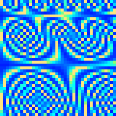
(a) Input dense $A$

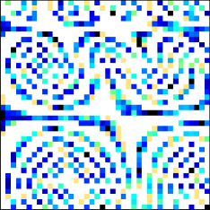
(b) Output sparse $X$

Figure 1: Input dense $A\in\mathbb{R}^{40\times 40}$, specified in Equation (11), and output sparse $X$ for $p=1$ and $q=0.8$. Plots generated using the cspy program [15] where darker pixel values correspond to larger magnitude.

Figure 2 shows the singular values of $A$ and $X$. Clearly, the lower end of the spectrum is perturbed less than the higher end. This shows that the algorithm is working as intended.

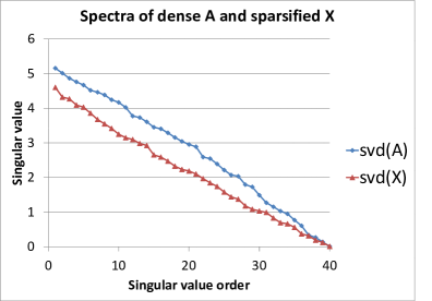
Figure 2: Singular values of $A$, specified in Equation (11), and $X$ for $p=1$ and $q=0.8$.

It is desirable to compute three quantities for measuring sparsification performance. First is the condition number of ${A}^{\dagger}X$ or $X{A}^{\dagger}$, second is the Frobenius norm difference of inverses, $\left|\left|{X}^{\dagger}-{A}^{\dagger}\right|\right|_{F}/\left|\left|{A}^{\dagger}\right|\right|_{F}$, and third is the number of non-zeros in $X$. The exact multiplication order in ${A}^{\dagger}X$ or $X{A}^{\dagger}$ is not particularly important. This is because almost always the two quantities are close to each other, as we have observed. Figure 3(a) shows how the condition number varies when we vary $q$ and $p$. Similarly, Figure 3(b) shows how the number of non-zeros change on varying the parameters. Note that for a fixed $q$, increasing $p$ leads to an increase in the number of non-zeros. The variation in condition number is reasonably smooth as long as not too many entries are discarded. An important measure of how much $X$ deviates from $A$ is the relative Frobenius norm difference of inverses. This is shown in Figure 4. The difference of inverses is important because our goal is to approximate the action of the inverse and not the operator itself.

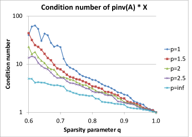
(a) Condition number of ${A}^{\dagger}X$

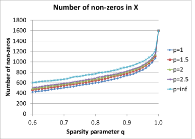
(b) Number of non-zeros in $X$

Figure 3: Effect of varying $p$ and $q$ on conditioning and sparsity. The input $A$ is specified in Equation (11).

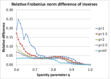
Figure 4: Effect of varying $p$ and $q$ on the relative Frobenius norm difference of inverses $\left(\left|\left|{X}^{\dagger}-{A}^{\dagger}\right|\right|_{F}/\left|\left|{A}^{\dagger}\right|\right|_{F}\right)$.

Based on the discussion above, it is natural to question which $p$ to choose. We argue that the precise value of $p$ is not important as long as one can change $q$ to achieve a given number of non-zeros. An evidence is shown in Figure 5 where we plot the data for various $p$ and $q$ values together. It shows that the conditioning and relative difference are highly correlated with the number of non-zeros rather than the exact $p$ and $q$ values. The “curves” for five $p$ values lie almost on top of each other when $q$ is varied in $[0.6,1]$.

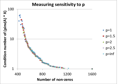
(a) $\text{cond}({A}^{\dagger}X)$

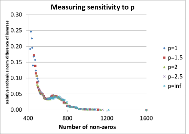
(b) $\left|\left|{X}^{\dagger}-{A}^{\dagger}\right|\right|_{F}/\left|\left|{A}^{\dagger}\right|\right|_{F}$

Figure 5: The figures show that the choice of $p$ is not too important if $q$ can be varied to achieve a specific amount of sparsity. Conditioning and relative difference of inverses is highly correlated with sparsity and not with parameters $p$ and $q$ individually.

We show that the computed $X$ is such that the eigenvalues of ${A}^{\dagger}X$, which are same as the eigenvalues of $X{A}^{\dagger}$, are clustered around a value near 1 on the real axis. See Figure 6(a) and (b) for eigenvalues of $A$, $X$, and ${A}^{\dagger}X$.

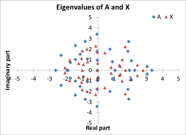
(a) Eigenvalues of $A$ and $X$

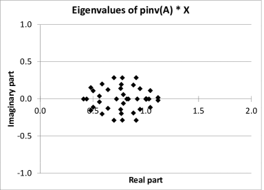
(b) Eigenvalues of ${A}^{\dagger}X$

Figure 6: Eigenvalues before and after sparsification. The clustered values in the second figure show that $X$ would perform well for preconditioning $A$ specified in Equation (11).

The last observation we have, which will be useful in the next paper, is that the non-zero entries of $X$ are highly correlated with the entries of $A$ at the preserved locations. Figure 7 shows the sorted entries of vectorized $A$ and the corresponding entries in $X$ for $p=1$ and $q=0.9$.

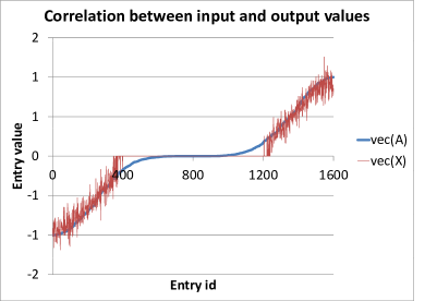
Figure 7: Correlation between $A$ and $X$ values after sorting vectorized $A$ and pairing corresponding $X$ entries with it.

Acknowledgements

This work was partially supported by the US Department of Energy SBIR Grant DE-FG02-08ER85154. The author thanks Travis M. Austin, Marian Brezina, Leszek Demkowicz, Ben Jamroz, Thomas A. Manteuffel, and John Ruge for many discussions.

References

- [1] C. Jhurani, Subspace-preserving sparsification of matrices with minimal perturbation to the near null-space. Part II: Approximation and Implementation, Submitted to Computers and Mathematics with Applications.
- [2] D. A. Spielman, N. Srivastava, Graph sparsification by effective resistances, in: Proceedings of the 40th annual ACM symposium on Theory of computing, STOC ’08, ACM, New York, NY, USA, 2008, pp. 563–568.
- [3] N. Halko, P. G. Martinsson, J. A. Tropp, Finding structure with randomness: Probabilistic algorithms for constructing approximate matrix decompositions, SIAM Rev. 53 (2) (2011) 217–288.
- [4] D. Achlioptas, F. Mcsherry, Fast computation of low-rank matrix approximations, J. ACM 54 (2).
- [5] S. Arora, E. Hazan, S. Kale, A fast random sampling algorithm for sparsifying matrices, in: Proceedings of the 9th international conference on Approximation Algorithms for Combinatorial Optimization Problems, and 10th international conference on Randomization and Computation, APPROX’06/RANDOM’06, Springer-Verlag, Berlin, Heidelberg, 2006, pp. 272–279.
- [6] T. M. Austin, M. Brezina, B. Jamroz, C. Jhurani, T. A. Manteuffel, J. Ruge, Semi-automatic sparse preconditioners for high-order finite element methods on non-uniform meshes, Journal of Computational Physics 231 (14) (2012) 4694 – 4708.
- [7] T. Austin, M. Brezina, T. Manteuffel, J. Ruge, Efficient Preconditioned Solution Methods for Elliptic Partial Differential Equations, Bentham Science Publishers, 2011, Ch. Automatic Construction of Sparse Preconditioners for High-Order Finite Element Methods.
- [8] A. Greenbaum, G. Rodrigue, Optimal preconditioners of a given sparsity pattern, BIT Numerical Mathematics 29 (1989) 610–634. doi:10.1007/BF01932737.
-
[9]
D. Ruiz, A scaling
algorithm to equilibrate both rows and columns norms in matrices, Tech.
rep., Rutherford Appleton Laboratory, Science and Technology Facilities
Council, UK (2001).
URL ftp://galahad.rl.ac.uk/pub/reports/drRAL2001034.pdf - [10] S. Beuchler, V. Pillwein, J. Schöberl, S. Zaglmayr, Sparsity optimized high order finite element functions on simplices, in: U. Langer, P. Paule (Eds.), Numerical and Symbolic Scientific Computing, Vol. 1 of Texts and Monographs in Symbolic Computation, Springer Vienna, 2012, pp. 21–44.
-
[11]
C. Jhurani, Multiscale modeling using
goal-oriented adaptivity and numerical homogenization, Ph.D. thesis, The
University of Texas at Austin (2009).
URL http://hdl.handle.net/2152/6545 - [12] S. P. Boyd, L. Vandenberghe, Convex Optimization, Cambridge University Press, 2004.
- [13] R. Bhatia, Matrix Analysis, Springer-Verlag, New York, 1997.
- [14] N. J. Higham, Accuracy and Stability of Numerical Algorithms, 2nd Edition, SIAM Books, Philadelphia, 2002.
- [15] T. A. Davis, www.cise.ufl.edu/research/sparse/SuiteSparse/.