Magnetohydrodynamic Modeling of the Solar Eruption on 2010 April 8

Abstract

The structure of the coronal magnetic field prior to eruptive processes and the conditions for the onset of eruption are important issues that can be addressed through studying the magnetohydrodynamic (MHD) stability and evolution of nonlinear force-free field (NLFFF) models. This paper uses data-constrained NLFFF models of a solar active region (AR) that erupted on 2010 April 8 as initial condition in MHD simulations. These models, constructed with the techniques of flux rope insertion and magnetofrictional relaxation, include a stable, an approximately marginally stable, and an unstable configuration. The simulations confirm previous related results of magnetofrictional relaxation runs, in particular that stable flux rope equilibria represent key features of the observed pre-eruption coronal structure very well and that there is a limiting value of the axial flux in the rope for the existence of stable NLFFF equilibria. The specific limiting value is located within a tighter range, due to the sharper discrimination between stability and instability by the MHD description. The MHD treatment of the eruptive configuration yields very good agreement with a number of observed features like the strongly inclined initial rise path and the close temporal association between the coronal mass ejection and the onset of flare reconnection. Minor differences occur in the velocity of flare ribbon expansion and in the further evolution of the inclination; these can be eliminated through refined simulations. We suggest that the slingshot effect of horizontally bent flux in the source region of eruptions can contribute significantly to the inclination of the rise direction. Finally, we demonstrate that the onset criterion formulated in terms of a threshold value for the axial flux in the rope corresponds very well to the threshold of the torus instability in the considered AR.

1. Introduction

The coronal source regions of solar eruptions (eruptive prominences, coronal mass ejections (CMEs), and flares) are characterized by low plasma beta, especially in active regions (ARs), where $\beta\sim 10^{-3}$ (Gary, 2001). Consequently, the magnetic field must remain nearly force free in the equilibrium sequence seen as the quasi-static evolution toward the onset of eruption. Since the energy needed to power the eruption can only be stored in coronal currents (Forbes, 2000) and since these currents tend to be strongly concentrated in the core of the source region (e.g., Sun et al., 2012), the pre-eruptive field is, to a good approximation, a nonlinear force-free field (NLFFF) obeying $\bm{\nabla}\bm{\times}\bm{B}=\alpha\bm{B}$ with the “force-free parameter” $\alpha(\bm{r})$ being a scalar function that varies across $\bm{B}$.

In order to understand the mechanism of eruptions and to quantify the criteria for their onset, knowledge of the field in the erupting coronal volume is required. However, the three-dimensional (3D) field structure is not amenable to measurement, and reliably inferring the coronal NLFFF from photospheric magnetograms has proven very difficult, even if vector magnetograms are available. Two strategies have been pursued. Extrapolation techniques solve the force-free equation numerically using a vector magnetogram as the bottom boundary condition. Several schemes produced reliable results when applied to test fields, in particular but not exclusively, the Grad-Rubin iteration, an optimization scheme, and magnetofrictional relaxation (MFR); see Schrijver et al. (2006) for an overview. However, it appears that the reconstruction of the coronal field from observed vector magnetograms matches reality closely only in a still relatively small number of cases; see especially Schrijver et al. (2008a), Canou & Amari (2010), Yelles Chaouche et al. (2012), Valori et al. (2012), and Sun et al. (2012). The methods had difficulty in producing reliable results for some other cases (e.g., Metcalf et al., 2008; Schrijver et al., 2008a; De Rosa et al., 2009). The violation of the force-free condition at the photospheric level in part of the magnetogram, uncertainties of the transverse magnetogram components, and the fragmentation of the flux in the photosphere down to sub-resolution scales are supposed to cause the problems which are not yet clearly understood.

The extrapolation technique has supported the modeling of eruptions as a flux rope instability (Török & Kliem, 2005; Kliem & Török, 2006) by computing stable and unstable coronal fields containing a flux rope (Valori et al., 2010) from magnetograms of the active-region model by Titov & Démoulin (1999). However, to date only few extrapolations of observed magnetograms have found a flux rope, see, e.g., Yan et al. (2001), Canou & Amari (2010), and Yelles Chaouche et al. (2012). A counterexample is the reconstruction of the highly nonpotential AR NOAA 11158, which did not yield a flux rope (Nindos et al. 2012; G. Valori 2013, private communication), although the subsequent violent eruption was suggestive of a flux rope eruption (Schrijver et al., 2011; Zharkov et al., 2011).

The flux rope insertion method (van Ballegooijen, 2004; van Ballegooijen et al., 2007) provides a viable alternative tool for the determination of the coronal NLFFF. Here a flux rope is inserted in the potential field computed from the vertical magnetogram component, to run at low height along the magnetogram’s polarity inversion line (PIL) in the section where a filament channel indicates a nearly horizontal, current-carrying field. This configuration is then numerically relaxed using magnetofriction (Yang et al., 1986). The resulting numerical equilibrium has received observational support in a growing number of cases by favorable comparison of various field line shapes (dips, arches of various shear angle relative to the PIL, S shape) and quasi-separatrix layers with coronal structures (Bobra et al., 2008; Su et al., 2009, 2011; Su & van Ballegooijen, 2012; Savcheva & van Ballegooijen, 2009; Savcheva et al., 2012c, a, b). In these studies, quiet-Sun or decaying active regions were modeled, where persistent shearing and flux cancellation make the formation of a coronal flux rope likely. It should be noted, however, that the method is not restricted to configurations containing a flux rope; the numerical relaxation can also result in an arcade configuration (Su et al., 2011).

The application of the flux rope insertion method led to the suggestion that the ratio between the magnetic flux in the rope, primarily the axial flux, and the unsigned flux in the AR may provide a new onset criterion for eruptions (Bobra et al., 2008). This has found considerable support in subsequent applications (see in particular Su et al., 2011) as well as in magnetohydrodynamic (MHD) simulations of flux cancellation (Aulanier et al., 2010; Amari et al., 2010), although the threshold may vary in a wide range (Savcheva et al., 2012b).

While the MFR method is well suited to find the dividing line between stability and instability in parameter space, it fails in correctly describing the dynamic evolution of unstable configurations because it represents a strongly reduced MHD description which disregards the inertia of the plasma and thus excludes the MHD waves. It is therefore of interest to study the relaxed or partially relaxed configurations in full MHD simulations. This allows further judgment of the obtained configurations by comparison with observations of erupting regions, and, additionally, an independent test of the marginal stability line in parameter space. The present investigation aims at carrying out the first such experiments.

Su et al. (2011, hereafter Paper I) performed extensive and detailed modeling of NOAA AR 11060 at the stage just prior to its eruption on 2010 April 8. The event included an erupting filament that evolved into a coronal mass ejection (CME) accompanied by a moderate flare. By varying the parameters of the inserted flux rope in a range of axial ($\Phi_{\mathrm{axi}}$) and poloidal ($F_{\mathrm{pol}}$) flux, the stability boundary in the $\Phi_{\mathrm{axi}}$–$F_{\mathrm{pol}}$ plane was determined with relatively high accuracy. Weakly twisted and arching field lines of a resulting stable configuration rather close to the stability boundary showed good correspondence to X-ray and EUV loops prior to the eruption. Low-lying highly sheared field lines of an unstable configuration rather close to the stability boundary corresponded well to the observed initial flare loops. A further result of high interest, with regard to the onset of eruptions, was that an X-type magnetic structure known as a hyperbolic flux tube (HFT; Titov et al., 2002; Titov, 2007) appeared at low heights under the flux rope when the axial flux was raised to approach the stability boundary. In the following we study a series of configurations from this investigation in the zero-beta MHD approximation. The configurations are arranged on a path in the $\Phi_{\mathrm{axi}}$–$F_{\mathrm{pol}}$ plane that crosses the stability boundary and include the models which compare favorably to the observations.

The simulations also allow us to compare the conditions at the onset of instability with the ratio of rope and ambient flux (Bobra et al., 2008) and with the height profile of the flux rope’s ambient field (van Tend & Kuperus, 1978; Kliem & Török, 2006). Identification of the conditions necessary for instability is a key goal of this research.

Section 2 presents a summary of the observations from Su et al. (2011). This is followed by a detailed description of the numerical model in Sections 3 and 4. The relaxation of stable configurations and the eruption of an unstable configuration are presented in Sections 5 and 6, respectively. Our conclusions are given in Section 7.

2. Summary of Observations

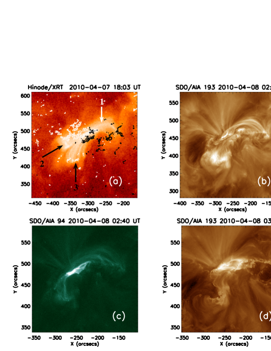
Figure 1.— Structure of AR 11060 before and during the eruption observed by (a) Hinode/XRT, and (b)–(d) SDO/AIA. In panel (a) the contours refer to the photospheric line of sight (LOS) magnetogram taken by the Helioseismic and Magnetic Imager (HMI; Schou et al., 2012) on SDO at 02:00 UT on 2010 April 8 (white: positive; black: negative; see Figure 2 for a more detailed contour plot). The coronal loops in the core of the region are organized in three sets, labeled as 1–3 and discussed in the text. (A color version of this figure is available in the online journal.)

The event under study originated in AR 11060 on 2010 April 8 around 02:30 UT. It included an eruptive prominence that evolved into a CME, a two-ribbon solar flare of GOES class B3.7, prominent coronal dimmings, and a coronal EUV wave. The eruption was observed on disk by the Atmospheric Imaging Assembly (AIA, Lemen et al., 2012) on the Solar Dynamics Observatory (SDO) and by the X-Ray Telescope (XRT, Golub et al., 2007) on the Hinode mission. The Extreme Ultraviolet Imager (EUVI) and the coronagraphs COR1 and COR2 (Howard et al., 2008) aboard the Solar-Terrestrial Relations Observatory (STEREO) Ahead spacecraft saw the event nearly exactly at the east limb. A detailed description of these data including animations can be found in Paper I. Additional information is given in the analysis of the EUV wave (Liu et al., 2010) and of the possible occurrence of the Kelvin-Helmholtz instability at the surface of the expanding flux (Ofman & Thompson, 2011).

Figure 1 shows Hinode/XRT (a) and SDO/AIA (b) images of AR 11060 before the eruption. The core of this active region contains three sets of coronal loops as shown in Figure 1(a). The set of loops labeled 1 is located in the northwestern part of the region (white arrow). Loop sets 2 and 3 are associated, respectively, with the major positive polarity (white contours) in the northeast of the region and with a group of minor positive flux patches in the southeast (both marked by black arrows). The combined loop sets 1 and 2 yield a slightly sigmoidal appearance at soft X-rays. Figure 1(b) shows a thin, dark filament following mainly the highly sheared loop set 2, i.e., located between loop sets 1 and 3.

The eruption began around 02:10 UT with motion of material along this filament in the southeastward direction (as seen by AIA) and nearly horizontally (as seen by EUVI-A on STEREO Ahead). About 18 minutes later, the filament began to lift off. From about 02:33 UT, the overlying loops are seen to rise in the EUVI-A 195 Å images. The first flare brightenings appear in AIA 94 Å images on either side of the erupting filament around 02:30 UT, and the GOES soft X-ray emissions commence near 02:45 UT. Thus, the onset of upward flux expansion, which evolved into the CME, and the onset of the flare brightenings occurred in close temporal and spatial association.

Initially highly sheared flare loops became visible between 02:30 and 02:40 UT in the AIA 94 Å channel (Figure 1(c)), they connected the first flare brightenings in the strong-field section of the PIL. The typical evolution toward lower shear was seen in the loops forming subsequently (Figure 1(d)). These observations indicate that the component of the magnetic field along the PIL points northwestward and that the field has positive helicity, consistent with the forward S shape of the combined loop sets 1 and 2. The brightenings early in the flare (Figure 1(c)) as well as the subsequent equatorward growth of the CME dimmings yield an overall inverted U shape of the parts of the region actively involved in the eruption. This is similar to the combined loop sets 1 and 3 and suggests that their flux is an integral part of the eruption, although loop set 3 connects to a minor flux area in the magnetogram.

The erupting flux took a strongly inclined path toward the equator, initially at about $45^{\circ}$ from vertical, then developing an even more inclined southward expansion in the low corona imaged by EUVI-A, and finally turning into a more radial propagation near the equatorial plane, as imaged by the COR2-A coronagraph. The EUVI data do not reveal the rise profile of the erupting filament, as the material very quickly lost contrast in the 195 Å channel and the cadence of the other channels was too low. However, the rise velocity of overlying coronal loops can be estimated and is found to reach about 170 km s^-1 within the EUVI-A field of view (see Section 6.1). The CME reached a median projected speed of $\approx 520$ km s^-1 in the COR2-A field of view, as quoted in the CACTus CME Catalog (Robbrecht et al., 2009).

3. Magnetofrictional Modeling

The presence of highly sheared loops (Figure 1) indicates that the coronal magnetic field in the observed region deviates significantly from a potential field. In Paper I we used a set of codes, called the Coronal Modeling System (CMS), to construct non-potential field models of the observed region. The methodology involves inserting a thin magnetic flux rope into a three-dimensional (3D) potential-field model along a specified path, and then applying magnetofrictional relaxation (MFR) (Yang et al., 1986; van Ballegooijen et al., 2000) to produce either a non-linear force-free field (NLFFF) model or unstable model, depending on the magnitude of the inserted flux. MFR refers to an evolution of the magnetic field $\bm{B}(\bm{r},t)$ in which the medium is assumed to be highly conducting and the plasma velocity $\bm{v}$ is proportional to the Lorentz force $\bm{j\times B}$, where $\bm{j=\nabla\times B}$ is the current density. The resulting 3D magnetic models are based on observed photospheric magnetograms and therefore accurately represent the lower boundary conditions on the magnetic field in the flaring active region. This makes such models ideally suited as initial conditions for 3D MHD simulations.

In this paper, we use flux rope insertion and MFR to produce initial conditions for a 3D MHD code, which is described in Section 4. One problem is that the MHD code assumes Cartesian geometry, whereas the CMS codes use spherical geometry, and the considered area is too large to ignore curvature effects. Therefore, we cannot simply interpolate the relevant models from Paper I. Instead, the methods used in Paper I are modified in several ways, as described in the following. First, we construct a map of $B_{r}(\theta,\phi)$, the radial component of magnetic field at the solar surface ($r=R_{\odot}$) in and around the observed AR. The map is based on an SDO/HMI magnetogram taken at 2:00 UT. The map is computed by interpolating the observed LOS field onto a longitude-latitude grid, and then dividing by the cosine of the heliocentric angle to obtain $B_{r}$. This original map has $384\times 384$ cells and covers an area of $41.3^{\circ}$ in longitude by $36.8^{\circ}$ in latitude, centered on the observed AR. Then the spatial scale of the map is reduced, and the center of the map is displaced to the equator, corresponding to a reduction in scale by a factor $f=16.97$. The rescaled map covers only $2.2^{\circ}$ in longitude and latitude, which is sufficiently small that the resulting spherical models can be treated as if they were Cartesian.

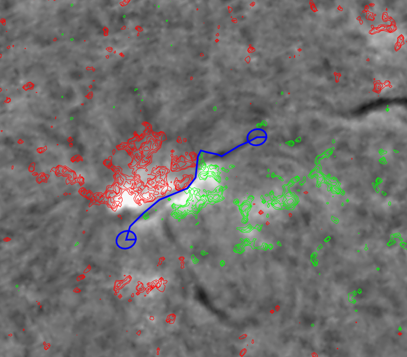
Figure 2.— H$\alpha$ image of the observed active region, obtained at Kanzelhöhe Solar Observatory on 2010 April 8 at 9:00 UT. The red and green contours show the radial photospheric magnetic field component derived from the SDO/HMI LOS magnetogram taken at 2:00 UT. The blue curve shows the path of the inserted flux rope between the marked end points. (A color version of this figure is available in the online journal.)

In CMS the magnetic field is described using two spatial grids: a high resolution grid (HIRES) covering the target region and its local surroundings, and a low resolution grid covering the entire Sun. The non-potential field in the HIRES region is described in terms of vector potentials ($\bm{B=\nabla\times A}$). In the standard approach, the global grid is used for a potential field source surface (PFSS) model; its main purpose is to improve the side boundary conditions for the HIRES domain. However, for the scaled models used here the global grid can no longer be used. Instead we assume that the normal component of magnetic field vanishes at the side boundaries of the HIRES domain ($B_{\theta}=0$ and $B_{\phi}=0$ at the latitudinal and longitudinal boundaries, respectively). These boundary conditions imply that the net flux entering the domain through the lower boundary is also present at larger heights, and leaves the domain through the outer boundary. We found that small flux imbalances between positive and negative magnetic fluxes in the imposed magnetic map ($B_{r}$) can produce fields at large heights that are dominated by such “monopole” components. Furthermore, in preliminary MHD simulations we found that such monopolar fields can inhibit the eruption of low-lying flux ropes. Therefore, in the present paper we correct the flux imbalance in $B_{r}(\theta,\phi)$ at the lower boundary. The photospheric fluxes are balanced by subtracting a spatially constant value of about 2.2 Gauss from $B_{r}(\theta,\phi)$, except near the border of the computational domain where $B_{r}$ is set to zero.

The next steps are to select the path of the flux rope, compute a potential field, and insert the flux rope into the 3D magnetic model. The path should follow the PIL of the AR; we use the same path as in Paper I. Figure 2 shows the selected path superposed on a H$\alpha$ image obtained at Kanzelhöhe Solar Observatory at 9:00 UT. The red and green contours indicate the photospheric flux distribution $B_{r}(\theta,\phi)$ before scaling.

In this paper, we construct three different models with the same flux rope path, height, and cross section, but with different values of the axial flux of the flux rope. The axial fluxes before scaling are $\Phi_{\mathrm{axi}}=4\times 10^{20}$, $5\times 10^{20}$ and $6\times 10^{20}$ Mx, which were chosen because these values appear to straddle the stability boundary (see Paper I). After scaling these axial fluxes are reduced by the square of the scaling factor. The axial flux is inserted into the 3D model as a thin flux tube that is elevated above the photosphere. At the ends of the tube (indicated by circles in Figure 2), the flux of the tube is connected to surrounding sources on the photosphere. Poloidal fields are added by wrapping flux rings around this tube. The assumed poloidal flux is $F_{\mathrm{pol}}=10^{10}$ Mx cm^-1 (before reduction by the scaling factor). For more details on how the flux rope is inserted into the 3D models, see Su et al. (2011) and references therein.

The next step is to apply 30,000 iterations of MFR to each of the three models. This drives the magnetic field toward a force-free state (if one exists) or causes the field to slowly expand (if the configuration is unstable). Each 3D magnetic model is then resampled on the grid used by the MHD code. This grid is nonuniform in longitude, latitude and height; it provides high spatial resolution in the center of the AR and gradually reduced resolution farther away from the center. Figure 3 shows vertical cross-sections through the three models after resampling on the Cartesian grid. For consistency with the designation in Paper I we will refer to the axial flux values of the inserted flux ropes corresponding to the magnetogram size before the spatial scaling, $4\times 10^{20}$, $5\times 10^{20}$ and $6\times 10^{20}$ Mx. The first panel indicates on a magnetic map at height 4.2 Mm where the vertical cross-sections are taken. The quantity plotted in the three other panels is $\alpha=\bm{j\cdot B}/B^{2}$, which is a measure of the parallel electric current. Note that the currents are concentrated near the edge of the flux rope, and that the height of the flux rope increases with axial flux. Higher axial flux implies higher total current running along the flux rope, which in turn implies a stronger upward force on the current-carrying flux. This force can be described as a repelling force between the flux rope current and its subphotopheric image if the flux rope runs nearly parallel to the solar surface (Kuperus & Raadu, 1974) and, equivalently, as the hoop force on the rope if the rope arches upward considerably (Démoulin & Aulanier, 2010). Consequently, the equilibrium height increases with increasing axial flux. $\alpha$ is positive across essentially the whole cross section of the flux rope, i.e., the field is right handed and the rope carries nearly no return current. Both models with $\Phi_{\mathrm{axi}}\geq 5\times 10^{20}$ Mx possess an X-type magnetic structure—an HFT—running at low height under the flux rope (see Paper I for detail).

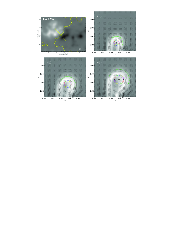
Figure 3.— The three configurations investigated in this paper after 30 000 MFR iteration steps. Shown are: (a) the magnetogram $B_{z}(x,y)$ at a height of $z=4.2$ Mm, the PIL at this height, and the position of a vertical plane used in the analysis; the plane is placed perpendicular to the PIL such that it passes very near the apex point of the rope’s magnetic axis for all configurations. (b)–(d) Force-free parameter $\alpha$ and in-plane magnetic field vectors in this diagnostics plane (for $z\geq 4.2$ Mm; $s$ denotes horizontal distance). The configurations possess axial flux of 4, 5, and $6\times 10^{20}$ Mx for (b)–(d), respectively, and an identical poloidal flux of $10^{10}$ Mx cm^-1. Lengths are given in $R_{\odot}/f$, i.e., they would correspond to a unit of $1R_{\odot}$ if scaled back to the original magnetogram size. The gray background in these panels corresponds to $\alpha=0$, and in the area shown $\alpha$ lies in the range $[-9,141]$, $[-8,125]$, and $[-8,118]$ for panels (b)–(d), respectively. Crosses show the initial position of the fluid elements used as start points of the field line tracing in the subsequent plots and animations; the trajectories of these fluid elements are followed through the simulations. Rainbow-colored crosses are placed inside the FR near its edge, and green crosses are placed in the inner part of the overlying flux. The plus signs mark the apex point of the flux rope’s magnetic axis. The motion of this fluid element is used to generate the rise profiles in Figures 6, 8, and 14. (A color version of this figure is available in the online journal.)

By applying the MFR much longer, Su et al. concluded in Paper I that, for the given value of $F_{\mathrm{pol}}=10^{10}$ Mx cm^-1, the model with $\Phi_{\mathrm{axi}}=5\times 10^{20}$ Mx lies near the stability boundary in the $\Phi_{\mathrm{axi}}$–$F_{\mathrm{pol}}$ plane. All configurations with $\Phi_{\mathrm{axi}}\leq 4.5\times 10^{20}$ Mx relaxed to an apparently stable and approximately force-free state in 30,000 MFR iterations, while all configurations with $\Phi_{\mathrm{axi}}\geq 6\times 10^{20}$ Mx did not relax, rather the inserted flux rope continued to rise.

4. Magnetohydrodynamic Modeling

In the MHD modeling, the configurations obtained after 30,000 magnetofrictional iterations are used as the initial condition, $\bm{B}_{0}(\bm{r})$, for the numerical integration of the compressible ideal MHD equations in the zero-beta limit. We set the initial velocity to zero, $\bm{u}_{0}=0$, and choose $\rho_{0}(\bm{r})=B_{0}(\bm{r})^{3/2}$ as model for the initial density. This implies a gradual decrease of the initial Alfvén velocity $V_{\mathrm{A0}}=B_{0}(2\mu_{0}\rho_{0})^{-1/2}$ with distance from the strong field in the core of the active region, such that the height profile $V_{\mathrm{A0}}(z)$ approximately follows the empirical height profile in Vršnak et al. (2002, their Figure 5). Such a choice of $\rho_{0}(\bm{r})$ generally yielded good quantitative matches with observed CME rise profiles in previous simulations (e.g., Török & Kliem, 2005; Schrijver et al., 2008b; Kliem et al., 2012).

The equations used and the numerical scheme are detailed in Török & Kliem (2003). The condition $\beta=0$ decouples the energy equation from the system. Gravity can be neglected for both purposes of the simulations in this paper: further relaxation of stable force-free configurations and the study of CME acceleration in a region of relatively strong magnetic field (an AR) in the case of instability. Numerical diffusion breaks the frozen-in condition when thin layers of inhomogeneous field (i.e., high current densities) develop, thus allowing magnetic reconnection. The equation of motion includes a viscous term solely to ensure numerical stability.

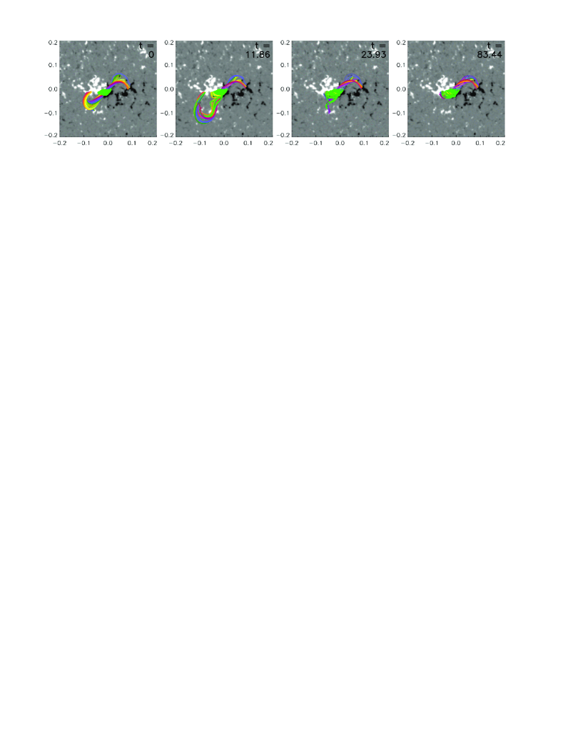
Figure 4.— Stages in the relaxation of the model with $\Phi_{\mathrm{axi}}=4\times 10^{20}$ Mx. Shown are field lines in vertical view and the magnetogram $B_{z}(x,y,0,t)$ with the gray scale saturated at one tenth of the peak value. Rainbow-colored field lines lie in a flux shell slightly inside the boundary of the flux rope and green field lines visualize the inner part of the overlying flux (see Figure 3). (A color version of this figure is available in the online journal.)

Careful attention is paid to the amount of numerical diffusion in the integration. We use a modified verson of the two-step Lax-Wendroff scheme that replaces the stabilizing but very diffusive Lax term in the auxiliary step of the iteration by so-called artificial smoothing (Sato & Hayashi, 1979; Török & Kliem, 2003). While the Lax term replaces the value of the integration variable by the average of the values at the six neighboring grid points, the artificial smoothing replaces only a fraction of the value, $\sigma\ll 1$, by the average at the neighboring points. For the magnetic field, this averaging is switched off completely in the relaxation runs ($\sigma_{B}=0$) to minimize any slow diffusive change of the force-free equilibrium, improving the convergence toward the equilibrium. The eruption of the unstable configuration can be followed with the same setting; however, a parametric study of the field smoothing yields the most reliable numerical results and best numerical stability if a small level of smoothing, $\sigma_{B}\sim 10^{-3}$, is adopted in the volume under the rising flux rope, where a vertical current sheet develops (see Section 6 for detail). This operation is not applied in the bottom layer of the box, $\{z=0\}$, so that there is no diffusion of the field in the magnetogram plane.

Minimizing the numerical diffusion in the momentum equation allows us to capture any residual forces that result from our initial conditions being out of equilibrium. We have experimented with the values of $\sigma_{u}$ and $\nu$ (the coefficient of viscosity), and chosen them as close to the limit of numerical stability as reasonably possible, i.e., a lowering of either of them by a factor of 2 would lead to numerical instability in the course of the simulation run. Best numerical stability is obtained by smoothing the density at the same level. In the main volume of the box $\sigma_{\rho}=\sigma_{u}=0.005$. A gradual enhancement of the smoothing toward the bottom boundary, by a factor two, is necessary to allow stable integration in the presence of the strong flux gradients in the magnetogram and their associated currents. Uniform small viscosity is chosen: $\nu=0.002$ (after normalization).

The integration volume corresponds to $0.72R_{\odot}\times 0.72R_{\odot}\times 1R_{\odot}$ when the magnetogram is scaled back by the factor $f$ to the original edge length. This volume is discretized by a Cartesian grid with uniform resolution of $0.002R_{\odot}$ (1.9 arcsec) in the AR and its immediate surroundings ($|x|<0.1R_{\odot}$, $|y|<0.1R_{\odot}$, $z<0.2R_{\odot}$) and a gradually increasing spacing in the outer parts, reaching $0.0065R_{\odot}$ at the side boundaries and $0.015R_{\odot}$ at the top. Closed boundaries are implemented at the sides and top of the volume by keeping the velocity at zero, including the first inner grid layer, so that the field vector in the boundary layers does not change. At the bottom boundary the velocity is kept at zero in the magnetogram plane, $\bm{u}(x,y,0,t)=0$, which ensures that the normal magnetogram component $B_{z}$ keeps its initial values, but allows the transverse components to change, either to approach an NLFFF, or to consistently evolve with an eruption.

The box height ($1R_{\odot}$) is chosen as the length unit. The field strength is normalized by the peak value, $\max(B_{0})=955$ Gauss, which lies in the magnetogram plane. Velocities are normalized by the peak value of the initial Alfvén velocity, $\hat{V}_{\mathrm{A0}}$, whose location coincides with the location of the highest field strength. The initial Alfvén velocity in the body of the flux rope is about half this value. Time is normalized by the corresponding Alfvén time $\tau_{\mathrm{A}}=R_{\odot}/\hat{V}_{\mathrm{A0}}$.

5. Relaxation of Stable and Nearly Marginally Stable Configurations

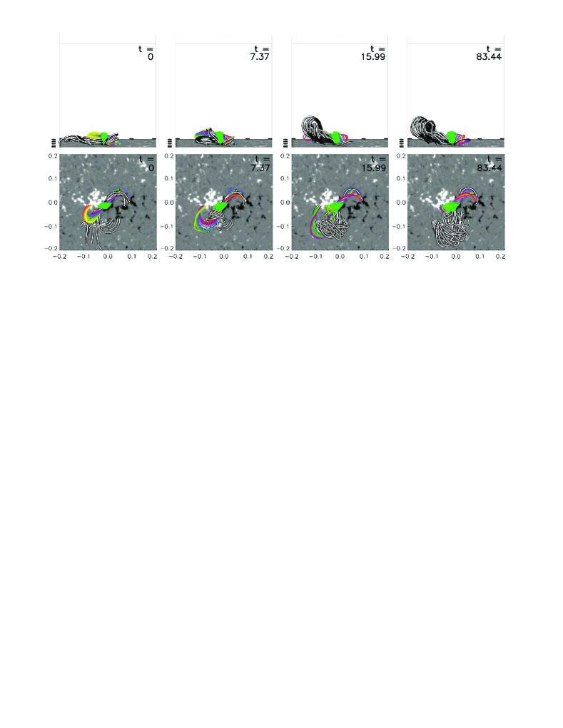
Figure 5.— Same as Figure 4 but with additional field lines traced from a set of fixed points located at $z=0$ in the minor positive flux concentration in the southeast of the active region. The strong interaction of this flux with the inserted rope leads to the southward bulging of the rope and to multiple reconnections involving the splitting and the subsequent recovery of a single rope. The upper row shows the cube above the selected magnetogram area in perspective views oriented in $-x$ direction. (A color version and an animation of this figure are available in the online journal.)

Figure 6.— Height-time and velocity-time profile showing the relaxation of the model with $\Phi_{\mathrm{axi}}=4\times 10^{20}$ Mx. The fluid element initially located at the estimated apex point of the flux rope’s magnetic axis, shown in Figure 3 by a plus sign, is followed. The solid lines show the distance $d(t)$ from the initial projection of the apex onto the bottom plane and the 3D velocity of the fluid element, $|\bm{u}(t)|$. The dashed lines show the height above the bottom plane and $u_{z}(t)$. Dotted lines in the logarithmic plot show downward velocities ($|u_{z}(t)|$ for $u_{z}<0$).

In our MHD description both models with $\Phi_{\mathrm{axi}}\leq 5\times 10^{20}$ Mx are found to relax to a stable force-free equilibrium (NLFFF). As expected, the relaxation proceeds faster and deeper for the model with $\Phi_{\mathrm{axi}}=4\times 10^{20}$ Mx; nevertheless, the initial configuration clearly includes a small level of residual forces and the flux rope experiences further reconnection with the ambient field in the course of the relaxation. The overall evolution is characterized in Figure 4. From the field line plot at $t=0$ it is clear that the eastern part of the inserted flux rope has evolved significantly in the course of the MFR: the flux connected from the end point of the path shown in Figure 2 to the main positive polarity in the northeast of the region (i.e., in the direction of loop set 2 in Figure 1) now bulges out to the south in the direction of loop set 3. Close similarity to loop set 1 on the western side was achieved with relatively little change. The strong evolution of the eastern part continues in the course of the MHD relaxation, driven primarily by reconnection with the minor positive polarity in the southeast of the region. This wraps flux from the minor polarity around the flux rope, passing northward under the rope and from there arching over the rope toward the main negative polarity in the west. The bulging of the southern part of the rope is thus considerably enhanced. As a consequence, the flux rope reconnects with the perturbing flux and its whole eastern elbow splits.

This interaction with the ambient flux rooted in the minor positive polarity is shown in more detail in Figure 5 ($t=0\mbox{--}16\tau_{\mathrm{A}}$) and its accompanying animation. Further reconnection in this area subsequently simplifies the structure of the inserted flux which returns to an essentially unsplit flux rope, shorter on the eastern side, where it now displays closer similarity in shape with loop set 2 (Figures 4–5 at $t>20\tau_{\mathrm{A}}$). New low-lying connections run from the minor positive polarity to the eastern part of the main negative polarity under the main body of the relaxed flux rope (Figure 5 at $t=83\tau_{\mathrm{A}}$); these are similar to loop set 3. Note that these connections differ from the ones at $t=0$. Their existence is not even indicated in the potential field. Additionally, new high-arching field lines extend from the minor positive polarity with a dominant east-west orientation. They have absorbed some of the twist of the inserted flux. One can speculate that such higher field lines confine plasma of lower density, so that these connections should be less visible in X-ray and EUV images. Some irregularly shaped emission does exist in this area at the temperature ($T\approx 1.5$ MK) sampled by the AIA 193 Å channel (Figure 1(b)). It consists of moss essentially cospatial with the minor flux concentration and of weak diffuse emission slightly southward, which has a dominantly east-west orientation reminiscent of the high-arching field lines seen in the simulation from $t\sim 15\tau_{\mathrm{A}}$ onward.

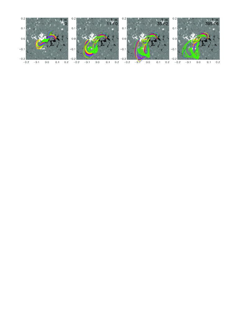
Figure 7.— Stages in the relaxation of the model with $\Phi_{\mathrm{axi}}=5\times 10^{20}$ Mx in the same format as Figure 4. (A color version and an animation of this figure are available in the online journal.)

More quantitative information about the relaxation, displayed in Figure 6, is obtained by monitoring the position and velocity of the fluid element initially at the apex point of the rope’s magnetic axis (marked by a plus sign in Figure 3). We first note a minor but quick shift in apex height at the very beginning of the run ($t\lesssim 2\tau_{\mathrm{A}}$), which potentially results from two effects. One reason lies in the difference between the codes in obtaining the current density. While the MFR code runs on a staggered grid, the MHD code iterates all variables at the same positions, leading to differences in derived quantities between the codes which increase with degrading spatial resolution. Since all models include a relatively thin layer of enhanced current density at the edge of the flux rope which is resolved by only $\sim 5\mbox{--}10$ grid cells (Figure 3), the Lorentz force differs somewhat between the MFR and MHD descriptions in this critical layer, and so does the equlibrium height of the flux rope. It is clear, however, that the overall difference in the volume of the flux rope must be moderate at the resolution employed: the height of the flux rope’s apex increases by only 15% (from $h_{0}=0.025$ to $h(t\!=\!2)=0.029$). Stronger differences exist in the first few grid layers above the magnetogram, where the strong fragmentation of the flux is not fully resolved, resulting in small volumes of high current density. Although the associated Lorentz forces do not have a coherent direction, they may still contribute to the change in equilibrium height. This contribution can be estimated through a comparison with the relaxation behavior of the potential field, calculated on the spherical grid of CMS and resampled on the Cartesian grid of the MHD code in the same manner as the three AR models. The fluid element at the same initial position as the one considered in Figure 6 rises by only 2.1% to $h=0.0255$, also experiencing most of this displacement (80%) within the first two Alfvén times. Thus, the contribution from discretization errors in the current density near the bottom of the box appears to be only minor. Second, part of the initial rise may be due to the status of relaxation after the 30,000 MFR iterations. Although already deep, as the subsequent rapid decrease of the velocities shows, it is obviously not yet complete (see above). The low level of viscosity and velocity smoothing in the MHD relaxation allows the small residual forces to build up a noticeable velocity in the motion to the stable equilibrium height.

Subsequently, a further rise to $h=0.033$ occurs which is associated with the reconnections discussed above. The velocity of the fluid element shows a nearly monotonic decrease, with a weak transient enhancement during $t\sim(5\mbox{--}20)\tau_{\mathrm{A}}$ related to the southward bulging of the flux rope. Following the initial jump (i.e., after $t\approx 2\tau_{\mathrm{A}}$), the vertical velocity falls by more than three orders of magnitude to $u_{z}\sim 10^{-6}~{}\hat{V}_{\mathrm{A0}}$, which is a clear signature that the flux rope relaxes deeply. To further quantify the relaxation, we compute the current-weighted average sine of the angle between current and magnetic field, $\sigma_{j}=\sum_{i}j_{i}\sigma_{i}/\sum_{i}j_{i}$, where $\sigma_{i}=|\bm{j}_{i}\bm{\times B}_{i}|/(B_{i}j_{i})$ and the index $i$ runs over all grid cells. Following standard practice in the use of this quantity in magnetogram extrapolations (e.g., De Rosa et al., 2009), the outer parts of the box are excluded. Additionally, we exclude the first three grid layers at the bottom of the box, where the strong fragmentation of the flux is not fully resolved. Their contribution raises the value of $\sigma_{j}$ by about an order of magnitude, while the outer parts of the box contribute only a further factor of $\approx\!1.2$. In the volume $|x|<0.2$, $|y|<0.2$, $0.006<z<0.4$ we find $\sigma_{j}(0)=0.066$ and $\sigma_{j}(t\!=\!83)=0.015$, falling monotonically, except for a moderate enhancement during $t\sim(5\mbox{--}20)\tau_{\mathrm{A}}$. Here it should be kept in mind that the initial degree of force freeness, $\sigma_{j}(0)$, is degraded from the MFR relaxation result by the transition from the staggered CMS grid to the non-staggered grid of the MHD code. The magnetic energy in the box decreases by 2.7% in the course of the relaxation.

Figure 8.— Height-time and velocity-time profile showing the relaxation of the model with $\Phi_{\mathrm{axi}}=5\times 10^{20}$ Mx in the same format as Figure 6.

The model with $\Phi_{\mathrm{axi}}=5\times 10^{20}$ Mx follows a rather similar evolution in the course of its relaxation, albeit on a much longer time scale and relaxing somewhat less deeply (Figures 7 and 8). In particular, the reconnection of the inserted flux rope with the minor positive flux concentration in the southeast of the AR yields a similar bulging, splitting, and subsequent trend of recovery. The resulting relaxed state is largely similar, but here the flux rope remains partly split. Again, the major part of the relaxed rope matches the observed loop sets 1 and 2 relatively well. The split-off part of the rope and some of the new connections between the minor positive polarity and the main negative polarity correspond well to loop set 3. Finally, diffuse, high-arching loops, with a dominant east-west orientation, are formed south of the minor positive polarity, as in the model with less axial flux. A noteworthy difference is the higher initial displacement of the flux rope by $\approx 50\%$ from $h_{0}=0.036$ to $h(2)=0.053$ in the first $\approx 2\tau_{\mathrm{A}}$. It can be seen in Figure 3 that the resolution of the current layer at the surface of the flux rope in the two models is rather similar, so the stronger initial displacement must be primarily due to a less complete relaxation in the course of the MFR. Indeed, we find $\sigma_{j}(0)=0.074$, slightly higher than for the model with $\Phi_{\mathrm{axi}}=4\times 10^{20}$ Mx. Except for a moderate enhancement during $t\sim(5\mbox{--}15)\tau_{\mathrm{A}}$, the average angle between $\bm{j}$ and $\bm{B}$ decreases monotonically to $\sigma_{j}(t\!=\!83)=0.019$ and $\sigma_{j}(t\!=\!395)=0.012$.

After about $100\tau_{\mathrm{A}}$ the residual velocities lead to a very slow rise of the flux rope position, hardly visible in the field line plots but obvious in Figure 8. It is difficult to judge whether this evolution is part of the relaxation or due to of a diffusive drift of the equilibrium in the long computation comprising of slightly over $10^{6}$ iteration cycles. Animated field line plots (Figure 7) show that the rope continues to evolve over this long time period (some of the field lines change their photospheric connections considerably), and on average the velocity of the rope continues to decrease (apart from episodic enhancements); both properties suggest that the slow drift may be part of the relaxation. Nevertheless, it is unclear whether continuing this run can lead to further understanding of this model free from numerical effects, so the run was terminated. Adopting the scaling of the simulation in Section 6.1, the nearly 400 Alfvén times of this relaxation correspond to up to 2.3 days, longer than the equilibrium can be assumed to be static. By the end of the relaxation, the magnetic energy in the box has dropped by 4.5%. The model appears stable in the MHD treatment, but is doubtlessly much closer to the point of marginal stability than the previous model.

Figure 9.— Evolution of the model with $\Phi_{\mathrm{axi}}=5\times 10^{20}$ Mx following a strong perturbation applied at a stage of deep relaxation ($t=123\tau_{\mathrm{A}}$). Position and velocity of the fluid element at the apex of the flux rope are plotted in the same format as in Figure 8, with the 3D position $d(t)$ here referenced to the bottom projection of the apex point at $t=123\tau_{\mathrm{A}}$.

To further test for the stability of this model, we have perturbed it at the times of apparently deepest relaxation, $t=123\tau_{\mathrm{A}}$ and $t=395\tau_{\mathrm{A}}$. The flux rope was raised to $h\approx 0.105$ by prescribing upward velocities at the apex in a sphere of radius equal to the minor flux rope radius for $15\tau_{\mathrm{A}}$. Slightly below this height the unstable third model starts its fast ascent (see next section). Despite the very strong distortion, the flux rope returned close to the original position, executing quickly decaying relaxation oscillations. This is shown in Figure 9 for the perturbation applied at $t=123\tau_{\mathrm{A}}$. Nearly identical behavior results for the perturbation applied at the end of the relaxation run. These tests support the interpretation that the model with axial flux $\Phi_{\mathrm{axi}}=5\times 10^{20}$ Mx relaxes to a stable equilibrium.

The model can be driven to eruption by further flux cancellation. This was tested by prescribing horizontal flows converging toward the PIL in the strong-flux section of the PIL and allowing for diffusion of the field in the vicinity of the PIL, analogous to the diffusion in Aulanier et al. (2010) and Amari et al. (2011). Cancellation of about 10% of the unsigned flux in the region caused the eruption of the flux rope (but more extended experimenting might find eruption at an earlier stage). Different from observation, the flux rope took a nearly vertical path. This and the fact that an appropriate modeling of pre-eruption driving by flux cancellation should start from a magnetogram taken at an earlier time, led us to reserve a more detailed investigation of such simulations for a future study.

6. Eruption of the Unstable Configuration

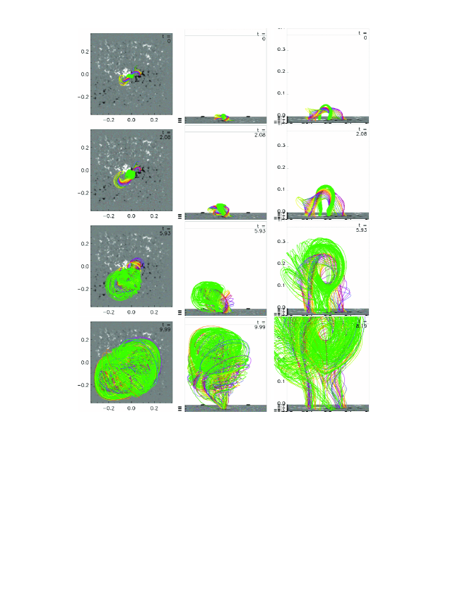
Figure 10.— Flux rope eruption in the model with $\Phi_{\mathrm{axi}}=6\times 10^{20}$ Mx. The format is similar to Figures 4 and 7. The whole box is shown in the left two columns. The eruption starts strongly inclined, as observed. Subsequently, the erupting flux is deflected at the closed side boundary. Originally overlying flux (green field lines) is strongly reconnected into the rope by flare reconnection in the vertical current sheet that forms under the rope (see Figure 11). (A color version and an animation of this figure are available in the online journal.)

Similar to the result of the MFR in Paper I, the rope with axial flux $\Phi_{\mathrm{axi}}=6\times 10^{20}$ Mx does not relax to an equilibrium, but rather erupts. As expected, the initial configuration deviates stronger from force freeness than the two stable models, $\sigma_{j}(0)=0.083$. The evolution starts with a rapid displacement of the rope within the first two Alfvén times, comprising the lifting of the middle part and the southeastward expansion of the eastern elbow, which are very similar to the initial behavior in the relaxation runs of the previous section. The interaction with the flux rooted in the minor positive polarity is also similar but does not lead to a split rope (which occurs at $t>5\tau_{\mathrm{A}}$ in the relaxation runs) because of the commencing eruption.

A seamless transition to an initially slower but accelerating rise follows, leading to the eruption of the whole flux rope (see Figure 10 and the accompanying animation). The main direction of this motion is upward and southward, initially (at $t=2\tau_{\mathrm{A}}$) at an inclination of 40^∘–45^∘ to the vertical, which is very close to the observed direction. Interaction with a nearby coronal hole (Gopalswamy et al., 2009) and asymmetry of the photospheric flux distribution (Panasenco et al., 2013) have been proposed to cause deviations from radial ascent. The former is not included in our model, while the latter effect is present, but presumably not very strong: the main positive polarity in the AR contains only $\approx 10\%$ more flux than the main negative polarity. However, the positive polarity is more compact. An additional effect is suggested by the shape of loop sets 1 and 3: a southward-directed slingshot action by their common flux after the flux rope loses equilibrium. The fact that the dimmings of the eruption begin to develop near their end points (Figure 1(d)) indicates that these loop sets possess common flux which plays a role in the eruption. The shape of this flux implies a southward tension force in addition to the upward Lorentz force which drives the eruption. Different from observation, the rise soon begins to gradually turn more radial (at $t=6\tau_{\mathrm{A}}$ the inclination is $\approx 30^{\circ}$). This may be due to the missing action of the polar coronal hole and due to the slingshot effect being weaker than in reality, since the time for loop set 3 to develop fully is not available in the evolution of the unstable model. The latter aspect may be improved by applying longer MFR in the preparation of this model.

The outer layers of the expanding flux rope begin to experience compression at the side boundary of the computation box already at $\sim 6\tau_{\mathrm{A}}$, while the core hits the boundary with a delay of $(1\mbox{--}2)\tau_{\mathrm{A}}$. The evolution up to this point shows a number of similarities to the observed behavior (see also below). Subsequently, the upward deflection of the rope is of course unrealistic, but the continuing strong expansion of the minor flux rope radius and the continuing reconnection under the rope, discussed below, are likely qualitatively consistent with the modeled solar event—until the top boundary is encountered.

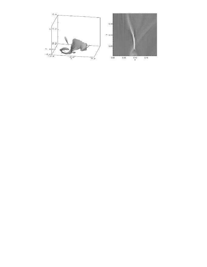
Figure 11.— Vertical current sheet in the unstable configuration at $t=6.6\tau_{\mathrm{A}}$. (Left): Isosurface of current density at $0.1\max(|\bm{j}|)$. (Right): Force-free parameter $\alpha(s,z)$ and in-plane velocity vectors in the vertical cut plane shown in Figure 3. $\alpha=0$ is plotted in gray, and the peak value (white) is $\max(\alpha)=483$ at $(s,z)=(0.092,0.096)$.

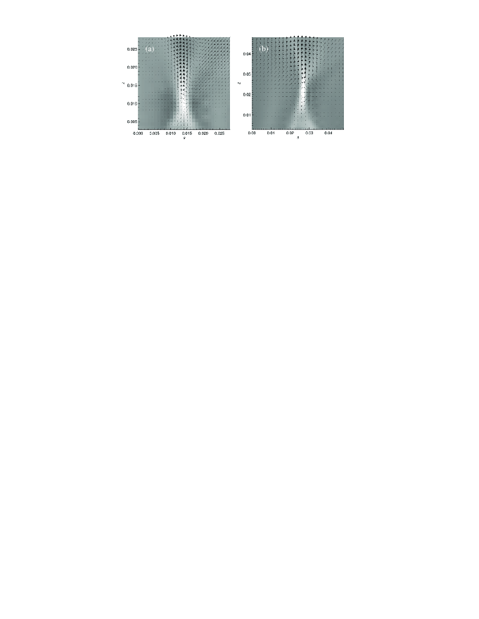
Figure 12.— Reconnection flows of the models with (a) $\Phi_{\mathrm{axi}}=5\times 10^{20}$ Mx and (b) $\Phi_{\mathrm{axi}}=6\times 10^{20}$ Mx in the vertical cut plane shown in Figure 3 at $t=2\tau_{\mathrm{A}}$. The peak in-plane velocities are 0.0045 in (a) and 0.034 in (b). Additionally, $\alpha(s,z)$ is displayed as in Figure 11, with $\max(\alpha)=330$ at $(s,z)=(0.014,0.010)$ in (a) and $\max(\alpha)=404$ at $(s,z)=(0.027,0.023)$ in (b).

The eruption of the rope lifts the overlying flux. This flux is initially sheared (Figure 10) but becomes more antiparallel in the volume under the rope as it is lifted. The corresponding induced current points primarily horizontally and is associated with a Lorentz force pointing toward the essentially vertical layer under the flux rope where the vertical field component of the ambient flux changes sign. The induced current thus pinches into the vertical current sheet, or flare current sheet, known from the standard flare model. One can understand this pinching also as the 3D generalization of the well-known instability of a magnetic X point in two dimensions. The generalized X-type structure is known as an HFT. Its pinching into a current sheet following an appropriate perturbation has been demonstrated by Titov et al. (2003) and Galsgaard et al. (2003). The initial configuration contains such a structure (see Figure 3 and Paper I). Note that the pinching is solely driven by the Lorentz force in our zero-beta simulation (the pressure gradient would additionally contribute if $\beta>0$).

Figure 11 displays the vertical current sheet that forms under the rising flux rope. Since it is a true current sheet (with exponentially rising current density and correspondingly decreasing width in ideal MHD; Titov et al., 2003), the pinching process reaches saturation in a standard one-fluid MHD description only if sufficient diffusion is provided. Otherwise, it proceeds toward the limit of the employed numerical scheme, resulting in unphysical filamentation of the current sheet (which develops on the grid scale and is not related to the plasmoid instability of current sheets; Leboeuf et al., 1982; Loureiro et al., 2007). To verify the eruption of the third model under uniform numerical settings, and as a reference, we have first followed the latter evolution in a run without magnetic field smoothing, $\sigma_{B}=0$. Magnetic reconnection develops in the vertical current sheet and forms coherent reconnection outflows in spite of the ensuing filamentation, so the main ingredients of an eruption—loss of equilibrium and magnetic reconnection—are present in spite of the numerical artefacts. Repeating this run with magnetic field smoothing, chosen to be uniform in the first instance, we find that the flux rope rise velocity is not strongly influenced as long as $\sigma_{B}\lesssim 10^{-3.5}$; it then stays within 20% of its value for $\sigma_{B}=0$. Beyond that level, the rise velocity falls off quickly, and for $\sigma_{B}\geq 10^{-2.5}$ all velocities diffuse away after the initial upward displacement of the rope. It is clear that when the magnetic diffusion $\sigma_{B}$ is large, the currents and Lorentz forces in the body of the flux rope are weaker, artificially stabilizing the solution. The filamentation of the current sheet decreases with increasing $\sigma_{B}$ but disappears only for $\sigma_{B}\gtrsim 10^{-3}$. Therefore, the appropriate numerical setting for the present model consists in applying the smoothing of the magnetic field only in the volume under the flux rope using a level of $\sigma_{B}=10^{-3}$, with a gradual transition to $\sigma_{B}=0$ at the bottom and at the sides. This avoids the filamentation of the vertical current sheet and yields a rise velocity of the flux rope apex very close to (slightly higher than) the value obtained in the absence of the smoothing. Figures 10–16 show the results of this run.

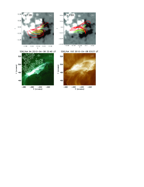
Figure 13.— Reconnected field lines in the unstable configuration in (a) vertical view and (b) perspective view inclined by $25^{\circ}$, overplotted on the magnetogram $B_{z}(x,y,0,t)$. (c–d) Flare loops of the event at the times corresponding to, respectively, $t=2.8\tau_{\mathrm{A}}$ and $t=7.9\tau_{\mathrm{A}}$ in the simulation. Contours of the LOS field component are included in (c). (A color version of this figure is available in the online journal.)

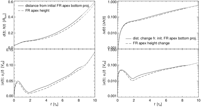
Figure 14.— Rise profile of the flux rope apex in the unstable configuration, shown in the left panels in a format similar to Figure 6. The right panels show the same information on a logarithmic scale. The section of the rise after reflection at the side boundary is plotted in gray.

In addition to the pinching of the HFT under the rising flux rope, part of the current layer at the periphery of the rope steepens, while the main part of the current layer weakens (since the total current through the rope must decrease to power the eruption). The bottom part of the current layer at the side of the flux rope facing the stronger ambient field northeastward of the PIL builds up current densities comparable to the ones in the pinched HFT underneath; thus, the vertical current sheet extends upwards asymmetrically along this side of the flux rope.

The flows triggered by the eruption are shown in the second panel of Figure 11. One can see the rise and expansion velocity in the whole cross section of the flux rope, as well as in the ambient volume, which is threaded by field lines lifted by the rope. The southward inclination of the eruption is apparent. Reconnection flows develop in the vertical current sheet essentially simultaneous with the rise of the rope. The first indication of the downward reconnection outflow becomes visible at $t\approx 1\tau_{\mathrm{A}}$, i.e., already in the initial upward displacement to the rope’s equilibrium height. As the eruption progresses, the reconnection flows evolve joint with the vertical current sheet; thus, they become aligned with the northeastward periphery of the rope in the main phase of the eruption shown in the figure. This asymmetry may contribute to the inclination of the rise direction (consistent with the findings of Panasenco et al., 2011). It may also yield a contribution to the roll effect (Panasenco et al., 2011; Su & van Ballegooijen, 2013), which is weakly indicated by animated field line plots from this simulation, as well as in the EUVI-A data shown below in Figure 15. Finally, we note that the upward reconnection outflow reaches slightly higher velocities than the flux rope and its immediate surroundings, so that the new flux carried into the rope is likely to have a direct positive effect on the acceleration in the main body of the rope.

It is worth noting that the stable model with $\Phi_{\mathrm{axi}}=5\times 10^{20}$ Mx also possesses an HFT (see Figure 3(c) above and Figure 7(d) in Paper I). This HFT pinches as well into a short vertical current sheet during the initial upward displacement, and reconnection commences as early as for the unstable model; see the direct comparison of the models at $t=2\tau_{\mathrm{A}}$ (i.e., after the initial displacement) in Figure 12. However, an eruption does nevertheless not occur. This indicates that reconnection in the vertical current sheet of the considered coronal NLFFF models is not able to drive an eruption by itself, but rather that the driving by an unstable flux rope is required. A downward return flow is induced in the stable case by the rapid initial rise of the flux rope (Figure 12(a)); this would not occur in a quasi-static evolution. This flow is seen to join the reconnection inflow, so it does not appear to work against the further development of reconnection in this model.

Figure 13 compares flare loops and reconnected field lines in the simulation. The selected observation times correspond to $t=2.8\tau_{\mathrm{A}}$ and $t=7.9\tau_{\mathrm{A}}$ in the simulation if the scaling of Section 6.1 is adopted. A similar comparison with field lines of the corresponding MFR model is given in Figure 12 of Paper I. The two sets of green and red field lines are traced from start points at $z=0$ in the positive polarity which lie slightly inside the current layer that extends from the bottom tip of the vertical current sheet at 2.8 and $7.9\tau_{\mathrm{A}}$, so that they are to be compared with the flare loops in panels (c) and (d), respectively. (In the figure, both sets are traced in the field at $7.9\tau_{\mathrm{A}}$; the lower set is visually nearly indistinguishable from the field lines traced in the field at $2.8\tau_{\mathrm{A}}$.) The trend of progressively decreasing shear is very clear in the simulation data as well, see the vertical view in panel (a). The perspective view at an inclination of $25^{\circ}$ from vertical in panel (b) is chosen to correspond to the latitude of $\approx 25^{\circ}$ of the active region (the weak tilt corresponding to the slightly eastward longitude is not taken into account). Here the field line shapes appear basically similar to the shapes of the flare loops. The loops possess slightly higher shear. This is not unexpected, since the use of the potential field in constructing the NLFFF models is likely to remove some of the shear that has accumulated in the ambient field in the earlier evolution of the AR. Part of this shear is recovered in the MFR phase, and the remaining difference appears to be minor for the considered region.

A more significant and expected difference is revealed by the distance of the flare ribbons to the PIL. Compared to the end points of the newly reconnected field lines at $7.9\tau_{\mathrm{A}}$, the separation of the flare ribbons at 03:23 UT is larger by a factor $\approx 1.5$, which signifies a corresponding difference in the reconnection rate. Given that no attempt was made to correctly model the reconnection rate (beyond the choice of the numerical diffusion such that the current sheet does not develop numerical artefacts), the difference is surprisingly small. We expect that it can be removed by including resistivity.

The rise profile of the eruption is plotted in Figure 14. Here the initial, mainly upward-directed displacement leads to a doubling of the initial apex height (from $h_{0}=0.047$ to $h(2)=0.098$) within a time frame similar to the relaxation runs. The flux rope has roughly semicircular shape at this time. As soon as the initial velocity enhancement has largely decayed, one can see a more gradually developing rise with a significant horizontal component (obvious from the increasing difference between the solid and dashed curves in the figure). The logarithmic display reveals that the more gradual rise is approximately exponential (but it can also be approximated by a power law with an exponent near 3). The different functional form and direction of the rise after $t=2\tau_{\mathrm{A}}$ suggest that the two phases have different physical origins. This is supported by the evolution of $\sigma_{j}(t)$, which first decreases monotonically to $\sigma_{j}(t\!=\!3.1)=0.038$ and subsequently increases monotically. We interpret the initial upward displacement as the motion to the equilibrium position of the flux rope which it had not yet reached after the 30,000 MFR iterations that define the initial condition for the MHD run. The subsequent exponential-to-power law rise is characteristic of an instability launched by a small-to-moderate perturbation (Schrijver et al., 2008b) from the obviously unstable equilibrium position.

The fluid element at the magnetic axis of the flux rope experiences the reflection at the side boundary of the box after $t\approx 8\tau_{\mathrm{A}}$. 8.7 (39) percent of the initial total (free) magnetic energy are released at this stage. The subsequent part of the rise profile is not related to reality and included only for completeness. The additional upward acceleration in the process of the reflection results from the induction of currents as the expanding flux is compressed at the side boundary.

6.1. Scaling the Simulation to the Observations

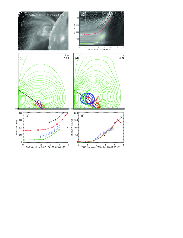
Figure 15.— Scaling of the simulation to the observation data. (a): A representative EUVI-A 195 Å radial-filter image showing the structure of the overlying flux. The indicated artificial slit is aligned with the main expansion direction of $45^{\circ}$ from vertical and used to generate the stack plot in panel (b). (c–d): Field line plots during the nearly exponential rise phase, viewed in $-x$ direction. The field line used for the scaling is marked in blue. (e–f): Scaling of simulation data (blue diamonds and plus signs) to the rise profiles marked in the stack plot. (A color version of this figure and an animation of the EUVI-A 195 Å image sequence are available in the online journal.)

From the rise profile in Figure 14 it is obvious that the simulation can capture properties of the eruption on 2010 April 8 in the early, approximately exponential phase, $2\lesssim t/\tau_{\mathrm{A}}<8$. The quantitative comparison between this part of the rise profile and EUVI-A 195 Å data allows us to scale the simulation to the observed event. Since the erupting flux propagates mainly southwards (as seen in the AIA images), STEREO Ahead observes its rise nearly exactly from the side, presumably with relatively small projection effects. Note that only the scaling of the time unit $\tau_{\mathrm{A}}$, or equivalently of the velocity unit $\hat{V}_{\mathrm{A0}}$, is to be determined, since the length and field strength units are given by the magnetogram and the density is fixed by field strength and Alfvén velocity.

An animation of the EUVI-A 195 Å images is included with Figure 15, and panel (a) shows a representative image. No trace of the rising filament material can be seen, but several overlying loops stand out relatively clearly. Their rise is quantified in the stack plot (panel (b)) taken at an artificial slit which is aligned with the average direction of ascent (see panel (a)). The three clearest traces are marked in color.

Next, we select field lines which correspond to the overlying loops. It turns out that no exact match is possible, since the usable height range in the simulation falls between the lower two traces in the stack plot. This is seen in Figures 15(c) and (d), where a ray is indicated, corresponding to the artificial slit in the EUVI-A image. The panels display a view in $-x$ direction, similar to the view of STEREO Ahead. The ray starts at the apex of the flux rope’s magnetic axis at $t=0$ and lies in the $y$-$z$ plane, inclined to the vertical by $45^{\circ}$. After the initial upward displacement, the flux rope radius has grown such that the innermost overlying flux lies at a distance of about 70 Mm along the ray, larger than the pre-eruption distance of $\approx 40$ Mm of the green trace in the stack plot. The pre-eruption distance of the red trace is about 175 Mm, already relatively close to the side boundary of the box. Flux in this height range can be followed until the compression zone near the side boundary is encountered, roughly at 250 Mm along the ray, but this is, of course, stronger influenced by the side boundary than the flux immediately surrounding the rope, and it can only utilize a small part of the red trace in the stack plot. Nevertheless, using a field line in the innermost overlying flux permits an acceptable scaling, since the expansion of the overlying flux is rather uniform: the three traces run approximately parallel to each other, i.e., with similar velocity profiles.

We thus select a fluid element on the ray which lies slightly outside the flux rope at $t\approx 1.75\tau_{\mathrm{A}}$, the beginning of nearly exponential rise. The trajectory of this fluid element is computed through the simulation. At later times, a field line is traced from the new position and projected onto the $y$-$z$ plane, where its crossing with the ray yields a new projected distance along the ray. Finite differencing yields a projected velocity along the main direction of propagation for both observation and simulation data.

The EUVI-A images (of 2.5 min cadence) place the onset time of the expansion in a relatively narrow interval, 02:30:30–02:33:00 UT, of which we associate a time near the midpoint, 02:32 UT, with $t=1.75\tau_{\mathrm{A}}$ in the simulation. The value $\hat{V}_{\mathrm{A0}}\approx 1400$ km s^-1 that yields a good match of both the projected distance and velocity data is then easily found by trial and error; see the diamonds in Figures 15(e) and (f), which cover the interval $t=(1.73\mbox{--}5.93)\tau_{\mathrm{A}}$ in the simulation. A change of $\pm 100$ km s^-1 from the estimated $\hat{V}_{\mathrm{A0}}$ already produces a much poorer match.

We note that a trend of decreasing acceleration becomes visible in the projected velocity data of the overlying flux in the simulation already in the middle of the considered interval. This is not seen in the observation data and indicates how early the overlying flux is influenced by the side boundary. Nevertheless, the match between simulation and observation appears acceptable up to the second-to-last velocity point in the interval.

An ambiguity in the above procedure originates from the insufficient knowledge about the position of the overlying loops relative to the plane of sky for STEREO Ahead. They cannot be unambiguously identified in the corresponding AIA 193 Å images. We know from AIA that the main direction of expansion was nearly southward, i.e., nearly in the plane of sky for STEREO Ahead, but that the initial expansion had a strong southeastward component. To roughly estimate how this ambiguity might influence the scaling, we repeat the procedure, positioning the fluid element at $t\approx 1.75\tau_{\mathrm{A}}$ on rays directed $\pm 30^{\circ}$ off the meridional plane (but also starting at the flux rope apex). For the southeastward pointing ray, the same $\hat{V}_{\mathrm{A0}}$ is obtained from a match of nearly the same quality (see the plus signs in Figures 15(e) and (f)). For the southwestward pointing ray, a higher Alfvén velocity is indicated (by $\sim 50\%$), but it is not possible to match both distances and velocities to the stack plot data at a reasonable quality. The AIA data do not show any distinctive structure propagating in this direction in the time interval used in the scaling. Thus, we consider it very unlikely that the structures seen by EUVI-A have expanded in this direction. On the other hand, the consistency of the $\hat{V}_{\mathrm{A0}}$ estimates, based on the southward and southeastward directed rays, makes them rather reliable. For completeness we note that the considered fluid elements remain relatively close to their respective ray in the course of the eruption.

The estimated value of the peak initial Alfvén velocity $\hat{V}_{\mathrm{A0}}$ refers to the point of peak field strength in the box, $\max(B_{0})=955$ Gauss, which lies in the magnetogram plane. Our model for the initial density implies $V_{\mathrm{A0}}\propto{B_{0}^{1/4}}$, so that the initial field strength of $\approx 70$ Gauss in the area of the flux rope apex yields an initial Alfvén velocity $V_{\mathrm{A0}}\approx 730$ km s^-1 and initial particle density $N_{0}\approx 4.4\times 10^{10}$ cm^-3 in the upper part of the flux rope. The density must be taken as a characteristic average density in the filament channel, since our density model disregards any filamentary fine structure of the plasma.

One has to consider this velocity as the lower end point of a plausible range (and the density, correspondingly, as an upper end point). This value follows from a model with a certain amount of prescribed axial flux, $\Phi_{\mathrm{axi}}=6\times 10^{20}$ Mx, which lies near the point of marginal stability, but at a somewhat arbitrary distance set by the interval of $10^{20}$ Mx between the $\Phi_{\mathrm{axi}}$ values in consecutive models. An unstable model with less axial flux would yield a slower rise in the simulation, consequently, a higher estimate for $\hat{V}_{\mathrm{A0}}$. Indeed, the leading-edge CME velocity of $\approx 520$ km s^-1 observed by COR2 is at 70% of the Alfvén velocity in the source. Allowing for a factor 2 lower velocity of the CME core, this becomes ${\sim}\,V_{\mathrm{A0}}/3$, still a rather high value for a moderate CME that gains its acceleration in a large height range of several $R_{\odot}$. Such eruptions tend to reach lower terminal flux rope velocities of $\lesssim 0.2V_{\mathrm{A0}}$ (Török & Kliem, 2007). Thus, a range for the Alfvén velocity in the flux rope from $\approx 730$ km s^-1 up to about a factor 2 higher appears reasonable. The corresponding density range is $\sim(1\mbox{--}4)\times 10^{10}$ cm^-3.

These estimates lie well within acceptable ranges. Gary (2001) finds $\beta\sim 0.02\mbox{--}0.2$ at a height of $0.1~{}R_{\odot}$ (see his Figure 3), which translates to $V_{\mathrm{A}}=2C_{\mathrm{s}}\beta^{-1/2}\sim(650\mbox{--}2000)$ km s^-1 for a plasma temperature of $T=2.5$ MK (i.e., a sound speed of $C_{\mathrm{s}}=145$ km s^-1). The lower part of the range is appropriate for a considerably dispersed, moderate AR like AR 11060. Labrosse et al. (2010, their Section 3.3.2) quote the wide range of $N\sim(10^{9}\mbox{--}10^{11})$ cm^-3 for densities of cool (H$\alpha$-emitting) to moderately hot (EUV-emitting) plasmas in quiescent and AR prominences. The lower-to-middle part of the range may be representative for the average density in the erupting flux in the considerably dispersed AR.

6.2. Onset Condition

By reaching good agreement with key features of the eruptive event on 2010 April 8, like the initial height-time profile and the rise direction of the erupting flux, our simulations substantiate the conclusion in Paper I that the flux rope insertion method allows to model the NLFFF in AR 11060 around the time of the eruption. The condition for the loss of equilibrium, formulated as a condition of flux imbalance in terms of the ratio between the rope’s axial flux and the unsigned flux in the source region of the eruption, is also confirmed. Given the total unsigned flux in AR 11060 of $F_{\mathrm{u}}=3.7\times 10^{21}$ Mx (Paper I), the range of $\Phi_{\mathrm{axi}}=(5\mbox{--}6)\times 10^{20}$ Mx for the marginal stability point yields a flux ratio $\Phi_{\mathrm{axi}}/(F_{\mathrm{u}}/2)=(27\mbox{--}32)\%$, well within the range found previously (Bobra et al., 2008; Savcheva et al., 2012b). A similar flux ratio is reached at the onset of eruption in the simulation that applied flux cancellation to the model with $\Phi_{\mathrm{axi}}=5\times 10^{20}$ Mx.

It is of principal interest to compare this condition with the condition obtained by describing the loss of equilibrium as a plasma instability, i.e., the kink instability of a current channel. The relevant mode of the kink instability here is the lateral kink, known as the torus instability in the case of an arched current channel, since the pre-eruptive NLFFF possesses insufficient twist for the excitation of the helical kink mode. Using the length and flux values of the two flux rope models next to the marginally stable point, $L\approx 270$ Mm, $\Phi_{\mathrm{axi}}=(5\mbox{--}6)\times 10^{20}$ Mx, and $F_{\mathrm{pol}}=10^{10}$ Mx cm^-1, the average twist angle is $LB_{\phi}/(rB_{z})\sim{\pi}LF_{\mathrm{pol}}/\Phi_{\mathrm{axi}}=(0.53\mbox{--}0.45)\pi$, far smaller than the threshold of the helical kink.

The threshold of the torus instability is given in terms of the decay index of the external poloidal field, $B_{\mathrm{ep}}$, at the position of the current channel, $n=-d\ln{B_{\mathrm{ep}}}/d\ln{z}>n_{\mathrm{cr}}$. The canonical values of the critical decay index are $n_{\mathrm{cr}}=3/2$ for a toroidal current channel (Bateman, 1978) and $n_{\mathrm{cr}}=1$ for a straight current channel (van Tend & Kuperus, 1978). Kliem & Török (2006) showed that the value for a toroidal current channel rises to $n_{\mathrm{cr}}=2$ if reconnection under the flux rope does not commence immediately, and they added a relatively small negative correction term. Démoulin & Aulanier (2010) generalized the consideration to arbitrarily shaped paths of the current channel, finding a range $n_{\mathrm{cr}}\approx 1.1\mbox{--}1.3$. Most numerical studies, including the only parametric study to date, find $n_{\mathrm{cr}}$ in the range 1.5–1.75 (Török & Kliem, 2007; Aulanier et al., 2010; Fan, 2010), but it should be noted that the simulation in Fan & Gibson (2007) yields a value of 1.9. The range 1.5–1.75 is also supported by observational studies (Liu, 2008; Guo et al., 2010). The critical decay index must depend upon the photospheric line tying (which varies with the shape of the current channel) and it should increase for increasing strength of the external toroidal (shear) field. These dependencies have not yet been investigated. However, we can expect these effects to be relatively minor in the present case, since the line tying is minimized for semicircular flux rope shape, which the unstable flux rope reaches at the onset of the eruption, and since the ambient potential field has only little shear. In the comparison below, we adopt the currently best supported range of the torus instability threshold, $n_{\mathrm{cr}}\approx 1.5\mbox{--}1.75$.

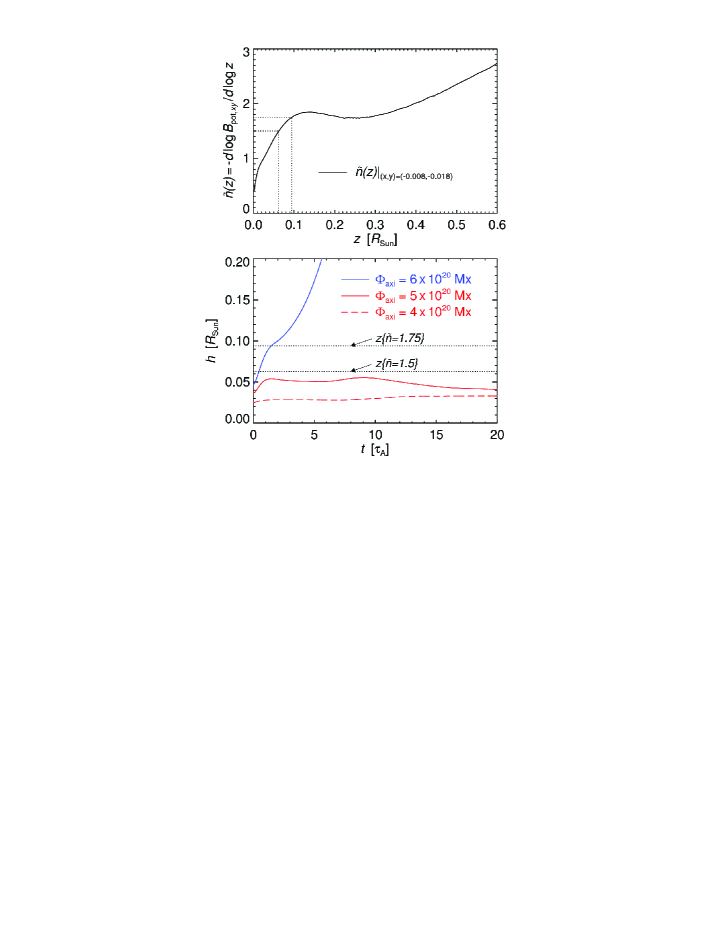
Figure 16.— (a) Decay index $\tilde{n}=-d\ln{B_{\mathrm{pot,\,\textit{xy}}}}/d\ln{h}$ of the horizontal components of the potential field along a vertical line passing through the apex point of the flux rope’s magnetic axis at $t=0$. (b) Height-time profiles of the flux rope apex for the three models studied in this paper, compared to the onset condition of the torus instability. (A color version of this figure is available in the online journal.)

In practice it is often impossible or rather laborious to isolate the external poloidal field $B_{\mathrm{ep}}$. This involves the subtraction of the poloidal field created by the current channel in the corona, which requires the exact knowledge of the current channel, i.e. of the NLFFF. Here we have this knowledge from the relaxed configuration with $\Phi_{\mathrm{axi}}=5\times 10^{20}$ Mx and from the initial configuration with $\Phi_{\mathrm{axi}}=6\times 10^{20}$ Mx. However, given the effort required for this analysis and given the uncertainty in the knowledge of the critical decay index, we choose to simplify the consideration by instead using the decay index of the horizontal component of the (total) potential field, $\tilde{n}=-d\ln{B_{\mathrm{pot,\,\textit{xy}}}}/d\ln{z}$. We have verified that the potential field passes at nearly right angles over the PIL in the height range of the flux rope at $t=0$, so that it is a reasonable approximation of the external poloidal field. The direction is much closer to perpendicular than that of the immediately overlying flux in the initial configuration of the MHD simulation (green field lines in Figure 10 at $t=0$), which is considerably influenced by the presence of the flux rope in the course of the MFR. We have computed $\tilde{n}(z)$ at several positions along the PIL and found it to be nearly uniform in the section of the PIL between the main flux concentrations where the middle part of the inserted flux rope is located. Figure 16 shows the profile at the vertical line through the flux rope apex. The height range corresponding to the adopted range of $n_{\mathrm{cr}}$ is $z=0.063\mbox{--}0.094$.

The bottom panel of Figure 16 summarizes the height-time profiles of the three models studied in this paper. The apex of two stable ones stays in the range $h\approx 0.03\mbox{--}0.055$, i.e. below the torus-unstable height range. The inferred equilibrium apex height of the unstable model, $h(t\!=\!2)=0.098$, falls rather clearly in the torus-unstable height range (as discussed above, the rise up to the equilibrium height is not related to an instability). Thus, for the considered AR 11060, the stability boundary given in terms of the axial flux in the rope, $\Phi_{\mathrm{axi}}=(5\mbox{--}6)\times 10^{20}$ Mx, corresponds very well to the most likely range for the threshold of the torus instability, $n_{\mathrm{cr}}\approx 1.5\mbox{--}1.75$.

7. Summary and Conclusions

This paper reports MHD simulations that study NLFFF models of the eruptive AR 11060. The models were constructed in Paper I (Su et al., 2011) using the flux rope insertion method and MFR. We selected three that appeared to best represent the pre-eruptive, nearly marginally stable, and eruptive states of the active region, differing only in the axial flux of the inserted flux rope, which encompasses the range $\Phi_{\mathrm{axi}}=(4\mbox{--}6)\times 10^{20}$ Mx. Our simulations confirm key results of Paper I:

1. There is a limiting value of the axial flux in the rope for the existence of stable NLFFF equilibria, which lies in the selected range. The equilibrium height of the flux rope increases with axial flux.

2. Stable models relax deeply in the MHD simulation, reaching numerical equilibria that retain a flux rope in the considered range of $\Phi_{\mathrm{axi}}$. Field lines in the flux rope and its immediate surrounding correspond well in shape to the observed coronal loops.

3. The flux rope in the unstable model experiences a full eruption.

Thus, although none of the observed structures in AR 11060 shows regular multiple crossings, the definite signature of a flux rope, our simulations substantiate the conclusions in Paper I that a flux rope existed in the active region prior to the eruption and that the rope’s loss of equilibrium caused the eruption. Additionally, we obtain the following results:

1. The model with $\Phi_{\mathrm{axi}}=5\times 10^{20}$ Mx, found to be nearly marginally stable in Paper I, is also found to be closest to marginal stability—on the stable side. It does not erupt even though the HFT at its underside pinches into a short vertical current sheet and a transient phase of reconnection in this current sheet is triggered, lasting for a couple of Alfvén times. The model can be driven to eruption by photospheric flux cancellation, and the ratio of its axial and unsigned flux at that point is similar to the flux ratio of the unstable model.

2. The erupting flux rope shows an accelerated rise $h(t)$, which can be approximated by an exponential and also by a power-law with an index near 3. Such a rise is characteristic of a flux rope instability (Schrijver et al., 2008b). The rise velocity reaches a considerable fraction of the initial Alfvén velocity in the flux rope, about 20% (still rising when the boundary of the simulation box is approached). This indicates that the model lies clearly in the unstable domain of parameter space.

3. The simulated eruption agrees very well with several characteristics of the modeled event, including (i) the initially very inclined direction of ascent, by $45^{\circ}$ from vertical toward the equator; (ii) the accelerated rise of the overlying flux; and (iii) the close temporal association between the acceleration of the flux rope (the CME component of the eruption) and the development of reconnection in the vertical current sheet underneath (the flare component). Additionally, initially high shear and the trend of progressively decreasing shear in the reconnected flux under the rope, as displayed by the flare loops, are clearly reproduced. However, there are also differences. (i) The simulated rise begins to turn more radial in the low corona, whereas the modeled event showed an increasing inclination in the low corona, turning more radial only at heights of several solar radii. (ii) The footpoint locations of newly reconnected field lines in the simulation move away from the PIL at a somewhat lower speed than the observed flare ribbons, indicating a moderately lower reconnection rate. Obvious reasons and straightforward options for improvement of the modeling were identified for both.

4. Oblique eruption paths can be caused by the specifics of the magnetic structure in the source region, in addition to the interaction with a coronal hole and the asymmetry of the photospheric flux distribution suggested earlier (Gopalswamy et al., 2009; Panasenco et al., 2013). We suggest that the slingshot action of horizontally curved flux, which was, or quickly became, part of the erupting flux, contributed to the inclination of the rise path in the modeled event.

5. The ability to follow the eruption allows us to scale the simulation to the observation data, thus estimating the Alfvén velocity in the source region of the eruption. The range $V_{A}\sim(730\mbox{--}1500)$ km s^-1 in the volume of the flux rope is indicated. Since the field strength in the rope is given by the NLFFF model, $B\approx 70$ Gauss, the estimated Alfvén velocity implies an average flux rope density in the range $N\sim(1\mbox{--}4)\times 10^{10}$ cm^-3. Both values lie within acceptable ranges, especially the Alfvén velocity, since AR 11060 was already considerably dispersed.

6. By its sharper discrimination between stability and instability compared to the magnetofrictional relaxation technique, the MHD modeling yields a narrower range for the threshold value of the considered control parameter. We find that the value lies in the range $\Phi_{\mathrm{axi}}=(5\mbox{--}6)\times 10^{20}$ Mx (compared to $(4\mbox{--}6)\times 10^{20}$ Mx in Paper I). This corresponds to a range of the flux ratio $\Phi_{\mathrm{axi}}/(F_{\mathrm{u}}/2)=0.27\mbox{--}0.32$, where $F_{\mathrm{u}}=3.7\times 10^{21}$ Mx is the total unsigned flux in the AR.

7. This range of the flux ratio corresponds very well to the threshold of the torus instability in the considered active region. Using the horizontal component of the potential field as a proxy for the external poloidal field component, the decay index $n=-d\ln{B_{\mathrm{ep}}}/d\ln{z}$ takes values $n\approx 1.3\mbox{--}1.8$ in the range of equilibrium flux rope heights found for the range of axial flux $\Phi_{\mathrm{axi}}=(5\mbox{--}6)\times 10^{20}$ Mx. The critical decay index for onset of the torus instability is estimated to lie in the range $n_{\mathrm{cr}}\approx 1.5\mbox{--}1.75$. This establishes a connection between these independently developed criteria for the loss of equilibrium of a flux rope, which is plausible from the following consideration. Higher axial flux in the rope corresponds to greater equilibrium height (as a consequence of the implied higher flux rope current), which, in turn, typically corresponds to higher decay index, i.e., to approaching the torus-unstable height range where $n>n_{\mathrm{cr}}$.

8. A considerable amount of changes were found while the stable models relaxed to a numerical equilibrium in the MHD simulation, although they had already gone through an MFR phase. The MFR had a pre-set number of iterations, thus it had not progressed to the deepest level possible, especially not for the nearly marginally stable model, but the model with $\Phi_{\mathrm{axi}}=4\times 10^{20}$ Mx was quite well relaxed. Even changes of the topology (a transient split of the flux rope) occurred in the MHD relaxation. Only a part of the different level of dynamics appears to be due to the numerical differences between the employed magnetofrictional and MHD simulation codes. A systematic comparison of magnetofrictional vs. MHD relaxation might thus be warranted.

Based on various developments and applications of the flux rope insertion method (e.g., van Ballegooijen, 2004; Bobra et al., 2008; Su et al., 2011), this research represents a further step toward data-constrained numerical modeling of solar eruptions. Future work along this line will consider coronal NLFFF constructed from a time series of magnetograms, as in Savcheva & van Ballegooijen (2009) and Savcheva et al. (2012b), and eventually proceed to driving coronal NLFFF through time-dependent photospheric boundary data obtained from observations. Technical improvements toward using larger domains and open boundary conditions will permit following eruptions much further than possible here; this will set tighter constrains as well.

References

- Amari et al. (2011) Amari, T., Aly, J.-J., Luciani, J.-F., Mikic, Z., & Linker, J. 2011, ApJ, 742, L27
- Amari et al. (2010) Amari, T., Aly, J.-J., Mikic, Z., & Linker, J. 2010, ApJ, 717, L26
- Aulanier et al. (2010) Aulanier, G., Török, T., Démoulin, P., & DeLuca, E. E. 2010, ApJ, 708, 314
- Bateman (1978) Bateman, G. 1978, MHD instabilities (MIT Press, Cambridge, MA)
- Bobra et al. (2008) Bobra, M. G., van Ballegooijen, A. A., & DeLuca, E. E. 2008, ApJ, 672, 1209
- Canou & Amari (2010) Canou, A., & Amari, T. 2010, ApJ, 715, 1566
- De Rosa et al. (2009) De Rosa, M. L., Schrijver, C. J., Barnes, G., Leka, K. D., Lites, B. W., Aschwanden, M. J., Amari, T., Canou, A., McTiernan, J. M., Régnier, S., Thalmann, J. K., Valori, G., Wheatland, M. S., Wiegelmann, T., Cheung, M. C. M., Conlon, P. A., Fuhrmann, M., Inhester, B., & Tadesse, T. 2009, ApJ, 696, 1780
- Démoulin & Aulanier (2010) Démoulin, P., & Aulanier, G. 2010, ApJ, 718, 1388
- Fan (2010) Fan, Y. 2010, ApJ, 719, 728
- Fan & Gibson (2007) Fan, Y., & Gibson, S. E. 2007, ApJ, 668, 1232
- Forbes (2000) Forbes, T. G. 2000, J. Geophys. Res., 105, 23153
- Galsgaard et al. (2003) Galsgaard, K., Titov, V. S., & Neukirch, T. 2003, ApJ, 595, 506
- Gary (2001) Gary, G. A. 2001, Sol. Phys., 203, 71
- Golub et al. (2007) Golub, L., Deluca, E., Austin, G., Bookbinder, J., Caldwell, D., Cheimets, P., Cirtain, J., Cosmo, M., Reid, P., Sette, A., Weber, M., Sakao, T., Kano, R., Shibasaki, K., Hara, H., Tsuneta, S., Kumagai, K., Tamura, T., Shimojo, M., McCracken, J., Carpenter, J., Haight, H., Siler, R., Wright, E., Tucker, J., Rutledge, H., Barbera, M., Peres, G., & Varisco, S. 2007, Sol. Phys., 243, 63
- Gopalswamy et al. (2009) Gopalswamy, N., Mäkelä, P., Xie, H., Akiyama, S., & Yashiro, S. 2009, J. Geophys. Res., 114, A00A22
- Guo et al. (2010) Guo, Y., Ding, M. D., Schmieder, B., Li, H., Török, T., & Wiegelmann, T. 2010, ApJ, 725, L38
- Howard et al. (2008) Howard, R. A., Moses, J. D., Vourlidas, A., Newmark, J. S., Socker, D. G., Plunkett, S. P., Korendyke, C. M., Cook, J. W., Hurley, A., Davila, J. M., Thompson, W. T., St Cyr, O. C., Mentzell, E., Mehalick, K., Lemen, J. R., Wuelser, J. P., Duncan, D. W., Tarbell, T. D., Wolfson, C. J., Moore, A., Harrison, R. A., Waltham, N. R., Lang, J., Davis, C. J., Eyles, C. J., Mapson-Menard, H., Simnett, G. M., Halain, J. P., Defise, J. M., Mazy, E., Rochus, P., Mercier, R., Ravet, M. F., Delmotte, F., Auchere, F., Delaboudiniere, J. P., Bothmer, V., Deutsch, W., Wang, D., Rich, N., Cooper, S., Stephens, V., Maahs, G., Baugh, R., McMullin, D., & Carter, T. 2008, Space Sci. Rev., 136, 67
- Kliem & Török (2006) Kliem, B., & Török, T. 2006, Phys. Rev. Lett., 96, 255002
- Kliem et al. (2012) Kliem, B., Török, T., & Thompson, W. T. 2012, Sol. Phys., 281, 137
- Kuperus & Raadu (1974) Kuperus, M., & Raadu, M. A. 1974, A&A, 31, 189
- Labrosse et al. (2010) Labrosse, N., Heinzel, P., Vial, J.-C., Kucera, T., Parenti, S., Gunár, S., Schmieder, B., & Kilper, G. 2010, Space Sci. Rev., 151, 243
- Leboeuf et al. (1982) Leboeuf, J. N., Tajima, T., & Dawson, J. M. 1982, Physics of Fluids, 25, 784
- Lemen et al. (2012) Lemen, J. R., Title, A. M., Akin, D. J., Boerner, P. F., Chou, C., Drake, J. F., Duncan, D. W., Edwards, C. G., Friedlaender, F. M., Heyman, G. F., Hurlburt, N. E., Katz, N. L., Kushner, G. D., Levay, M., Lindgren, R. W., Mathur, D. P., McFeaters, E. L., Mitchell, S., Rehse, R. A., Schrijver, C. J., Springer, L. A., Stern, R. A., Tarbell, T. D., Wuelser, J.-P., Wolfson, C. J., Yanari, C., Bookbinder, J. A., Cheimets, P. N., Caldwell, D., Deluca, E. E., Gates, R., Golub, L., Park, S., Podgorski, W. A., Bush, R. I., Scherrer, P. H., Gummin, M. A., Smith, P., Auker, G., Jerram, P., Pool, P., Soufli, R., Windt, D. L., Beardsley, S., Clapp, M., Lang, J., & Waltham, N. 2012, Sol. Phys., 275, 17
- Liu et al. (2010) Liu, W., Nitta, N. V., Schrijver, C. J., Title, A. M., & Tarbell, T. D. 2010, ApJ, 723, L53
- Liu (2008) Liu, Y. 2008, ApJ, 679, L151
- Loureiro et al. (2007) Loureiro, N. F., Schekochihin, A. A., & Cowley, S. C. 2007, Physics of Plasmas, 14, 100703
- Metcalf et al. (2008) Metcalf, T. R., De Rosa, M. L., Schrijver, C. J., Barnes, G., van Ballegooijen, A. A., Wiegelmann, T., Wheatland, M. S., Valori, G., & McTtiernan, J. M. 2008, Sol. Phys., 247, 269
- Nindos et al. (2012) Nindos, A., Patsourakos, S., & Wiegelmann, T. 2012, ApJ, 748, L6
- Ofman & Thompson (2011) Ofman, L., & Thompson, B. J. 2011, ApJ, 734, L11
- Panasenco et al. (2011) Panasenco, O., Martin, S., Joshi, A. D., & Srivastava, N. 2011, Journal of Atmospheric and Solar-Terrestrial Physics, 73, 1129
- Panasenco et al. (2013) Panasenco, O., Martin, S. F., Velli, M., & Vourlidas, A. 2013, Sol. Phys., 287, 391
- Robbrecht et al. (2009) Robbrecht, E., Berghmans, D., & Van der Linden, R. A. M. 2009, ApJ, 691, 1222
- Sato & Hayashi (1979) Sato, T., & Hayashi, T. 1979, Physics of Fluids, 22, 1189
- Savcheva et al. (2012a) Savcheva, A., Pariat, E., van Ballegooijen, A., Aulanier, G., & DeLuca, E. 2012a, ApJ, 750, 15
- Savcheva & van Ballegooijen (2009) Savcheva, A., & van Ballegooijen, A. 2009, ApJ, 703, 1766
- Savcheva et al. (2012b) Savcheva, A. S., Green, L. M., van Ballegooijen, A. A., & DeLuca, E. E. 2012b, ApJ, 759, 105
- Savcheva et al. (2012c) Savcheva, A. S., van Ballegooijen, A. A., & DeLuca, E. E. 2012c, ApJ, 744, 78
- Schou et al. (2012) Schou, J., Scherrer, P. H., Bush, R. I., Wachter, R., Couvidat, S., Rabello-Soares, M. C., Bogart, R. S., Hoeksema, J. T., Liu, Y., Duvall, T. L., Akin, D. J., Allard, B. A., Miles, J. W., Rairden, R., Shine, R. A., Tarbell, T. D., Title, A. M., Wolfson, C. J., Elmore, D. F., Norton, A. A., & Tomczyk, S. 2012, Sol. Phys., 275, 229
- Schrijver et al. (2011) Schrijver, C. J., Aulanier, G., Title, A. M., Pariat, E., & Delannée, C. 2011, ApJ, 738, 167
- Schrijver et al. (2008a) Schrijver, C. J., De Rosa, M. L., Metcalf, T., Barnes, G., Lites, B., Tarbell, T., McTiernan, J., Valori, G., Wiegelmann, T., Wheatland, M. S., Amari, T., Aulanier, G., Démoulin, P., Fuhrmann, M., Kusano, K., Régnier, S., & Thalmann, J. K. 2008a, ApJ, 675, 1637
- Schrijver et al. (2006) Schrijver, C. J., De Rosa, M. L., Metcalf, T. R., Liu, Y., McTiernan, J., Régnier, S., Valori, G., Wheatland, M. S., & Wiegelmann, T. 2006, Sol. Phys., 235, 161
- Schrijver et al. (2008b) Schrijver, C. J., Elmore, C., Kliem, B., Török, T., & Title, A. M. 2008b, ApJ, 674, 586
- Su et al. (2011) Su, Y., Surges, V., van Ballegooijen, A., DeLuca, E., & Golub, L. 2011, ApJ, 734, 53
- Su & van Ballegooijen (2012) Su, Y., & van Ballegooijen, A. 2012, ApJ, 757, 168
- Su & van Ballegooijen (2013) —. 2013, ApJ, 764, 91
- Su et al. (2009) Su, Y., van Ballegooijen, A., Lites, B. W., Deluca, E. E., Golub, L., Grigis, P. C., Huang, G., & Ji, H. 2009, ApJ, 691, 105
- Sun et al. (2012) Sun, X., Hoeksema, J. T., Liu, Y., Wiegelmann, T., Hayashi, K., Chen, Q., & Thalmann, J. 2012, ApJ, 748, 77
- Titov (2007) Titov, V. S. 2007, ApJ, 660, 863
- Titov & Démoulin (1999) Titov, V. S., & Démoulin, P. 1999, A&A, 351, 707
- Titov et al. (2003) Titov, V. S., Galsgaard, K., & Neukirch, T. 2003, ApJ, 582, 1172
- Titov et al. (2002) Titov, V. S., Hornig, G., & Démoulin, P. 2002, J. Geophys. Res., 107, 1164
- Török & Kliem (2003) Török, T., & Kliem, B. 2003, A&A, 406, 1043
- Török & Kliem (2005) —. 2005, ApJ, 630, L97
- Török & Kliem (2007) —. 2007, Astronomische Nachrichten, 328, 743
- Valori et al. (2012) Valori, G., Green, L. M., Démoulin, P., Vargas Domínguez, S., van Driel-Gesztelyi, L., Wallace, A., Baker, D., & Fuhrmann, M. 2012, Sol. Phys., 278, 73
- Valori et al. (2010) Valori, G., Kliem, B., Török, T., & Titov, V. S. 2010, A&A, 519, A44
- van Ballegooijen (2004) van Ballegooijen, A. A. 2004, ApJ, 612, 519
- van Ballegooijen et al. (2007) van Ballegooijen, A. A., Deluca, E. E., Squires, K., & Mackay, D. H. 2007, J. Atmosph. Solar-Terr. Phys., 69, 24
- van Ballegooijen et al. (2000) van Ballegooijen, A. A., Priest, E. R., & Mackay, D. H. 2000, ApJ, 539, 983
- van Tend & Kuperus (1978) van Tend, W., & Kuperus, M. 1978, Sol. Phys., 59, 115
- Vršnak et al. (2002) Vršnak, B., Magdalenić, J., Aurass, H., & Mann, G. 2002, A&A, 396, 673
- Yan et al. (2001) Yan, Y., Deng, Y., Karlický, M., Fu, Q., Wang, S., & Liu, Y. 2001, ApJ, 551, L115
- Yang et al. (1986) Yang, W. H., Sturrock, P. A., & Antiochos, S. K. 1986, ApJ, 309, 383
- Yelles Chaouche et al. (2012) Yelles Chaouche, L., Kuckein, C., Martínez Pillet, V., & Moreno-Insertis, F. 2012, ApJ, 748, 23
- Zharkov et al. (2011) Zharkov, S., Green, L. M., Matthews, S. A., & Zharkova, V. V. 2011, ApJ, 741, L35