Polynomial Time Algorithm for Min-Ranks of Graphs with Simple Tree Structures^†

Abstract

The min-rank of a graph was introduced by Haemers (1978) to bound the Shannon capacity of a graph. This parameter of a graph has recently gained much more attention from the research community after the work of Bar-Yossef et al. (2006). In their paper, it was shown that the min-rank of a graph ${\mathcal{G}}$ characterizes the optimal scalar linear solution of an instance of the Index Coding with Side Information (ICSI) problem described by the graph ${\mathcal{G}}$.

It was shown by Peeters (1996) that computing the min-rank of a general graph is an NP-hard problem. There are very few known families of graphs whose min-ranks can be found in polynomial time. In this work, we introduce a new family of graphs with efficiently computed min-ranks. Specifically, we establish a polynomial time dynamic programming algorithm to compute the min-ranks of graphs having simple tree structures. Intuitively, such graphs are obtained by gluing together, in a tree-like structure, any set of graphs for which the min-ranks can be determined in polynomial time. A polynomial time algorithm to recognize such graphs is also proposed.

1 Introduction

1.1 Background

Building communication schemes which allow participants to communicate efficiently has always been a challenging yet intriguing problem for information theorists. Index Coding with Side Information (ICSI) ([5], [6]) is a communication scheme dealing with broadcast channels in which receivers have prior side information about the messages to be transmitted. Exploiting the knowledge about the side information, the sender may significantly reduce the number of required transmissions compared with the naive approach (see Example 3.3). As a consequence, the efficiency of the communication over this type of broadcast channels could be dramatically improved. Apart from being a special case of the well-known (non-multicast) Network Coding problem ([1], [20]), the ICSI problem has also found various potential applications on its own, such as audio- and video-on-demand, daily newspaper delivery, data pushing, and opportunistic wireless networks ([5], [6], [2], [15], [19], [18]).

In the work of Bar-Yossef et al. [2], the optimal transmission rate of scalar linear index codes for an ICSI instance was neatly characterized by the so-called min-rank of the side information graph corresponding to that instance. The concept of min-rank of a graph was first introduced by Haemers [16], which serves as an upper bound for the celebrated Shannon capacity of a graph [25]. This upper bound, as pointed out by Haemers, although is usually not as good as the Lovász bound [22], is sometimes tighter and easier to compute. However, as shown by Peeters [24], computing the min-rank of a general graph (that is, the Min-Rank problem) is a hard task. More specifically, Peeters showed that deciding whether the min-rank of a graph is smaller than or equal to three is an NP-complete problem. The interest in the Min-Rank problem has grown significantly after the work of Bar-Yossef et al. [2]. Subsequently, Lubetzky and Stav [23] constructed a family of graphs for which the min-rank over the binary field is strictly larger than the min-rank over a nonbinary field. This disproved a conjecture by Bar-Yossef et al. [2] which stated that binary min-rank provides an optimal solution for the ICSI problem. Exact and heuristic algorithms to find min-rank over the binary field of a graph was developed in the work of Chaudhry and Sprintson [8]. The min-rank of a random graph was investigated by Haviv and Langberg [17]. A dynamic programming approach was proposed by Berliner and Langberg [3] to compute in polynomial time min-ranks of outerplanar graphs. Algorithms to approximate min-ranks of graphs with bounded min-ranks were studied by Chlamtac and Haviv [9]. They also pointed out a tight upper bound for the Lovász $\vartheta$-function [22] of graphs in terms of their min-ranks. It is also worth noting that approximating min-ranks of graphs within any constant ratio is known to be NP-hard (see Langberg and Sprintson [21]).

1.2 Our Contribution

So far, families of graphs whose min-ranks are either known or computable in polynomial time are the following: odd cycles and their complements, perfect graphs, and outerplanar graphs. Inspired by the work of Berliner and Langberg [3], we develop a dynamic programming algorithm to compute the min-ranks of graphs having simple tree structures. Loosely speaking, such a graph can be described as a compound rooted tree, the nodes of which are induced subgraphs whose min-ranks can be computed in polynomial time.

Figure 1: A graph ${\mathcal{G}}$ with a simple tree structure

As an illustrative example, a graph ${\mathcal{G}}$ with a simple tree structure is depicted in Figure 1. In this example, each induced subgraph (node) ${\mathcal{G}}_{i}$ ($i\in[9]$) of ${\mathcal{G}}$ is either a perfect graph or an outerplanar graph (hence ${\mathcal{G}}_{i}$’s min-rank can be efficiently computed). The dynamic programming algorithm (Algorithm 1) computes the min-ranks of the subtrees, from the leaves to the root, in a bottom-up manner. The task of computing the min-rank of a graph is accomplished when the computation reaches the root of the compound tree. Let ${\mathscr{F}}_{\mathscr{P}}(c)$, roughly speaking, denote the family of graphs with simple tree structures where each node in the tree structure is connected to its child nodes via at most $c$ vertices. For instance, the graph ${\mathcal{G}}$ depicted in Figure 1 belongs to the family ${\mathscr{F}}_{\mathscr{P}}(2)$. We prove that Algorithm 1 runs in polynomial time if ${\mathcal{G}}\in{\mathscr{F}}_{\mathscr{P}}(c)$, and also provide another algorithm (Algorithm 2) that recognizes a member of ${\mathscr{F}}_{\mathscr{P}}(c)$ in polynomial time, for any constant $c>0$.

In fact, Algorithm 1 still runs in polynomial time for graphs belonging to a larger family ${\mathscr{F}}_{\mathscr{P}}(c\log(\cdot))$. This family consists of graphs ${\mathcal{G}}$ with simple tree structures where each node in the tree structure is connected to its child nodes via at most $c\log|\mathcal{V}(\mathcal{G})|$ vertices. However, finding a polynomial time recognition algorithm for members of ${\mathscr{F}}_{\mathscr{P}}(c\log(\cdot))$ is still an open problem.

Another way to look at our result is as follows. From a given set of graphs ${\mathcal{G}}_{i}$ ($i\in[k]$) whose min-ranks can be computed in polynomial time, one can build a new graph ${\mathcal{G}}$ such that ${\mathcal{G}}_{i}$ ($i\in[k]$) are all the connected components of ${\mathcal{G}}$. Then by Lemma 3.4, the min-rank of ${\mathcal{G}}$ can be trivially computed by taking the sum of all the min-ranks of ${\mathcal{G}}_{i}$ ($i\in[k]$). This is a trivial way to build up a new graph whose min-rank can be efficiently computed from a given set of graphs whose min-ranks can be efficiently computed. Our main contribution is to provide a method to build up in a nontrivial way an infinite family of new graphs with min-ranks computable in polynomial time from given families of graphs with min-ranks computable in polynomial time. This new family can be further enlarged whenever a new family of graphs (closed under induced subgraphs) with min-ranks computable in polynomial time is discovered. Using this method, roughly speaking, from a given set of graphs, we build up a new one by introducing edges that connect these graphs in such a way that a tree structure is formed.

It is also worth mentioning that the min-ranks of all non-isomorphic graphs of order up to $10$ can be found using a computer program that combines a SAT-based approach [8] and a Branch-and-Bound approach.

1.3 Organization

The paper is organized as follows. Basic notation and definitions are presented in Section 2. The ICSI problem is formally formulated in Section 3. The dynamic programming algorithm that computes in polynomial time min-ranks of the graphs with simple tree structures is presented in Section 4. An algorithm that recognizes such graphs in polynomial time is also developed therein. We mention the computation of min-ranks of all non-isomorphic graphs of small orders in Section 5. Finally, some interesting open problems are proposed in Section 6.

2 Notation and Definitions

We use $[n]$ to denote the set of integers $\{1,2,\ldots,n\}$. We also use $\mathbb{F}_{q}$ to denote the finite field of $q$ elements. For an $n\times k$ matrix ${\boldsymbol{M}}$, let ${\boldsymbol{M}}_{i}$ denote the $i$th row of ${\boldsymbol{M}}$. For a set $E\subseteq[n]$, let ${\boldsymbol{M}}_{E}$ denote the $|E|\times k$ sub-matrix of ${\boldsymbol{M}}$ formed by rows of ${\boldsymbol{M}}$ that are indexed by the elements of $E$. For any matrix ${\boldsymbol{M}}$ over $\mathbb{F}_{q}$, we denote by ${\mathsf{rank}_{q}}({\boldsymbol{M}})$ the rank of ${\boldsymbol{M}}$ over $\mathbb{F}_{q}$.

A simple graph is a pair ${\mathcal{G}}=(\mathcal{V}(\mathcal{G}),\mathcal{E}(\mathcal{G}))$ where $\mathcal{V}(\mathcal{G})$ is the set of vertices of ${\mathcal{G}}$ and $\mathcal{E}(\mathcal{G})$ is a set of unordered pairs of distinct vertices of ${\mathcal{G}}$. We refer to $\mathcal{E}(\mathcal{G})$ as the set of edges of ${\mathcal{G}}$. A typical edge of ${\mathcal{G}}$ is of the form $\{u,v\}$ where $u\in\mathcal{V}(\mathcal{G})$, $v\in\mathcal{V}(\mathcal{G})$, and $u\neq v$. If $e=\{u,v\}\in\mathcal{E}(\mathcal{G})$ we say that $u$ and $v$ are adjacent. We also refer to $u$ and $v$ as the endpoints of $e$. We denote by $N^{\mathcal{G}}(u)$ the set of neighbors of $u$, namely, the set of vertices adjacent to $u$.

Simple graphs have no loops and no parallel edges. In the scope of this paper, only simple graphs are considered. Therefore, we use graphs to refer to simple graphs for succinctness. The number of vertices $|\mathcal{V}(\mathcal{G})|$ is called the order of ${\mathcal{G}}$, whereas the number of edges $|\mathcal{E}(\mathcal{G})|$ is called the size of ${\mathcal{G}}$. The complement of a graph ${\mathcal{G}}=(\mathcal{V}(\mathcal{G}),\mathcal{E}(\mathcal{G}))$, denoted by $\overline{{\mathcal{G}}}=(\mathcal{V}(\overline{\mathcal{G}}),\mathcal{E}(\overline{\mathcal{G}}))$, is defined as follows. The vertex set $\mathcal{V}(\overline{\mathcal{G}})=\mathcal{V}(\mathcal{G})$. The arc set

$$\mathcal{E}(\overline{\mathcal{G}})=\big{\{}\{u,v\}:\ u,v\in\mathcal{V}(\mathcal{G}),\ u\neq v,\ \{u,v\}\notin\mathcal{E}(\mathcal{G})\big{\}}.$$

A subgraph of a graph ${\mathcal{G}}$ is a graph whose vertex set $V$ is a subset of that of ${\mathcal{G}}$ and whose edge set is a subset of that of ${\mathcal{G}}$ restricted on the vertices in $V$. The subgraph of ${\mathcal{G}}$ induced by $V\subseteq\mathcal{V}(\mathcal{G})$ is a graph whose vertex set is $V$, and edge set is $\{\{u,v\}:\ u\in V,\ v\in V,\ \{u,v\}\in\mathcal{E}(\mathcal{G})\}$. We refer to such a graph as an induced subgraph of ${\mathcal{G}}$.

A path in a graph ${\mathcal{G}}$ is a sequence of pairwise distinct vertices $(u_{1},u_{2},\ldots,u_{\ell})$, such that $\{u_{i},u_{i+1}\}\in\mathcal{E}(\mathcal{G})$ for all $i\in[\ell-1]$. A cycle is a path $(u_{1},u_{2},\ldots,u_{\ell})$ ($\ell\geq 3$) such that $u_{1}$ and $u_{\ell}$ are also adjacent. A graph is called acyclic if it contains no cycles.

A graph is called connected if there is a path from each vertex in the graph to every other vertex. The connected components of a graph are its maximal connected subgraphs. A bridge is an edge whose deletion increases the number of connected components. In particular, an edge in a connected graph is a bridge if and only if its removal renders the graph disconnected.

A collection of subsets $V_{1},V_{2},\ldots,V_{k}$ of a set $V$ is said to partition $V$ if $\cup_{i=1}^{k}V_{i}=V$ and $V_{i}\cap V_{j}=\varnothing$ for every $i\neq j$. In that case, $[V_{1},V_{2},\ldots,V_{k}]$ is referred to as a partition of $V$, and $V_{i}$’s ($i\in[k]$) are called parts of the partition.

A tree is a connected acyclic graph. A rooted tree is a tree with one special vertex designated to be the root. In a rooted tree, there is a unique path that connects the root to each other vertex. The parent of a vertex $v$ is the vertex connected to it on the path from $v$ to the root. Every vertex except the root has a unique parent. If $v$ is the parent of a vertex $u$ then $u$ is the child of $v$. An ancestor of $v$ is a vertex lying on the path connecting $v$ to the root. If $w$ is an ancestor of $v$, then $v$ is a descendant of $w$. We use $\mathsf{des}_{T}(w)$ to denote the set of descendants of $w$ in a rooted tree $T$.

A graph ${\mathcal{G}}$ is called outerplanar (Chartrand and Harary [7]) if it can be drawn in the plane without crossings in such a way that all of the vertices belong to the unbounded face of the drawing.

An independent set in a graph ${\mathcal{G}}$ is a set of vertices of ${\mathcal{G}}$ with no edges connecting any two of them. The cardinality of a largest independent set in ${\mathcal{G}}$ is referred to as the independence number of ${\mathcal{G}}$, denoted by ${\alpha({\mathcal{G}})}$. The chromatic number of a graph ${\mathcal{G}}$ is the smallest number of colors $\chi({\mathcal{G}})$ needed to color the vertices of ${\mathcal{G}}$ so that no two adjacent vertices share the same color.

A graph ${\mathcal{G}}$ is called perfect if for every induced subgraph ${\mathcal{H}}$ of ${\mathcal{G}}$, it holds that $\alpha({\mathcal{H}})=\chi(\overline{{\mathcal{H}}})$. Perfect graphs include families of graphs such as trees, bipartite graphs, interval graphs, and chordal graphs. For the full characterization of perfect graphs, the reader can refer to [10].

3 The Index Coding with Side Information Problem

The ICSI problem is formulated as follows. Suppose a sender $S$ wants to send a vector ${\boldsymbol{x}}=(x_{1},x_{2},\ldots,x_{n})$, where $x_{i}\in\mathbb{F}_{q}$ for all $i\in[n]$, to $n$ receiver $R_{1},R_{2},\ldots,R_{n}$. Each $R_{i}$ possesses some prior side information, consisting of the messages $x_{j}$’s, $j\in{\mathcal{X}}_{i}\subsetneq[n]$, and is interested in receiving a single message $x_{i}$. The sender $S$ broadcasts a codeword ${\mathfrak{E}}({\boldsymbol{x}})\in\mathbb{F}_{q}^{\kappa}$ that enables each receiver $R_{i}$ to recover $x_{i}$ based on its side information. Such a mapping ${\mathfrak{E}}$ is called an index code over $\mathbb{F}_{q}$. We refer to $\kappa$ as the length of the index code. The objective of $S$ is to find an optimal index code, that is, an index code which has minimum length. The index code is called linear if ${\mathfrak{E}}$ is a linear mapping.

If it is required that $x_{j}\in{\mathcal{X}}_{i}$ if and only if $x_{i}\in{\mathcal{X}}_{j}$ for every $i\neq j$, then the ICSI instance is called symmetric. Each symmetric instance of the ICSI problem can be described by the so-called side information graph [2]. Given $n$ and ${\mathcal{X}}_{i}$, $i\in[n]$, the side information graph ${\mathcal{G}}=(\mathcal{V}(\mathcal{G}),\mathcal{E}(\mathcal{G}))$ is defined as follows. The vertex set $\mathcal{V}(\mathcal{G})=\{u_{1},u_{2},\ldots,u_{n}\}$. The edge set $\mathcal{E}(\mathcal{G})=\cup_{i\in[n]}\big{\{}\{u_{i},u_{j}\}:\ j\in{\mathcal{X}}_{i}\big{\}}$. Sometimes we simply take $\mathcal{V}(\mathcal{G})=[n]$ and $\mathcal{E}(\mathcal{G})=\cup_{i\in[n]}\big{\{}\{i,j\}:\ j\in{\mathcal{X}}_{i}\big{\}}$.

Definition 3.1 ([16]).

Let ${\mathcal{G}}=\big{(}\mathcal{V}(\mathcal{G})=\{u_{1},u_{2},\ldots,u_{n}\},\mathcal{E}(\mathcal{G})\big{)}$ be a graph of order $n$.

1. A matrix ${\boldsymbol{M}}=(m_{u_{i},u_{j}})\in\mathbb{F}_{q}^{n\times n}$ (whose rows and columns are labeled by the elements of $\mathcal{V}(\mathcal{G})$) is said to fit ${\mathcal{G}}$ if

   $$\begin{cases}m_{u_{i},u_{j}}\neq 0,&i=j,\\ m_{u_{i},u_{j}}=0,&i\neq j,\ \{u_{i},u_{j}\}\notin\mathcal{E}(\mathcal{G}).\end{cases}$$

2. The min-rank of ${\mathcal{G}}$ over $\mathbb{F}_{q}$ is defined to be

   $$\mathsf{minrk}_{q}({\mathcal{G}})\stackrel{{\scriptstyle\mbox{\tiny$\triangle$}}}{{=}}\min\left\{{\mathsf{rank}_{q}}({\boldsymbol{M}}):\ {\boldsymbol{M}}\in\mathbb{F}_{q}^{n\times n}\text{ and }{\boldsymbol{M}}\text{ fits }{\mathcal{G}}\right\}.$$

Theorem 3.2 ([2, 23]).

The length of an optimal linear index code over $\mathbb{F}_{q}$ for the ICSI instance described by ${\mathcal{G}}$ is $\mathsf{minrk}_{q}({\mathcal{G}})$.

Example 3.3.

Consider an ICSI instance with $n=5$ and ${\mathcal{X}}_{1}=\{2,3,5\}$, ${\mathcal{X}}_{2}=\{1,3\}$, ${\mathcal{X}}_{3}=\{1,2,4\}$, ${\mathcal{X}}_{4}=\{3,5\}$, and ${\mathcal{X}}_{5}=\{1,4\}$ (Figure 2a).

(a) An ICSI instance

(b) Graph ${\mathcal{G}}$

Figure 2: An ICSI instance and the side information graph

The side information graph ${\mathcal{G}}$ that describes this instance is depicted in Figure 2b. A matrix fitting ${\mathcal{G}}$ of rank two over $\mathbb{F}_{2}$, which is the minimum rank, is shown in Figure 3b. By Theorem 3.2, an optimal linear index code over $\mathbb{F}_{2}$ for this instance has length two. In other words, using linear index codes over $\mathbb{F}_{2}$, the smallest number of transmissions required is two. The sender can broadcast two packets $x_{1}+x_{2}+x_{3}$ and $x_{4}+x_{5}$. The decoding process goes as follows. Since $R_{1}$ already knows $x_{2}$ and $x_{3}$, it obtains $x_{1}$ by adding $x_{2}$ and $x_{3}$ to the first packet: $x_{1}=x_{2}+x_{3}+(x_{1}+x_{2}+x_{3})$. Similarly, $R_{2}$ obtains $x_{2}=x_{1}+x_{3}+(x_{1}+x_{2}+x_{3})$; $R_{3}$ obtains $x_{3}=x_{1}+x_{2}+(x_{1}+x_{2}+x_{3})$; $R_{4}$ obtains $x_{4}=x_{5}+(x_{4}+x_{5})$; $R_{5}$ obtains $x_{5}=x_{4}+(x_{4}+x_{5})$. This index code saves three transmissions, compared with the trivial solution when the sender simply broadcasts five messages $x_{1}$, $x_{2}$, $x_{3}$, $x_{4}$, and $x_{5}$.

${\boldsymbol{M}}^{(1)}=\begin{pmatrix}1&1&0&0&0\\ 1&1&0&0&0\\ 0&0&1&1&0\\ 0&0&1&1&0\\ 1&0&0&0&1\end{pmatrix}$

(a) A matrix of rank three that fits ${\mathcal{G}}$

${\boldsymbol{M}}^{(2)}=\begin{pmatrix}1&1&1&0&0\\ 1&1&1&0&0\\ 1&1&1&0&0\\ 0&0&0&1&1\\ 0&0&0&1&1\end{pmatrix}$

(b) A matrix of rank two (minimum rank) that fits ${\mathcal{G}}$

Figure 3: Examples of matrices fitting ${\mathcal{G}}$

We may observe that the index code above encodes ${\boldsymbol{x}}$ by taking the dot products of ${\boldsymbol{x}}$ and the first and the forth rows of the matrix ${\boldsymbol{M}}^{(2)}$ (Figure 3b). These two rows, in fact, form a basis of the row space of this matrix. Therefore, this index code has length equal to the rank of ${\boldsymbol{M}}^{(2)}$, which is two. This argument partly explains why the shortest length of a linear index code over $\mathbb{F}_{q}$ for the ICSI instance described by ${\mathcal{G}}$ is equal to the minimum rank of a matrix fitting ${\mathcal{G}}$ (Theorem 3.2).

Lemma 3.4 (Folklore).

Let ${\mathcal{G}}=(\mathcal{V}(\mathcal{G}),\mathcal{E}(\mathcal{G}))$ be a graph. Suppose that ${\mathcal{G}}_{1},{\mathcal{G}}_{2},\ldots,{\mathcal{G}}_{k}$ are subgraphs of ${\mathcal{G}}$ that satisfy the following conditions:

1. The sets ${\mathcal{V}}({\mathcal{G}}_{i})$’s, $i\in[k]$, partition ${\mathcal{V}}({\mathcal{G}})$;

2. There is no edge of the form $\{u,v\}$ where $u\in{\mathcal{V}}({\mathcal{G}}_{i})$ and $v\in{\mathcal{V}}({\mathcal{G}}_{j})$ for $i\neq j$.

Then

$$\mathsf{minrk}_{q}({\mathcal{G}})=\sum_{i=1}^{k}\mathsf{minrk}_{q}({\mathcal{G}}_{i}).$$

In particular, the above equality holds if ${\mathcal{G}}_{1},{\mathcal{G}}_{2},\ldots,{\mathcal{G}}_{k}$ are all connected components of ${\mathcal{G}}$.

Proof.

The proof follows directly from the fact that a matrix fits ${\mathcal{G}}$ if and only if it is a block diagonal matrix (relabeling the vertices if necessary) and the block sub-matrices fit the corresponding subgraphs ${\mathcal{G}}_{i}$’s, $i\in[k]$. Note also that the rank of a block diagonal matrix is equal to the sum of the ranks of its block sub-matrices. ∎

This lemma suggests that it is often sufficient to study the min-ranks of graphs that are connected.

4 On Min-Ranks of Graphs with Simple Tree Structures

We present in this section a new family of graphs whose min-ranks can be found in polynomial time.

4.1 Simple Tree Structures

We denote by ${\mathscr{P}}$ an arbitrary collection of finitely many families of graphs that satisfy the following properties:

1. Each family is closed under the operation of taking induced subgraphs, that is, every induced subgraph of a member of a family in ${\mathscr{P}}$ also belongs to that family;

2. There is a polynomial time algorithm to recognize a member of each family;

3. There is a polynomial time algorithm to find the min-rank of every member of each family.

For instance, we may choose such a ${\mathscr{P}}$ to be the collection of the following three families: perfect graphs [2], [11], outerplanar graphs [3], [27], and graphs of orders bounded by a constant. Instead of saying that a graph ${\mathcal{G}}$ belongs to a family in ${\mathscr{P}}$, with a slight abuse of notation, we often simply say that ${\mathcal{G}}\in{\mathscr{P}}$. Note that if ${\mathcal{G}}\in{\mathscr{P}}$ then the min-rank of any of its induced subgraph can also be found in polynomial time.

Let $U$ and $V$ be two disjoint nonempty sets of vertices of ${\mathcal{G}}$. Let

$$\mathsf{s}_{\mathcal{G}}(U,V)=\big{|}\big{\{}\{u,v\}:\ u\in U,\ v\in V,\ \{u,v\}\in\mathcal{E}(\mathcal{G})\big{\}}\big{|},$$

denotes the number of edges each of which has one endpoint in $U$ and the other endpoint in $V$.

Definition 4.1.

Let ${\mathscr{P}}$ be a collection of finitely many families of graphs that satisfy (P1), (P2), and (P3). A connected graph ${\mathcal{G}}=(\mathcal{V}(\mathcal{G}),\mathcal{E}(\mathcal{G}))$ is said to have a (${\mathscr{P}}$) simple tree structure if there exists a partition $\Gamma=[{\mathcal{V}}_{1},{\mathcal{V}}_{2},\ldots,{\mathcal{V}}_{k}]$ of the vertex set $\mathcal{V}(\mathcal{G})$ that satisfies the following three requirements:

1. The ${\mathcal{V}}_{i}$-induced subgraph ${\mathcal{G}}_{i}$ of ${\mathcal{G}}$ belongs to a family in ${\mathscr{P}}$, for every $i\in[k]$;

2. $\mathsf{s}_{\mathcal{G}}({\mathcal{V}}_{i},{\mathcal{V}}_{j})\in\{0,1\}$ for every $i\neq j$;

3. The graph $T=(\mathcal{V}(T),\mathcal{E}(T))$, where $\mathcal{V}(T)=[k]$ and

   $$\mathcal{E}(T)=\big{\{}\{i,j\}:\ \mathsf{s}_{\mathcal{G}}({\mathcal{V}}_{i},{\mathcal{V}}_{j})=1\big{\}},$$

   is a rooted tree; The tree $T$ can also be thought of as a graph obtained from ${\mathcal{G}}$ by contracting each ${\mathcal{V}}_{i}$ to a single vertex.

The 2-tuple $\mathscr{T}=(\Gamma,T)$ is called a (${\mathscr{P}}$) simple tree structure of ${\mathcal{G}}$.

Example 4.2.

Suppose the ${\mathcal{V}}_{i}$-induced subgraph ${\mathcal{G}}_{i}$ of ${\mathcal{G}}$ is either a perfect graph or an outerplanar graph for every $i\in[9]$ . Let ${\mathscr{P}}$ consist of the families of perfect graphs and outerplanar graphs. Then $\mathscr{T}=([{\mathcal{V}}_{1},{\mathcal{V}}_{2},\ldots,{\mathcal{V}}_{9}],T)$ is a (${\mathscr{P}}$) simple tree structure of ${\mathcal{G}}$ where $T$ is depicted in Figure 4.

Figure 4: A (${\mathscr{P}}$) simple tree structure of a graph ${\mathcal{G}}$

If a (${\mathscr{P}}$) simple tree structure $\mathscr{T}=(\Gamma,T)$ of ${\mathcal{G}}$ is given, where $\Gamma=[{\mathcal{V}}_{1},{\mathcal{V}}_{2},\ldots,{\mathcal{V}}_{k}]$, then we can define the following terms:

1. Each ${\mathcal{V}}_{i}$-induced subgraph ${\mathcal{G}}_{i}$ of ${\mathcal{G}}$ is called a node of $\mathscr{T}$;

2. If $i$ is the parent of $j$ in $T$, then ${\mathcal{G}}_{i}$ is called the parent (node) of ${\mathcal{G}}_{j}$ in $\mathscr{T}$; We also refer to ${\mathcal{G}}_{j}$ as a child (node) of ${\mathcal{G}}_{i}$; A node in $\mathscr{T}$ with no children is called a leaf; The node with no parent is called the root of $\mathscr{T}$;

3. If $j$ is a descendant of $i$ in $T$, then ${\mathcal{G}}_{j}$ is called a descendant (node) of ${\mathcal{G}}_{i}$ and ${\mathcal{G}}_{i}$ is called an ancestor (node) of ${\mathcal{G}}_{j}$ in $\mathscr{T}$;

4. For each $i\in[k]$ let ${\mathcal{S}}_{i}$ be the subgraph of ${\mathcal{G}}$ induced by ${\mathcal{V}}_{i}\cup(\cup_{j\in\mathsf{des}_{T}(i)}{\mathcal{V}}_{j})$, where $\mathsf{des}_{T}(i)$ denotes the set of descendants of $i$ in $T$; In other words, ${\mathcal{S}}_{i}$ is obtained by merging ${\mathcal{G}}_{i}$ and all of its descendants in $\mathscr{T}$;

5. If ${\mathcal{G}}_{j}$ is a child of ${\mathcal{G}}_{i}$, and $\{u,v\}\in\mathcal{E}(\mathcal{G})$, where $u\in{\mathcal{V}}_{i}$ and $v\in{\mathcal{V}}_{j}$, then $u$ is called a downward connector (DC) of ${\mathcal{G}}_{i}$ and $v$ is called the upward connector (UC) of ${\mathcal{G}}_{j}$; Each node may have several DCs but at most one UC; We refer to the DCs and UC of a node as connectors of that node.

6. Let $\mathsf{mdc}(\mathscr{T})$ denote the maximum number of DCs of a node of $\mathscr{T}$.

For instance, for the (${\mathscr{P}}$) simple tree structure depicted in Figure 4, suppose that ${\mathcal{G}}_{1}$ is the root node, then the node ${\mathcal{G}}_{3}$ has two DCs and four children.

Let ${\mathscr{P}}$ be a collection of finitely many families of graphs that satisfy (P1), (P2), and (P3). For any $c>0$ we define the following family of connected graphs

$${\mathscr{F}}_{\mathscr{P}}(c)\stackrel{{\scriptstyle\mbox{\tiny$\triangle$}}}{{=}}\Big{\{}{\mathcal{G}}:\ {\mathcal{G}}\text{ is connected and has a (${\mathscr{P}}$) simple tree structure }\mathscr{T}\text{ with }\mathsf{mdc}(\mathscr{T})\leq c\Big{\}}.$$

A (${\mathscr{P}}$) simple tree structure of a graph ${\mathcal{G}}$ that proves the membership of ${\mathcal{G}}$ in ${\mathscr{F}}_{\mathscr{P}}(c)$ is called a relevant tree structure of ${\mathcal{G}}$. The graph ${\mathcal{G}}$ in Example 4.2 belongs to ${\mathscr{F}}_{\mathscr{P}}(2)$.

Remark 4.3.

Suppose that ${\mathscr{P}}$ consists of the perfect graphs and the outerplanar graphs. Take ${\mathcal{G}}\in{\mathscr{F}}_{\mathscr{P}}(c)$ ($c\geq 1$) with a relevant tree structure $\mathscr{T}$ satisfying the following. There exist a node ${\mathcal{G}}_{i}$ of $\mathscr{T}$ that is perfect but not outerplanar, and another node ${\mathcal{G}}_{j}$ that is outerplanar but not perfect. Consequently, ${\mathcal{G}}$ is neither perfect nor outerplanar. Hence ${\mathcal{G}}\notin{\mathscr{P}}$. The same argument shows that in general, if ${\mathscr{P}}$ contains at least two (irredundant) families of graphs then ${\mathscr{F}}_{\mathscr{P}}(c)$ properly contains the families of (connected) graphs in ${\mathscr{P}}$. Here, a family of graph in ${\mathscr{P}}$ is irredundant if it is not contained in the union of the other families. Hence, ${\mathscr{F}}_{\mathscr{P}}(c)$ ($c\geq 1$) always contains new graphs other than those in ${\mathscr{P}}$.

Remark 4.4.

In general, we can consider $k$-multiplicity tree structure of a graph for every integer $k\geq 0$. In such a tree structure, a (parent) node is connected to each of its child by at most $k$ edges that share the same endpoint in the parent node. The $0$-multiplicity tree structures are trivial (see Lemma 3.4). The $1$-multiplicity tree structures are simple tree structures. In the scope of this paper, we only focus on graphs with simple tree structures.

4.2 A Polynomial Time Algorithm for Min-Ranks of Graphs in ${\mathscr{F}}_{\mathscr{P}}(c)$

In this section we show that the min-rank of a member of ${\mathscr{F}}_{\mathscr{P}}(c)$ can be found in polynomial time.

Theorem 4.5.

Let ${\mathscr{P}}$ be a collection of finitely many families of graphs that satisfy (P1), (P2), and (P3) (see Section 4.1). Let $c>0$ be a constant and ${\mathcal{G}}\in{\mathscr{F}}_{\mathscr{P}}(c)$. Suppose further that a (${\mathscr{P}}$) simple tree structure $\mathscr{T}=(\Gamma,T)$ of ${\mathcal{G}}$ with $\mathsf{mdc}(\mathscr{T})\leq c$ is known. Then there is an algorithm that computes the min-rank of ${\mathcal{G}}$ in polynomial time.

To prove Theorem 4.5, we describe below an algorithm that computes the min-rank of ${\mathcal{G}}$ when ${\mathcal{G}}\in{\mathscr{F}}_{\mathscr{P}}(c)$ and investigate its complexity.

First, we introduce some notation which is used throughout this section. If $v$ is any vertex of a graph ${\mathcal{G}}$, then ${\mathcal{G}}-v$ denotes the graph obtained from ${\mathcal{G}}$ by removing $v$ and all edges incident to $v$. In general, if $V$ is any set of vertices, then ${\mathcal{G}}-V$ denotes the graph obtained from ${\mathcal{G}}$ by removing all vertices in $V$ and all edges incident to any vertex in $V$. In other words, ${\mathcal{G}}-V$ is the subgraph of ${\mathcal{G}}$ induced by $\mathcal{V}(\mathcal{G})\setminus V$. Note that if ${\mathcal{G}}\in{\mathscr{P}}$ then the min-rank of ${\mathcal{G}}-V$ can be computed in polynomial time for every subset $V\subseteq\mathcal{V}(\mathcal{G})$. The union of two or more graphs is a graph whose vertex set and edge set are the unions of the vertex sets and of the edge sets of the original graphs, respectively.

The following results from [3] are particularly useful in our discussion. Their proofs can be found in [4], which is the full version of [3].

Lemma 4.6 ([3]).

Let $v$ be a vertex of a graph ${\mathcal{G}}$. Then

$$\mathsf{minrk}_{q}({\mathcal{G}})-1\leq\mathsf{minrk}_{q}({\mathcal{G}}-v)\leq\mathsf{minrk}_{q}({\mathcal{G}}).$$

Lemma 4.7 ([3]).

Let ${\mathcal{G}}_{1}$ and ${\mathcal{G}}_{2}$ be two graphs with one common vertex $v$. Then

$$\begin{split}\mathsf{minrk}_{q}({\mathcal{G}}_{1}\cup{\mathcal{G}}_{2})=&\ \mathsf{minrk}_{q}({\mathcal{G}}_{1}-v)+\mathsf{minrk}_{q}({\mathcal{G}}_{2}-v)\\ &+\big{(}\mathsf{minrk}_{q}({\mathcal{G}}_{1})-\mathsf{minrk}_{q}({\mathcal{G}}_{1}-v)\big{)}\times\big{(}\mathsf{minrk}_{q}({\mathcal{G}}_{2})-\mathsf{minrk}_{q}({\mathcal{G}}_{2}-v)\big{)}.\end{split}$$

In other words, the min-rank of ${\mathcal{G}}_{1}\cup{\mathcal{G}}_{2}$ can be computed explicitly based on the min-ranks of ${\mathcal{G}}_{1}$, ${\mathcal{G}}_{1}-v$, ${\mathcal{G}}_{2}$, and ${\mathcal{G}}_{2}-v$.

Algorithm 1:
Suppose ${\mathcal{G}}\in{\mathscr{F}}_{\mathscr{P}}(c)$ and a relevant tree structure $\mathscr{T}=(\Gamma,T)$ of ${\mathcal{G}}$ is given. The algorithm computes the min-rank by dynamic programming in a bottom-up manner, from the leaves of $\mathscr{T}$ to its root. Suppose that $\Gamma=[{\mathcal{V}}_{1},{\mathcal{V}}_{2},\ldots,{\mathcal{V}}_{k}]$ and ${\mathcal{G}}_{i}$ is induced by ${\mathcal{V}}_{i}$ for $i\in[k]$. Let $v_{i}$ be the UC (if any) of ${\mathcal{G}}_{i}$ for $i\in[k]$. Recall that ${\mathcal{S}}_{i}$ is the induced subgraph of ${\mathcal{G}}$ obtained by merging ${\mathcal{G}}_{i}$ and all of its descendants in $\mathscr{T}$. For each $i$, Algorithm 1 maintains a table which contains the two values, namely, min-ranks of ${\mathcal{S}}_{i}$ and ${\mathcal{S}}_{i}-v_{i}$. The min-rank of the latter is omitted if ${\mathcal{G}}_{i}$ is the root node of $\mathscr{T}$. An essential point is that the min-ranks of ${\mathcal{S}}_{i}$ and ${\mathcal{S}}_{i}-v_{i}$ can be computed in polynomial time from the min-ranks of ${\mathcal{S}}_{j}$’s and $({\mathcal{S}}_{j}-v_{j})$’s where ${\mathcal{G}}_{j}$’s are children of ${\mathcal{G}}_{i}$, and from the min-ranks of at most $2^{c}$ induced subgraphs of ${\mathcal{G}}_{i}$. Each of these subgraphs is obtained from ${\mathcal{G}}_{i}$ by removing a subset of a set that consists of at most $c$ vertices of ${\mathcal{G}}$. When the min-rank of ${\mathcal{S}}_{i_{0}}$ is determined, where $G_{i_{0}}$ is the root of $\mathscr{T}$, the min-rank of ${\mathcal{G}}={\mathcal{S}}_{i_{0}}$ is found.

At the leaf-nodes:
Suppose ${\mathcal{G}}_{i}$ is a leaf and $v_{i}$ is its UC. Since ${\mathcal{G}}_{i}$ has no children, ${\mathcal{S}}_{i}\equiv{\mathcal{G}}_{i}$. Hence,

$$\mathsf{minrk}_{q}({\mathcal{S}}_{i})=\mathsf{minrk}_{q}({\mathcal{G}}_{i}),$$

and

$$\mathsf{minrk}_{q}({\mathcal{S}}_{i}-v_{i})=\mathsf{minrk}_{q}({\mathcal{G}}_{i}-v_{i}).$$

Since ${\mathcal{G}}_{i}\in{\mathscr{P}}$, the graph ${\mathcal{G}}_{i}-v_{i}$, which is an induced subgraph of ${\mathcal{G}}_{i}$, also belongs to ${\mathscr{P}}$ (according to the property (P1) of ${\mathscr{P}}$). Therefore, both $\mathsf{minrk}_{q}({\mathcal{G}}_{i})$ and $\mathsf{minrk}_{q}({\mathcal{G}}_{i}-v_{i})$ can be computed in polynomial time.

At the intermediate nodes:
Suppose the min-ranks of ${\mathcal{S}}_{j}$ and ${\mathcal{S}}_{j}-v_{j}$ are known for every child ${\mathcal{G}}_{j}$ of ${\mathcal{G}}_{i}$. The goal of the algorithm at this step is to compute the min-ranks of ${\mathcal{S}}_{i}$ and ${\mathcal{S}}_{i}-v_{i}$ in polynomial time. It is complicated to analyze directly the general case where ${\mathcal{G}}_{i}$ has an arbitrary number (at most $c$) of downward connectors. Therefore, we first consider a special case where ${\mathcal{G}}_{i}$ has only one downward connector (Case 1). The results established in this case are then used to investigate the general case (Case 2).

Case 1: ${\mathcal{G}}_{i}$ has only one DC $u$ and has $r$ children, namely ${\mathcal{G}}_{j_{1}},{\mathcal{G}}_{j_{2}},\ldots,{\mathcal{G}}_{j_{r}}$, all of which are connected to ${\mathcal{G}}_{i}$ via $u$ (Figure 5).

Figure 5: ${\mathcal{G}}_{i}$ has only one downward connector

Let ${\mathcal{K}}$ be the subgraph of ${\mathcal{G}}$ induced by the following set of vertices

$${\mathcal{V}}({\mathcal{K}})={\mathcal{V}}({\mathcal{S}}_{j_{1}})\cup{\mathcal{V}}({\mathcal{S}}_{j_{2}})\cup\cdots\cup{\mathcal{V}}({\mathcal{S}}_{j_{r}})\cup\{u\}.$$

Notice that the graphs ${\mathcal{G}}_{i}$ and ${\mathcal{K}}$ have exactly one vertex in common, namely, $u$. Hence by Lemma 4.7, once the min-ranks of ${\mathcal{G}}_{i}$, ${\mathcal{G}}_{i}-u$, ${\mathcal{K}}$, and ${\mathcal{K}}-u$ are known, the min-rank of ${\mathcal{S}}_{i}={\mathcal{G}}_{i}\cup{\mathcal{K}}$ can be explicitly computed. Similarly, if $v_{i}\neq u$ and the min-ranks of ${\mathcal{G}}_{i}-v_{i}$, ${\mathcal{G}}_{i}-v_{i}-u$, ${\mathcal{K}}$, and ${\mathcal{K}}-u$ are known, the min-rank of ${\mathcal{S}}_{i}-v_{i}=({\mathcal{G}}_{i}-v_{i})\cup{\mathcal{K}}$ can be explicitly computed. Observe also that if $v_{i}\equiv u$ then by Lemma 3.4,

$$\mathsf{minrk}_{q}({\mathcal{S}}_{i}-v_{i})=\mathsf{minrk}_{q}({\mathcal{G}}_{i}-u)+\mathsf{minrk}_{q}({\mathcal{K}}-u).$$

Again by Lemma 3.4,

$$\mathsf{minrk}_{q}({\mathcal{K}}-u)=\sum_{\ell=1}^{r}\mathsf{minrk}_{q}({\mathcal{S}}_{j_{\ell}}),$$

which is known. Moreover, as ${\mathcal{G}}_{i}\in{\mathscr{P}}$, the min-ranks of ${\mathcal{G}}_{i}$, ${\mathcal{G}}_{i}-v_{i}$, ${\mathcal{G}}_{i}-u$, and ${\mathcal{G}}_{i}-v_{i}-u$ can be determined in polynomial time. Therefore it remains to compute the min-rank of ${\mathcal{K}}$ efficiently. According to the following claim, the min-rank of ${\mathcal{K}}$ can be explicitly computed based on the knowledge of the min-ranks of ${\mathcal{S}}_{j_{\ell}}$ and ${\mathcal{S}}_{j_{\ell}}-v_{j_{\ell}}$ for $\ell\in[r]$. Note that by Lemma 4.6, either $\mathsf{minrk}_{q}({\mathcal{S}}_{j_{\ell}}-v_{j_{\ell}})=\mathsf{minrk}_{q}({\mathcal{S}}_{j_{\ell}})$ or $\mathsf{minrk}_{q}({\mathcal{S}}_{j_{\ell}}-v_{j_{\ell}})=\mathsf{minrk}_{q}({\mathcal{S}}_{j_{\ell}})-1$, $\ell\in[r]$.

Lemma 4.8.

The min-rank of ${\mathcal{K}}$ is equal to

$$\begin{cases}\mathsf{minrk}_{q}({\mathcal{K}}-u),&\text{ if }\exists h\in[r]\text{ s.t. }\mathsf{minrk}_{q}({\mathcal{S}}_{j_{h}}-v_{j_{h}})=\mathsf{minrk}_{q}({\mathcal{S}}_{j_{h}})-1,\\ \mathsf{minrk}_{q}({\mathcal{K}}-u)+1,&\text{ otherwise.}\end{cases}$$

Proof.

Suppose there exists $h\in[r]$ such that

$$\mathsf{minrk}_{q}({\mathcal{S}}_{j_{h}}-v_{j_{h}})=\mathsf{minrk}_{q}({\mathcal{S}}_{j_{h}})-1.$$

By Lemma 4.6,

$$\mathsf{minrk}_{q}({\mathcal{K}})\geq\mathsf{minrk}_{q}({\mathcal{K}}-u).$$

Therefore, in this case it suffices to show that a matrix that fits ${\mathcal{K}}$ and has rank equal to $\mathsf{minrk}_{q}({\mathcal{K}}-u)$ exists. Indeed, such a matrix ${\boldsymbol{M}}$ can be constructed as follows. The rows and columns of ${\boldsymbol{M}}$ are labeled by the elements in ${\mathcal{V}}({\mathcal{K}})$ (see Definition 3.1). Moreover, ${\boldsymbol{M}}$ satisfies the following properties:

1. Its sub-matrix restricted to the rows and columns labeled by the elements in ${\mathcal{V}}({\mathcal{S}}_{j_{\ell}})$ ($\ell\neq h$) fits ${\mathcal{S}}_{j_{\ell}}$ and has rank equal to $\mathsf{minrk}_{q}({\mathcal{S}}_{j_{\ell}})$;

2. Its sub-matrix restricted to the rows and columns labeled by the elements in ${\mathcal{V}}({\mathcal{S}}_{j_{h}})\setminus\{v_{j_{h}}\}$ fits ${\mathcal{S}}_{j_{h}}-v_{j_{h}}$ and has rank equal to $\mathsf{minrk}_{q}({\mathcal{S}}_{j_{h}}-v_{j_{h}})$;

3. ${\boldsymbol{M}}_{u}={\boldsymbol{M}}_{v_{j_{h}}}={\boldsymbol{e}}_{u}+{\boldsymbol{e}}_{v_{j_{h}}}$, where ${\boldsymbol{e}}_{v}$ for $v\in{\mathcal{V}}({\mathcal{K}})$ denotes the unit vector (with coordinates labeled by the elements in ${\mathcal{V}}({\mathcal{K}})$) that has a one at the $v$th coordinate and zeros elsewhere; Recall that ${\boldsymbol{M}}_{u}$ denotes the row of ${\boldsymbol{M}}$ labeled by $u$;

4. All other entries are zero.

Since the sets ${\mathcal{V}}({\mathcal{S}}_{j_{\ell}})$ ($\ell\neq h$), ${\mathcal{V}}({\mathcal{S}}_{j_{h}})\setminus\{v_{j_{h}}\}$, and $\{u,v_{j_{h}}\}$ are pairwise disjoint, the above requirements can be met without any contradiction arising. Clearly ${\boldsymbol{M}}$ fits ${\mathcal{K}}$. Moreover,

$$\begin{split}{\mathsf{rank}_{q}}({\boldsymbol{M}})&=\sum_{\ell\neq h}{\mathsf{rank}_{q}}\big{(}{\boldsymbol{M}}_{{\mathcal{V}}({\mathcal{S}}_{j_{\ell}})}\big{)}+{\mathsf{rank}_{q}}\big{(}{\boldsymbol{M}}_{{\mathcal{V}}({\mathcal{S}}_{j_{h}})\setminus\{v_{j_{h}}\}}\big{)}+{\mathsf{rank}_{q}}\big{(}{\boldsymbol{M}}_{\{u,v_{j_{h}}\}}\big{)}\\ &=\sum_{\ell\neq h}\mathsf{minrk}_{q}\big{(}{\mathcal{S}}_{j_{\ell}}\big{)}+\mathsf{minrk}_{q}\big{(}{\mathcal{S}}_{j_{h}}-v_{j_{h}}\big{)}+1\\ &=\sum_{\ell\neq h}\mathsf{minrk}_{q}\big{(}{\mathcal{S}}_{j_{\ell}}\big{)}+\mathsf{minrk}_{q}\big{(}{\mathcal{S}}_{j_{h}}\big{)}\\ &=\mathsf{minrk}_{q}({\mathcal{K}}-u).\end{split}$$

We now suppose that $\mathsf{minrk}_{q}({\mathcal{S}}_{j_{\ell}}-v_{j_{\ell}})=\mathsf{minrk}_{q}({\mathcal{S}}_{j_{\ell}})$ for all $\ell\in[r]$. We prove that

$$\mathsf{minrk}_{q}({\mathcal{K}})=\mathsf{minrk}_{q}({\mathcal{K}}-u)+1$$

by induction on $r$.

1. The base case: $r=1$ (Figure 6). In this case, ${\mathcal{G}}_{i}$ has only $r=1$ child.

   

   Figure 6: The base case when $r=1$

   Let ${\mathcal{J}}=({\mathcal{V}}({\mathcal{J}}),{\mathcal{E}}({\mathcal{J}}))$ where ${\mathcal{V}}({\mathcal{J}})=\{u,v_{j_{1}}\}$ and ${\mathcal{E}}({\mathcal{J}})=\big{\{}\{u,v_{j_{1}}\}\big{\}}$. Then ${\mathcal{K}}={\mathcal{S}}_{j_{1}}\cup{\mathcal{J}}$ and ${\mathcal{V}}({\mathcal{S}}_{j_{1}})\cap{\mathcal{V}}({\mathcal{J}})=\{v_{j_{1}}\}$. Moreover,

   $$\mathsf{minrk}_{q}\big{(}{\mathcal{S}}_{j_{1}}\big{)}=\mathsf{minrk}_{q}\big{(}{\mathcal{S}}_{j_{1}}-v_{j_{1}}\big{)}.$$

   Therefore by Lemma 4.7,

   $$\begin{split}\mathsf{minrk}_{q}({\mathcal{K}})&=\mathsf{minrk}_{q}({\mathcal{S}}_{j_{1}}-v_{j_{1}})+\mathsf{minrk}_{q}({\mathcal{J}}-v_{j_{1}})\\ &=\mathsf{minrk}_{q}({\mathcal{S}}_{j_{1}})+1\\ &=\mathsf{minrk}_{q}({\mathcal{K}}-u)+1.\end{split}$$

2. The inductive step: suppose that the assertion holds for $r\geq 1$. We aim to show that it also holds for $r+1$ (Figure 7).

   

   Figure 7: The inductive step

   Let ${\mathcal{J}}$ be the subgraph of ${\mathcal{G}}$ induced by

   $$\{u\}\cup\Big{(}\cup_{\ell=1}^{r}{\mathcal{V}}({\mathcal{S}}_{j_{\ell}})\Big{)}.$$

   Since $\mathsf{minrk}_{q}({\mathcal{S}}_{j_{\ell}}-v_{j_{\ell}})=\mathsf{minrk}_{q}({\mathcal{S}}_{j_{\ell}})$ for all $\ell\in[r]$, by the induction hypothesis, we have

   $$\mathsf{minrk}_{q}({\mathcal{J}})=\mathsf{minrk}_{q}({\mathcal{J}}-u)+1.$$

   Let ${\mathcal{I}}$ be the subgraph of ${\mathcal{G}}$ induced by $\{u\}\cup{\mathcal{V}}({\mathcal{S}}_{j_{r+1}})$. As

   $$\mathsf{minrk}_{q}\big{(}{\mathcal{S}}_{j_{r+1}}-v_{j_{r+1}}\big{)}=\mathsf{minrk}_{q}\big{(}{\mathcal{S}}_{j_{r+1}}\big{)},$$

   similar arguments as in the base case yield

   $$\mathsf{minrk}_{q}({\mathcal{I}})=\mathsf{minrk}_{q}({\mathcal{I}}-u)+1.$$

   Applying Lemma 4.7 to the graphs ${\mathcal{I}}$ and ${\mathcal{J}}$ we obtain

   $$\begin{split}\mathsf{minrk}_{q}({\mathcal{K}})&=\mathsf{minrk}_{q}({\mathcal{I}}\cup{\mathcal{J}})\\ &=\mathsf{minrk}_{q}({\mathcal{I}}-u)+\mathsf{minrk}_{q}({\mathcal{J}}-u)+1\\ &=\mathsf{minrk}_{q}\big{(}{\mathcal{S}}_{j_{r+1}}\big{)}+\sum_{\ell=1}^{r}\mathsf{minrk}_{q}\big{(}{\mathcal{S}}_{j_{\ell}}\big{)}+1\\ &=\sum_{\ell=1}^{r+1}\mathsf{minrk}_{q}\big{(}{\mathcal{S}}_{j_{\ell}}\big{)}+1,\end{split}$$

   which is equal to $\mathsf{minrk}_{q}({\mathcal{K}}-u)+1$. ∎

According to the discussion preceding Lemma 4.8, Case 1 is settled.

Case 2: ${\mathcal{G}}_{i}$ has $d$ DCs ($2\leq d\leq c$), namely, $u_{1},u_{2},\ldots,u_{d}$ (Figure 8). Let $\{{\mathcal{G}}_{j}:\ j\in I_{t}\}$ be the set of children of ${\mathcal{G}}_{i}$ connected to ${\mathcal{G}}_{i}$ via $u_{t}$, for $1\leq t\leq d$.

Figure 8: ${\mathcal{G}}_{i}$ has $d$ downward connectors. The solid ellipse on the top represents ${\mathcal{G}}_{i}$. The dashed ellipses represent ${\mathcal{K}}_{t}$’s. The dotted closed curves represent ${\mathcal{N}}_{t}$’s.

Recall that the goal of the algorithm is to compute the min-ranks of ${\mathcal{S}}_{i}$ and ${\mathcal{S}}_{i}-v_{i}$ in polynomial time, given that the min-ranks of ${\mathcal{S}}_{j}$ and ${\mathcal{S}}_{j}-v_{j}$ are known for all children ${\mathcal{G}}_{j}$’s of ${\mathcal{G}}_{i}$.

For each $t\in[d]$ let ${\mathcal{K}}_{t}$ be the subgraph of ${\mathcal{G}}$ induced by the following set of vertices

$$\{u_{t}\}\cup\Big{(}\cup_{j\in I_{t}}{\mathcal{V}}({\mathcal{S}}_{j})\Big{)}.$$

As proved in Case 1, based on the min-ranks of ${\mathcal{S}}_{j}$ and ${\mathcal{S}}_{j}-v_{j}$ for $j\in I_{t}$, it is possible to compute the min-ranks of ${\mathcal{K}}_{t}$ and ${\mathcal{K}}_{t}-u_{t}$ explicitly for all $t\in[d]$. Let

$${\mathcal{N}}_{1}={\mathcal{G}}_{i}\cup{\mathcal{K}}_{1},$$

and

$${\mathcal{N}}_{t}={\mathcal{N}}_{t-1}\cup{\mathcal{K}}_{t},$$

for every $t\in[d]$ and $t\geq 2$. Observe that ${\mathcal{N}}_{d}\equiv{\mathcal{S}}_{i}$. Below we show how the algorithm computes the min-ranks of ${\mathcal{N}}_{d}$ and ${\mathcal{N}}_{d}-v_{i}$ recursively in polynomial time.

Lemma 4.9.

For every $t\in[d]$ and every $U\subseteq\{v_{i},u_{t+1},u_{t+2},\ldots,u_{d}\}$, the min-rank of ${\mathcal{N}}_{t}-U$ can be calculated in polynomial time.

Proof.

1. At the base case, the min-ranks of ${\mathcal{N}}_{1}-U$, for every subset $U\subseteq\{v_{i},u_{2},u_{3},$ $\ldots,u_{d}\}$, are computed as follows.

   If $v_{i}\equiv u_{1}$ and $v_{i}\in U$, then

   $${\mathcal{N}}_{1}-U=({\mathcal{G}}_{i}-U)\cup({\mathcal{K}}_{1}-u_{1}).$$

   Since

   $${\mathcal{V}}({\mathcal{G}}_{i}-U)\cap{\mathcal{V}}({\mathcal{K}}_{1}-u_{1})=\varnothing,$$

   by Lemma 3.4,

   $$\mathsf{minrk}_{q}({\mathcal{N}}_{1}-U)=\mathsf{minrk}_{q}({\mathcal{G}}_{i}-U)+\mathsf{minrk}_{q}({\mathcal{K}}_{1}-u_{1}),$$

   which is computable in polynomial time.

   Suppose that either $v_{i}\not\equiv u_{1}$ or $v_{i}\notin U$. By Lemma 4.7, since

   $${\mathcal{N}}_{1}-U=({\mathcal{G}}_{i}-U)\cup{\mathcal{K}}_{1},$$

   and

   $${\mathcal{V}}({\mathcal{G}}_{i}-U)\cap{\mathcal{V}}({\mathcal{K}}_{1})=\{u_{1}\},$$

   the min-rank of ${\mathcal{N}}_{1}-U$ can be determined based on the min-ranks of ${\mathcal{G}}_{i}-U$, ${\mathcal{G}}_{i}-U-u_{1}$, ${\mathcal{K}}_{1}$, and ${\mathcal{K}}_{1}-u_{1}$. The min-ranks of these graphs are either known or computable in polynomial time. As $\mathsf{mdc}(\mathscr{T})\leq c$, there are at most $2^{d}\leq 2^{c}$ (a constant) such subsets $U$. Hence, the total computation in the base case can be done in polynomial time.

2. At the recursive step, suppose that the min-rank of ${\mathcal{N}}_{t-1}-U$, $t\geq 2$, for every subset $U\subseteq\{v_{i},u_{t},u_{t+1},\ldots,u_{d}\}$ is known. Our goal is to show that the min-rank of ${\mathcal{N}}_{t}-V$ for every subset $V\subseteq\{v_{i},u_{t+1},u_{t+2},\ldots,u_{d}\}$ can be determined in polynomial time. Note that there are at most $2^{d}\leq 2^{c}$ such subsets $V$.

   If $v_{i}\equiv u_{t}$ and $v_{i}\in V$, then

   $${\mathcal{N}}_{t}-V=({\mathcal{N}}_{t-1}-V)\cup({\mathcal{K}}_{t}-u_{t}).$$

   Moreover, as we have

   $${\mathcal{V}}({\mathcal{N}}_{t-1}-V)\cap{\mathcal{V}}({\mathcal{K}}_{t}-u_{t})=\varnothing,$$

   by Lemma 3.4,

   $$\mathsf{minrk}_{q}({\mathcal{N}}_{t}-V)=\mathsf{minrk}_{q}({\mathcal{N}}_{t-1}-V)+\mathsf{minrk}_{q}({\mathcal{K}}_{t}-u_{t}),$$

   which is known. Note that $\mathsf{minrk}_{q}({\mathcal{N}}_{t-1}-V)$ is known from the previous recursive step since

   $$V\subseteq\{v_{i},u_{t+1},u_{t+2},\ldots,u_{d}\}\subseteq\{v_{i},u_{t},u_{t+1},\ldots,u_{d}\}.$$

   Suppose that either $v_{i}\not\equiv u_{t}$ or $v_{i}\notin V$. Since

   $${\mathcal{N}}_{t}-V=({\mathcal{N}}_{t-1}-V)\cup{\mathcal{K}}_{t},$$

   and

   $${\mathcal{V}}({\mathcal{N}}_{t-1}-V)\cap{\mathcal{V}}({\mathcal{K}}_{t})=\{u_{t}\},$$

   the min-rank of ${\mathcal{N}}_{t}-V$ can be computed based on the min-ranks of ${\mathcal{N}}_{t-1}-V$, ${\mathcal{N}}_{t-1}-V-u_{t}$, ${\mathcal{K}}_{t}$, and ${\mathcal{K}}_{t}-u_{t}$, which are all available from the previous recursive step. ∎

When the recursive process described in Lemma 4.9 reaches $t=d$, the min-ranks of ${\mathcal{N}}_{d}$ and ${\mathcal{N}}_{d}-v_{i}$ are found, as desired. Moreover, as there are $d\leq c$ steps, and in each step, the computation can be done in polynomial time, we conclude that the min-ranks of these graphs can be found in polynomial time. The analysis of Case 2 is completed.

Let ${\mathscr{P}}$ be a collection of finitely many families of graphs that satisfy (P1), (P2), and (P3) (see Section 4.1). For any $c>0$, let ${\mathscr{F}}_{\mathscr{P}}(c\log(\cdot))$ denote the following family of graphs

$$\Big{\{}{\mathcal{G}}:\ {\mathcal{G}}\text{ is connected and has a (${\mathscr{P}}$) simple tree structure }\mathscr{T}\text{ with }\mathsf{mdc}(\mathscr{T})\leq c\log|\mathcal{V}(\mathcal{G})|\Big{\}}.$$

Note that ${\mathscr{F}}_{\mathscr{P}}(c\log(\cdot))$ properly contains ${\mathscr{F}}_{\mathscr{P}}(c)$ as a sub-family. If ${\mathcal{G}}\in{\mathscr{F}}_{\mathscr{P}}(c\log(\cdot))$ for some constant $c>0$, then the time complexity of Algorithm 1 is still polynomial in $n=|\mathcal{V}(\mathcal{G})|$. Indeed, since $2^{d}\leq 2^{c\log n}=n^{c}$, Lemma 4.9 still holds. As all other tasks in Algorithm 1 require polynomial time in $n$, we conclude that the running time of the algorithm is still polynomial in $n$. However, as discussed in Section 4.3, we are not able to find a polynomial time algorithm to recognize a graph in ${\mathscr{F}}_{\mathscr{P}}(c\log(\cdot))$.

Theorem 4.10.

Let ${\mathscr{P}}$ be a collection of finitely many families of graphs that satisfy (P1), (P2), and (P3) (see Section 4.1). Let $c>0$ be a constant and ${\mathcal{G}}\in{\mathscr{F}}_{\mathscr{P}}(c\log(\cdot))$. Suppose further that a (${\mathscr{P}}$) simple tree structure $\mathscr{T}=(\Gamma,T)$ of ${\mathcal{G}}$ with $\mathsf{mdc}(\mathscr{T})\leq c\log|\mathcal{V}(\mathcal{G})|$ is known. Then there is an algorithm that computes the min-rank of ${\mathcal{G}}$ in polynomial time.

4.3 An Algorithm to Recognize a Graph in ${\mathscr{F}}_{\mathscr{P}}(c)$

In order for Algorithm 1 to work, it is assumed that a relevant tree structure of the input graph ${\mathcal{G}}\in{\mathscr{F}}_{\mathscr{P}}(c)$ is given. Therefore, the next question is how to design an algorithm that recognizes a graph in that family and subsequently finds a relevant tree structure for that graph in polynomial time.

Theorem 4.11.

Let ${\mathscr{P}}$ be a collection of finitely many families of graphs that satisfy (P1), (P2), and (P3) (see Section 4.1). Let $c>0$ be any constant. Then there is a polynomial time algorithm that recognizes a member of ${\mathscr{F}}_{\mathscr{P}}(c)$. Moreover, this algorithm also outputs a relevant tree structure of that member.

In order to prove Theorem 4.11, we introduce Algorithm 2 (Figure 9). This algorithm consists of two phases: Splitting Phase (Figure 10), and Merging Phase (Figure 12).

Algorithm 2:
Input: A connected graph ${\mathcal{G}}=(\mathcal{V}(\mathcal{G}),\mathcal{E}(\mathcal{G}))$ and a constant $c>0$.
Output: If ${\mathcal{G}}\in{\mathscr{F}}_{\mathscr{P}}(c)$, the algorithm prints out a confirmation message, namely “${\mathcal{G}}\in{\mathscr{F}}_{\mathscr{P}}(c)$”, and then returns a relevant tree structure of ${\mathcal{G}}$. Otherwise, it prints out an error message “${\mathcal{G}}\notin{\mathscr{F}}_{\mathscr{P}}(c)$”.
Splitting Phase
Merging Phase

Figure 9: Algorithm 2

The general idea behind Algorithm 2 is the following. Suppose ${\mathcal{G}}\in{\mathscr{F}}_{\mathscr{P}}(c)$ and $\mathscr{T}$ is a relevant tree structure of ${\mathcal{G}}$. In the Splitting Phase, the algorithm splits ${\mathcal{G}}$ into a number of components (induced subgraphs), which form the set of nodes of a (${\mathscr{P}}$) simple tree structure $\mathscr{T}^{\prime}$ of ${\mathcal{G}}$. It is possible that $\mathsf{mdc}(\mathscr{T}^{\prime})>c$, that is, $\mathscr{T}^{\prime}$ is not a relevant tree structure of ${\mathcal{G}}$. However, it can be shown that each node of $\mathscr{T}^{\prime}$ is actually an induced subgraph of some node of $\mathscr{T}$. Based on this observation, the main task of the algorithm in the Merging Phase is to merge suitable nodes of $\mathscr{T}^{\prime}$ in order to turn it into a relevant tree structure of ${\mathcal{G}}$. Note though that this tree structure might not be the same as $\mathscr{T}$.

Splitting Phase:
Initialization: Create two empty queues, ${\mathcal{Q}}_{1}$ and ${\mathcal{Q}}_{2}$, which contains graphs as their elements. Push ${\mathcal{G}}$ into ${\mathcal{Q}}_{1}$.   while ${\mathcal{Q}}_{1}\neq\varnothing$ do      for ${\mathcal{A}}=({\mathcal{V}}({\mathcal{A}}),{\mathcal{E}}({\mathcal{A}}))\in{\mathcal{Q}}_{1}$ do         Pop ${\mathcal{A}}$ out of ${\mathcal{Q}}_{1}$;         if there exist $U$ and ${\mathcal{V}}$ that partition ${\mathcal{V}}({\mathcal{A}})$ and $\mathsf{s}_{\mathcal{A}}(U,V)=1^{*}$ then            Let ${\mathcal{B}}$ and ${\mathcal{C}}$ be subgraphs of ${\mathcal{A}}$ induced by $U$ and $V$, respectively;            Push $B$ and $C$ into ${\mathcal{Q}}_{1}$;         else if ${\mathcal{A}}\in{\mathscr{P}}$ then            Push ${\mathcal{A}}$ into ${\mathcal{Q}}_{2}$;         else            Print the error message “${\mathcal{G}}\notin{\mathscr{F}}_{\mathscr{P}}(c)$” and exit;         end if      end for   end whileSuppose ${\mathcal{Q}}_{2}$ contains $h$ graphs ${\mathcal{A}}_{1},{\mathcal{A}}_{2},\ldots,{\mathcal{A}}_{h}$. Let $T^{\prime}$ be a graph with ${\mathcal{V}}(T^{\prime})=[h]$ and ${\mathcal{E}}(T^{\prime})=\big{\{}\{\ell,m\}:\ \mathsf{s}_{\mathcal{G}}({\mathcal{V}}({\mathcal{A}}_{\ell}),{\mathcal{V}}({\mathcal{A}}_{m}))=1\big{\}}$.

Figure 10: Algorithm 2 – Splitting Phase

Figure 11: Splitting Phase of Algorithm 2

Suppose ${\mathcal{G}}$ successfully passes the Splitting Phase, that is, no error messages are printed out during this phase. In the Splitting Phase, the algorithm first splits ${\mathcal{G}}$ into two components (induced subgraphs) that are connected to each other by exactly one edge (bridge) in ${\mathcal{G}}$. It then keeps splitting the existing components, whenever possible, each into two new smaller components that are connected to each other by exactly one edge in the original component (see Figure 11). A straightforward inductive argument shows the following:

1. Throughout the Splitting Phase, the vertex sets that induce the components of ${\mathcal{G}}$ partition $\mathcal{V}(\mathcal{G})$; Hence ${\mathcal{V}}({\mathcal{A}}_{m})$’s, $m\in[h]$, partition $\mathcal{V}(\mathcal{G})$;

2. Throughout the Splitting Phase, any two different components of ${\mathcal{G}}$ are connected to each other by at most one edge in ${\mathcal{G}}$; Therefore, $\mathsf{s}_{\mathcal{G}}({\mathcal{V}}({\mathcal{A}}_{\ell}),{\mathcal{V}}({\mathcal{A}}_{m}))\in\{0,1\}$ for every $\ell\neq m$, $\ell,m\in[h]$;

3. At any time during the Splitting Phase, the graph that is obtained from ${\mathcal{G}}$ by contracting the vertex set of each component of ${\mathcal{G}}$ to a single vertex is a tree; Therefore, $T^{\prime}$ is a tree;

4. Throughout the Splitting Phase, every component of ${\mathcal{G}}$ remains connected;

It is also clear that each ${\mathcal{A}}_{m}$ ($m\in[h]$) belongs to a family in ${\mathscr{P}}$. Since ${\mathcal{G}}$ passes the Splitting Phase successfully, $\mathscr{T}^{\prime}=(\Gamma^{\prime}=[{\mathcal{V}}({\mathcal{A}}_{1}),\ldots,{\mathcal{V}}({\mathcal{A}}_{h})],T^{\prime})$ is already qualified to be a (${\mathscr{P}}$) simple tree structure of ${\mathcal{G}}$.

Lemma 4.12.

Suppose ${\mathcal{G}}\in{\mathscr{F}}_{\mathscr{P}}(c)$ and $\mathscr{T}=(\Gamma=[{\mathcal{V}}_{1},{\mathcal{V}}_{2},\ldots,{\mathcal{V}}_{k}],T)$ is a relevant tree structure of ${\mathcal{G}}$. Then at any time during the Splitting Phase, for any ${\mathcal{A}}\in{\mathcal{Q}}_{1}$, either of the following two conditions must hold:

1. ${\mathcal{A}}$ has a bridge;

2. ${\mathcal{V}}({\mathcal{A}})\subseteq{\mathcal{V}}_{i}$ for some $i\in[k]$.

Proof.

Suppose the second condition does not hold. Since ${\mathcal{V}}_{1},{\mathcal{V}}_{2},\ldots,{\mathcal{V}}_{k}$ partition $\mathcal{V}(\mathcal{G})\supseteq{\mathcal{V}}({\mathcal{A}})$, there exist some $r\geq 2$ and some subset $\{i_{1},i_{2},\ldots,i_{r}\}$ of $[k]$ such that

$${\mathcal{V}}({\mathcal{A}})\subseteq\cup_{\ell=1}^{r}{\mathcal{V}}_{i_{\ell}},$$

and

$${\mathcal{V}}({\mathcal{A}})\cap{\mathcal{V}}_{i_{\ell}}\neq\varnothing,\ \forall\ell\in[r].$$

We are to show that ${\mathcal{A}}$ has a bridge. Without loss of generality, suppose that ${\mathcal{G}}_{i_{r}}$ has no children (in $\mathscr{T}$) among ${\mathcal{G}}_{i_{1}},{\mathcal{G}}_{i_{2}},\ldots,{\mathcal{G}}_{i_{r-1}}$. Let $U={\mathcal{V}}({\mathcal{A}})\cap{\mathcal{V}}_{i_{r}}\neq\varnothing$ and $V={\mathcal{V}}({\mathcal{A}})\cap\cup_{1\leq\ell\leq r-1}{\mathcal{V}}_{i_{\ell}}\neq\varnothing$. Then

$$\mathsf{s}_{\mathcal{A}}(U,V)\leq\mathsf{s}_{\mathcal{G}}({\mathcal{V}}_{i_{r}},\cup_{1\leq\ell\leq r-1}{\mathcal{V}}_{i_{\ell}})\leq 1,$$

where the second inequality follows from the property of a (${\mathscr{P}}$) simple tree structure and from the assumption that ${\mathcal{G}}_{i_{r}}$ has no children among ${\mathcal{G}}_{i_{1}},{\mathcal{G}}_{i_{2}},\ldots,{\mathcal{G}}_{i_{r-1}}$. As $U\cup V={\mathcal{V}}({\mathcal{A}})$ and ${\mathcal{A}}$ is connected, it must hold that $\mathsf{s}_{\mathcal{A}}(U,V)=1$. Hence, ${\mathcal{A}}$ has a bridge. ∎

Lemma 4.13.

If ${\mathcal{G}}\in{\mathscr{F}}_{\mathscr{P}}(c)$ then ${\mathcal{G}}$ passes the Splitting Phase successfully.

Proof.

Suppose $\mathscr{T}=(\Gamma=[{\mathcal{V}}_{1},{\mathcal{V}}_{2},\ldots,{\mathcal{V}}_{k}],T)$ is a relevant tree structure of ${\mathcal{G}}$. By Lemma 4.12, for any ${\mathcal{A}}\in{\mathcal{Q}}_{1}$, either ${\mathcal{A}}$ has a bridge or ${\mathcal{V}}({\mathcal{A}})\subseteq{\mathcal{V}}_{i}$ for some $i\in[k]$. The latter condition implies that ${\mathcal{A}}$ is an induced subgraph of ${\mathcal{G}}_{i}$, and hence, ${\mathcal{A}}\in{\mathscr{P}}$. Therefore, ${\mathcal{G}}$ passes the Splitting Phase without any error message printed out. ∎

Lemma 4.14.

Suppose ${\mathcal{G}}\in{\mathscr{F}}_{\mathscr{P}}(c)$ and $\mathscr{T}=(\Gamma=[{\mathcal{V}}_{1},{\mathcal{V}}_{2},\ldots,{\mathcal{V}}_{k}],T)$ is a relevant tree structure of ${\mathcal{G}}$. Then for each $m\in[h]$, there exists a unique $i\in[k]$ such that ${\mathcal{V}}({\mathcal{A}}_{m})\subseteq{\mathcal{V}}_{i}$.

Proof.

According to the algorithm, ${\mathcal{A}}_{m}$ does not have any bridge for every $m\in[h]$. By Lemma 4.12, for each $m\in[h]$, ${\mathcal{V}}({\mathcal{A}}_{m})\subseteq{\mathcal{V}}_{i}$ for some $i\in[k]$. The uniqueness of such $i$ follows from the fact that ${\mathcal{V}}_{i}\cap{\mathcal{V}}_{j}=\varnothing$ for every $i\neq j$. ∎

Merging Phase:   for $r=1$ to $h$ do      Let $\mathscr{T}^{\prime}_{r}$ be a copy of $\mathscr{T}^{\prime}$;      Assign ${\mathcal{A}}_{r}$ to be the root node of $\mathscr{T}^{\prime}_{r}$;      if $\mathsf{mdc}(\mathscr{T}^{\prime}_{r})\leq c$ then         Print “${\mathcal{G}}\in{\mathscr{F}}_{\mathscr{P}}(c)$”, return $\mathscr{T}^{\prime}_{r}$, and exit;      else         Let $\mathscr{L}_{r}$ be an ordered list of nodes of $\mathscr{T}^{\prime}_{r}$ such that every node appears in the list later than all of its children;         for ${\mathcal{A}}_{m}\in\mathscr{L}_{r}$ do            Let $D_{m}$ be the list of all ${\mathcal{A}}_{m}$’s DCs;            Find a maximum subset $E_{m}$ of $D_{m}$ with $|E_{m}|\geq|D_{m}|-c$, such that             1) The set $C_{m}$ of all children of ${\mathcal{A}}_{m}$ connected to ${\mathcal{A}}_{m}$ via DCs in $E_{m}$ consists of only leaf nodes, and 2) The set ${\mathcal{V}}({\mathcal{A}}_{m})\cup\big{(}\cup_{{\mathcal{A}}_{\ell}\in C_{m}}{\mathcal{V}}({\mathcal{A}}_{\ell})\big{)}$ induces a subgraph of ${\mathcal{G}}$ which belongs to ${\mathscr{P}}$;            if there exists such a set $E_{m}$ then               Merge ${\mathcal{A}}_{m}$ and its children in $C_{m}$;            else if $r=h$ then               Print “${\mathcal{G}}\notin{\mathscr{F}}_{\mathscr{P}}(c)$” and exit;            else               Return to the outermost “for” loop;            end if         end for         Print “${\mathcal{G}}\in{\mathscr{F}}_{\mathscr{P}}(c)$”, return $\mathscr{T}^{\prime}_{r}$, and exit;      end if   end for

Figure 12: Algorithm 2 – Merging Phase

As discussed earlier, after a successful completion of the Splitting Phase, a (${\mathscr{P}}$) simple tree structure of ${\mathcal{G}}$, that is $\mathscr{T}^{\prime}=(\Gamma^{\prime}=[{\mathcal{V}}({\mathcal{A}}_{1}),\ldots,{\mathcal{V}}({\mathcal{A}}_{h})],T^{\prime})$, is obtained. In the Merging Phase (Figure 12), the algorithm first assigns a root node for $\mathscr{T}^{\prime}$. It then traverses $\mathscr{T}^{\prime}$ in a bottom-up manner, tries to merge every node it visits with a suitable set of the node’s leaf child-nodes (if any) to reduce the number of DCs of the node below the threshold $c$. If such a set of children of the node cannot be found, then the algorithm restarts the whole merging process by assigning a different root node to the (original) tree structure $\mathscr{T}^{\prime}$ and traversing the tree structure again, from the leaves to the root. The algorithm stops when it finds a relevant tree structure, whose maximum number of DCs of every node is at most $c$. If no relevant tree structures are found after trying out all possible assignments for the root node, the algorithm claims that ${\mathcal{G}}\notin{\mathscr{F}}_{\mathscr{P}}(c)$ and exits.

To preserve the tree structure $\mathscr{T}^{\prime}$ throughout the phase, only a copy of it, namely $\mathscr{T}^{\prime}_{r}$, is used when the node ${\mathcal{A}}_{r}$ is assigned as a root. Let $\mathscr{L}_{r}$ be an ordered list of nodes of $\mathscr{T}^{\prime}_{r}$ such that every node appears in the list later than all of its child-nodes. The algorithm visits each node in the list sequentially. The merging operation is described in more details as follows. Suppose ${\mathcal{A}}_{m}$ is the currently visited node, and $C_{m}$ is a set of its leaf child-nodes, which is to be merged. The merging operation enlarges ${\mathcal{A}}_{m}$ by merging its vertex set with the vertex sets ${\mathcal{V}}({\mathcal{A}}_{\ell})$ for all ${\mathcal{A}}_{\ell}\in C_{m}$. At the same time, the node ${\mathcal{A}}_{\ell}$ is deleted from the tree structure $\mathscr{T}^{\prime}_{r}$ for every ${\mathcal{A}}_{\ell}\in C_{m}$. Observe that since ${\mathcal{A}}_{m}$ can only be merged with its leaf child-nodes, no new DCs are introduced as a result of the merging operation. Therefore, the merging operation never increases the number of DCs of the visited node. Observe also that a new (${\mathscr{P}}$) simple tree structure of ${\mathcal{G}}$ is obtained after every merging operation.

Lemma 4.15.

If Algorithm 2 terminates successfully then ${\mathcal{G}}\in{\mathscr{F}}_{\mathscr{P}}(c)$.

Proof.

According to the discussion before Lemma 4.12, if ${\mathcal{G}}$ passes the Splitting Phase successfully then $\mathscr{T}^{\prime}$ is a (${\mathscr{P}}$) simple tree structure of ${\mathcal{G}}$. Suppose ${\mathcal{G}}$ also passes the Merging Phase successfully. According to the algorithm, there exists a copy $\mathscr{T}^{\prime}_{r}$ of $\mathscr{T}^{\prime}$ with root node ${\mathcal{A}}_{r}$ such that either $\mathsf{mdc}(\mathscr{T}^{\prime}_{r})\leq c$ (hence ${\mathcal{G}}\in{\mathscr{F}}_{\mathscr{P}}(c)$) or the following condition holds. At every node ${\mathcal{A}}_{m}$ of $\mathscr{T}^{\prime}_{r}$ that the algorithm visits during the Merging Phase, there always exists a set of DCs $E_{m}$ of ${\mathcal{A}}_{m}$ satisfying:

1. The set $C_{m}$ of all children of ${\mathcal{A}}_{m}$ connected to ${\mathcal{A}}_{m}$ via DCs in $E_{m}$ consists of only leaf nodes, and

2. The set ${\mathcal{V}}({\mathcal{A}}_{m})\cup\big{(}\cup_{{\mathcal{A}}_{\ell}\in C_{m}}{\mathcal{V}}({\mathcal{A}}_{\ell})\big{)}$ induces a subgraph of ${\mathcal{G}}$ which belongs to ${\mathscr{P}}$.

Moreover, $|E_{m}|\geq|D_{m}|-c$, where $D_{m}$ is the set of DCs of ${\mathcal{A}}_{m}$ in $\mathscr{T}^{\prime}_{r}$. Therefore, after merging ${\mathcal{A}}_{m}$ and its leaf child-nodes in $C_{m}$, ${\mathcal{A}}_{m}$ has $|D_{m}|-|E_{m}|\leq c$ DCs. As this situation applies for every node ${\mathcal{A}}_{m}$ of $\mathscr{T}^{\prime}_{r}$, once the algorithm reaches the root node ${\mathcal{A}}_{r}$, we obtain a relevant tree structure of ${\mathcal{G}}$, which proves the membership of ${\mathcal{G}}$ in ${\mathscr{F}}_{\mathscr{P}}(c)$. ∎

Lemma 4.16.

If ${\mathcal{G}}\in{\mathscr{F}}_{\mathscr{P}}(c)$ then Algorithm 2 terminates successfully.

To prove Lemma 4.16, we need a few more observations. We hereafter assume that ${\mathcal{G}}\in{\mathscr{F}}_{\mathscr{P}}(c)$ and $\mathscr{T}=(\Gamma=[{\mathcal{V}}_{1},{\mathcal{V}}_{2},\ldots,{\mathcal{V}}_{k}],T)$ is a relevant tree structure of ${\mathcal{G}}$. By Lemma 4.14, for each $m\in[h]$, there exists a unique $i\in[k]$ such that ${\mathcal{V}}({\mathcal{A}}_{m})\subseteq{\mathcal{V}}_{i}$. Then $i_{\mathscr{T}}({\mathcal{A}}_{m})\stackrel{{\scriptstyle\mbox{\tiny$\triangle$}}}{{=}}i$ is called the $\mathscr{T}$-index of ${\mathcal{A}}_{m}$. For brevity, we often use $i(m)$ to refer to $i_{\mathscr{T}}({\mathcal{A}}_{m})$. The $\mathscr{T}$-index of a node ${\mathcal{A}}_{m}$ is simply the index of the node in the tree structure $\mathscr{T}$ that contains ${\mathcal{A}}_{m}$ as an induced subgraph. Hence we always have ${\mathcal{V}}({\mathcal{A}}_{m})\subseteq{\mathcal{V}}_{i(m)}$ for every $m\in[h]$.

From now on, let $r_{0}\in[h]$ be such that $i(r_{0})=i_{0}$, which is the root of the tree $T$. Moreover, suppose ${\mathcal{A}}_{r_{0}}$ is assigned to be the root node in $\mathscr{T}^{\prime}$. Recall that ${\mathcal{G}}_{i}$ denotes the ${\mathcal{V}}_{i}$-induced subgraph of ${\mathcal{G}}$ ($i\in[k]$).

Lemma 4.17.

If ${\mathcal{A}}_{\ell}$ is a child of ${\mathcal{A}}_{m}$ in $\mathscr{T}^{\prime}$ then either $i(\ell)=i(m)$ or ${\mathcal{G}}_{i(\ell)}$ is a child of ${\mathcal{G}}_{i(m)}$ in $\mathscr{T}$.

Proof.

We prove this claim by induction on the node ${\mathcal{A}}_{m}$.

Base case: Let $m=r_{0}$ and let ${\mathcal{A}}_{\ell}$ be a child of the root node ${\mathcal{A}}_{m}$. Since $\mathsf{s}_{\mathcal{G}}({\mathcal{V}}({\mathcal{A}}_{\ell}),{\mathcal{V}}({\mathcal{A}}_{m}))=1$ and ${\mathcal{V}}({\mathcal{A}}_{m})\subseteq{\mathcal{V}}_{i(m)}={\mathcal{V}}_{i_{0}}$, we conclude that either ${\mathcal{V}}({\mathcal{A}}_{\ell})\subseteq{\mathcal{V}}_{i_{0}}$ or ${\mathcal{V}}({\mathcal{A}}_{\ell})\subseteq{\mathcal{V}}_{i}$ for some child-node ${\mathcal{G}}_{i}$ of ${\mathcal{G}}_{i_{0}}$ (in $\mathscr{T}$). Therefore, either $i(\ell)=i_{0}=i(m)$ or ${\mathcal{G}}_{i(\ell)}={\mathcal{G}}_{i}$ is a child of ${\mathcal{G}}_{i(m)}={\mathcal{G}}_{i_{0}}$.

Inductive step: Suppose the assertion of Lemma 4.17 holds for all ancestors ${\mathcal{A}}_{m^{\prime}}$ (and their corresponding children ${\mathcal{A}}_{\ell^{\prime}}$) of ${\mathcal{A}}_{m}$. Take ${\mathcal{A}}_{\ell}$ to be a child of ${\mathcal{A}}_{m}$. We aim to show that the assertion also holds for ${\mathcal{A}}_{m}$ and ${\mathcal{A}}_{\ell}$.

As $\mathsf{s}_{\mathcal{G}}({\mathcal{V}}({\mathcal{A}}_{\ell}),{\mathcal{V}}({\mathcal{A}}_{m}))=1$, there are three cases to consider, due to Lemma 4.14.

Case 1: There exists some $i\in[k]$ such that ${\mathcal{V}}({\mathcal{A}}_{\ell})\subseteq{\mathcal{V}}_{i}$ and ${\mathcal{V}}({\mathcal{A}}_{m})\subseteq{\mathcal{V}}_{i}$. Then $i(\ell)=i(m)=i$.

Case 2: There exist $i\in[k]$ and $j\in[k]$ such that ${\mathcal{V}}({\mathcal{A}}_{\ell})\subseteq{\mathcal{V}}_{j}$, ${\mathcal{V}}({\mathcal{A}}_{m})\subseteq{\mathcal{V}}_{i}$, and ${\mathcal{G}}_{j}$ is a child of ${\mathcal{G}}_{i}$. In this case, since $i(\ell)=j$ and $i(m)=i$, we deduce that ${\mathcal{G}}_{i(\ell)}$ is a child of ${\mathcal{G}}_{i(m)}$.

Case 3: There exist $i\in[k]$ and $j\in[k]$ such that ${\mathcal{V}}({\mathcal{A}}_{\ell})\subseteq{\mathcal{V}}_{i}$, ${\mathcal{V}}({\mathcal{A}}_{m})\subseteq{\mathcal{V}}_{j}$, and ${\mathcal{G}}_{j}$ is a child of ${\mathcal{G}}_{i}$. We are to derive a contradiction in this case.

Since ${\mathcal{G}}_{i(m)}={\mathcal{G}}_{j}$ is a child of ${\mathcal{G}}_{i(\ell)}={\mathcal{G}}_{i}$, $i(m)\neq i_{0}$. Thus ${\mathcal{A}}_{m}$ has at least one ancestor, namely ${\mathcal{A}}_{r_{0}}$ ($i(r_{0})=i_{0}$), with a different $\mathscr{T}$-index. Let ${\mathcal{A}}_{p}$ be the closest ancestor of ${\mathcal{A}}_{m}$ that satisfies $i(p)\neq i(m)=j$. Then the child ${\mathcal{A}}_{q}$ of ${\mathcal{A}}_{p}$ that lies on the path from ${\mathcal{A}}_{p}$ down to ${\mathcal{A}}_{m}$ must have $\mathscr{T}$-index $i(q)=i(m)=j$. By the inductive hypothesis, ${\mathcal{G}}_{j}={\mathcal{G}}_{i(m)}={\mathcal{G}}_{i(q)}$ is a child of ${\mathcal{G}}_{i(p)}$ in $\mathscr{T}$. Therefore, $i(p)\equiv i$.

Figure 13: Case 3

Let

$$S=\{s:\ {\mathcal{A}}_{s}\text{ is a descendant of }{\mathcal{A}}_{p}\text{ and an ancestor of }{\mathcal{A}}_{m}\}.$$

By the definition of ${\mathcal{A}}_{p}$, we have $i(s)=j$ for all $s\in S$. Therefore

$$W_{j}\stackrel{{\scriptstyle\mbox{\tiny$\triangle$}}}{{=}}{\mathcal{V}}(A_{m})\cup\big{(}\cup_{s\in S}{\mathcal{V}}({\mathcal{A}}_{s})\big{)}\subseteq{\mathcal{V}}_{j}.$$

Moreover, since $i(p)=i=i(\ell)$,

$$W_{i}\stackrel{{\scriptstyle\mbox{\tiny$\triangle$}}}{{=}}{\mathcal{V}}({\mathcal{A}}_{p})\cup{\mathcal{V}}({\mathcal{A}}_{\ell})\subseteq{\mathcal{V}}_{i}.$$

Hence

$$1=\mathsf{s}_{\mathcal{G}}({\mathcal{V}}_{i},{\mathcal{V}}_{j})\geq\mathsf{s}_{\mathcal{G}}(W_{i},W_{j})\geq 2,$$

which is impossible. The last inequality is explained as follows. The two different edges that connect ${\mathcal{A}}_{p}$ and ${\mathcal{A}}_{q}$, ${\mathcal{A}}_{\ell}$ and ${\mathcal{A}}_{m}$ both have one end in $W_{i}$ and the other end in $W_{j}$ (Figure 13). ∎

For each $\ell\in[h]$ let ${\mathcal{B}}_{\ell}$ be the collection of nodes of $\mathscr{T}^{\prime}$ that consists of ${\mathcal{A}}_{\ell}$ and all of its descendant nodes in $\mathscr{T}^{\prime}$. If ${\mathcal{A}}_{\ell}$ is a child of ${\mathcal{A}}_{m}$, we refer to ${\mathcal{B}}_{\ell}$ as a branch of ${\mathcal{A}}_{m}$ in $\mathscr{T}^{\prime}$. A branch of ${\mathcal{A}}_{m}$ is called nonessential if all of its nodes have the same $\mathscr{T}$-index as ${\mathcal{A}}_{m}$. Otherwise it is called essential. A DC of ${\mathcal{A}}_{m}$ that connects it to at least one of its essential branches is called an essential DC. Otherwise it is called a nonessential DC.

Lemma 4.18.

For each $m\in[h]$, the number of essential DCs of ${\mathcal{A}}_{m}$ is at most $c$.

Proof.

Suppose by contradiction that some node ${\mathcal{A}}_{m}$ has more than $c$ essential DCs. Our goal is to show that in $\mathscr{T}$, the number of DCs of ${\mathcal{G}}_{i(m)}$ would be larger than $c$, which is impossible.

Figure 14: DCs of ${\mathcal{A}}_{m}$ in $\mathscr{T}^{\prime}$ and corresponding DCs of ${\mathcal{G}}_{i(m)}$ in $\mathscr{T}$

For each essential DC $u$ of ${\mathcal{A}}_{m}$, let ${\mathcal{A}}_{\ell_{u}}$ be the closest descendant of ${\mathcal{A}}_{m}$ (connected to ${\mathcal{A}}_{m}$ via $u$) whose $\mathscr{T}$-index is different from that of ${\mathcal{A}}_{m}$. In other words, $i(\ell_{u})\neq i(m)$. Let ${\mathcal{A}}_{p_{u}}$ be the parent node of ${\mathcal{A}}_{\ell_{u}}$. Then clearly $i(p_{u})=i(m)$. By Lemma 4.17, ${\mathcal{G}}_{i(\ell_{u})}$ is a child of ${\mathcal{G}}_{i(m)}={\mathcal{G}}_{i(p_{u})}$ in $\mathscr{T}$. Let $u^{\prime}$ be the DC that connects ${\mathcal{A}}_{p_{u}}$ and ${\mathcal{A}}_{\ell_{u}}$ in $\mathscr{T}^{\prime}$. Note that $u^{\prime}$ and $u$ are identical when $p_{u}\equiv m$. Since ${\mathcal{V}}({\mathcal{A}}_{p_{u}})\subseteq{\mathcal{V}}_{i(p_{u})}={\mathcal{V}}_{i(m)}$ and ${\mathcal{V}}({\mathcal{A}}_{\ell_{u}})\subseteq{\mathcal{V}}_{i(\ell_{u})}$, $u^{\prime}$ is also the DC that connects ${\mathcal{G}}_{i(m)}$ and its child ${\mathcal{G}}_{i(\ell_{u})}$ in $\mathscr{T}$.

We use similar notations for another essential DC $v\neq u$ of ${\mathcal{A}}_{m}$. Then another child of ${\mathcal{G}}_{i(m)}$, namely ${\mathcal{G}}_{i(\ell_{v})}$, is connected to ${\mathcal{G}}_{i(m)}$ via the DC $v^{\prime}$ of ${\mathcal{G}}_{i(m)}$ (Figure 14).

If either $u^{\prime}$ or $v^{\prime}$ does not belong to ${\mathcal{A}}_{m}$, then as $\mathscr{T}^{\prime}$ is a (${\mathscr{P}}$) simple tree structure of ${\mathcal{G}}$, it is straightforward that $u^{\prime}\neq v^{\prime}$. If both of the DCs are in ${\mathcal{A}}_{m}$ then $u^{\prime}\equiv u$ and $v^{\prime}\equiv v$, which in turn implies that $u^{\prime}\neq v^{\prime}$. Hence, distinct essential DCs of ${\mathcal{A}}_{m}$ in $\mathscr{T}^{\prime}$ correspond to distinct DCs of ${\mathcal{G}}_{i(m)}$ in $\mathscr{T}$. Therefore, ${\mathcal{G}}_{i(m)}$ would have more than $c$ DCs in $\mathscr{T}$. ∎

Lemma 4.19.

In the Merging Phase the algorithm merges each nonessential branch of $\mathscr{T}^{\prime}$ into a leaf.

Proof.

Suppose ${\mathcal{B}}_{\ell}$ is a nonessential branch of $\mathscr{T}^{\prime}$. All nodes in ${\mathcal{B}}_{\ell}$ have the same $\mathscr{T}$-index $i$ for some $i\in[k]$. Hence for every node ${\mathcal{A}}_{p}\in{\mathcal{B}}_{\ell}$, ${\mathcal{V}}({\mathcal{A}}_{p})\subseteq{\mathcal{V}}_{i}$. Therefore any arbitrary set of nodes in ${\mathcal{B}}_{\ell}$ can be merged into an induced subgraph of ${\mathcal{G}}_{i}$, which also belongs to ${\mathscr{P}}$ since ${\mathcal{G}}_{i}\in{\mathscr{P}}$. Recall that in the Merging Phase, the algorithm tries to merge a node with a set of leaf child-nodes connected to it via a maximum set of DCs. Hence a node in ${\mathcal{B}}_{\ell}$ whose children are all leaves is always merged with all of its children and turned into a leaf thereafter. As a result, in the Merging Phase, the algorithm traverses the branch in a bottom up manner, and keeps merging the leaf nodes with their parents to turn the parents into leaves. Finally, when the algorithm reaches the top node of the branch, the whole branch is merged into a leaf. ∎

Now we are in position to prove Lemma 4.16.

Proof of Lemma 4.16.

As ${\mathcal{G}}\in{\mathscr{F}}_{\mathscr{P}}(c)$, due to Lemma 4.13, ${\mathcal{G}}$ passes the Splitting Phase successfully. It remains to show that ${\mathcal{G}}$ also passes the Merging Phase successfully. In fact, we show that the algorithm finds a relevant tree structure of ${\mathcal{G}}$ as soon as ${\mathcal{A}}_{r_{0}}$ ($i(r_{0})=i_{0}$) is assigned to be the root node of $\mathscr{T}^{\prime}$.

As shown in Lemma 4.19, when the algorithm visits a node ${\mathcal{A}}_{m}$, every nonessential branch of ${\mathcal{A}}_{m}$ has already been merged into a leaf node. The other branches of ${\mathcal{A}}_{m}$ are essential. By Lemma 4.18, there are at most $c$ DCs of ${\mathcal{A}}_{m}$ that connect ${\mathcal{A}}_{m}$ to those essential branches. A set $E_{m}$ that satisfies the requirements mentioned in the Merging Phase always exists. Indeed, let $E_{m}$ be the set of all nonessential DCs of ${\mathcal{A}}_{m}$ then

• As there are at most $c$ essential DCs, $|E_{m}|\geq|D_{m}|-c$;

• As every branch connected to ${\mathcal{A}}_{m}$ via DCs in $E_{m}$ is nonessential, it is already merged into a leaf; Hence $C_{m}$ contains only leaf nodes;

• Since all the branches connected to ${\mathcal{A}}_{m}$ via DCs in $E_{m}$ are nonessential, a similar argument as in the proof of Lemma 4.19 shows that the leaf child-nodes of ${\mathcal{A}}_{m}$ in $C_{m}$ can be merged with ${\mathcal{A}}_{m}$ to produce a graph that belongs to ${\mathscr{P}}$.

After being merged, ${\mathcal{A}}_{m}$ has at most $c$ DCs. When the algorithm reaches the root node, $\mathscr{T}^{\prime}$ is turned into a relevant tree structure of ${\mathcal{G}}$. Thus, when ${\mathcal{A}}_{r_{0}}$ is chosen as the root of $\mathscr{T}^{\prime}$, the algorithm runs smoothly in the Merging Phase and finds a relevant tree structure of ${\mathcal{G}}$. ∎

Lemma 4.20.

The running time of Algorithm 2 is polynomial with respect to the order of ${\mathcal{G}}$.

Proof.

Every single task in the Splitting Phase can be accomplished in polynomial time. Those tasks include: finding a bridge in a connected graph (see Tarjan [26]), deciding whether a graph belongs to ${\mathscr{P}}$, and building a tree based on the components of ${\mathcal{G}}$.

Let examine the “while” loop and the “for” loop in the Splitting Phase. After each intermediate iteration in the while loop, as at least one component gets split into two smaller components, the number of components of ${\mathcal{G}}$ is increased by at least one. Since the vertex sets of the components are pairwise disjoint, there are no more than $n=|\mathcal{V}(\mathcal{G})|$ components at any time. Hence, there are no more than $n$ iterations in the while loop. Since the number of graphs in ${\mathcal{Q}}_{1}$ cannot exceed $n$, the number of iterations in the for loop is also at most $n$. Therefore, the Splitting Phase finishes in polynomial time with respect to $n$.

We now look at the running time of the Merging Phase. Each “for” loop has at most $n$ iterations and therefore does not raise any complexity issue. The only task that needs an explanation is the task of finding a maximum subset $E_{m}$ of DCs of ${\mathcal{A}}_{m}$ that satisfies certain requirements. This task can be done by examining all $s$-subsets of $D_{m}$ with $s$ runs from $|D_{m}|$ down to $|D_{m}|-c$. There are

$$\sum_{s=|D_{m}|-c}^{|D_{m}|}\binom{|D_{m}|}{s}=\sum_{i=0}^{c}\binom{|D_{m}|}{i}\leq\sum_{i=0}^{c}\binom{n}{i}=O(n^{c})$$

such subsets. For each subset, the verification of the two conditions specified in the algorithm can also be done in polynomial time. Therefore, the Merging Phase’s running time is polynomial with respect to $n$. ∎

Proof of Theorem 4.11.

Lemma 4.15, Lemma 4.16, and Lemma 4.20 qualify Algorithm 2 as a polynomial time algorithm to recognize a member of ${\mathscr{F}}_{\mathscr{P}}(c)$. Thus Theorem 4.11 follows. ∎

Algorithm 2 can be adjusted, by replacing $c$ by $c\log|\mathcal{V}(\mathcal{G})|$, to recognize a graph ${\mathcal{G}}$ in ${\mathscr{F}}_{\mathscr{P}}(c\log(\cdot))$, for any constant $c>0$. However, according to the proof of Lemma 4.20, the running time of the algorithm in this case is roughly $O(n^{c\log n})$ ($n=|\mathcal{V}(\mathcal{G})|$), which is no longer polynomial in $n$.

5 Min-Ranks of Graphs of Small Orders

To aid further research on the behavior of min-ranks of graphs, we have carried out a computation of binary min-ranks of all non-isomorphic graphs of orders up to $10$.

Order	Number of	Total running time
	non-isomorphic graphs
$1$	$1$	$<1$ seconds
$2$	$2$	$<1$ seconds
$3$	$4$	$<1$ seconds
$4$	$11$	$<1$ seconds
$5$	$34$	$<1$ seconds
$6$	$156$	$<1$ seconds
$7$	$1,044$	$<1$ seconds
$8$	$12,346$	$25$ seconds
$9$	$274,668$	$56$ minutes
$10$	$12,005,168$	$4.3$ days

Figure 15: Running time for finding min-ranks of graphs or small orders

A reduction to SAT (Satisfiability) problem [8] provides us with an elegant method to compute the binary min-rank of a graph. We observed that while the SAT-based approach is very efficient for graphs having many edges, it does not perform well for simple instances, such as a graph on $10$ vertices with no edges (min-rank $10$). For such naive instances, the SAT-solver that we used, Minisat [14], was not able to terminate after hours of computation. This might be attributed to the fact that the SAT instances corresponding to a graph with fewer edges contain more variables than those corresponding to a graphs with more edges on the same set of vertices.

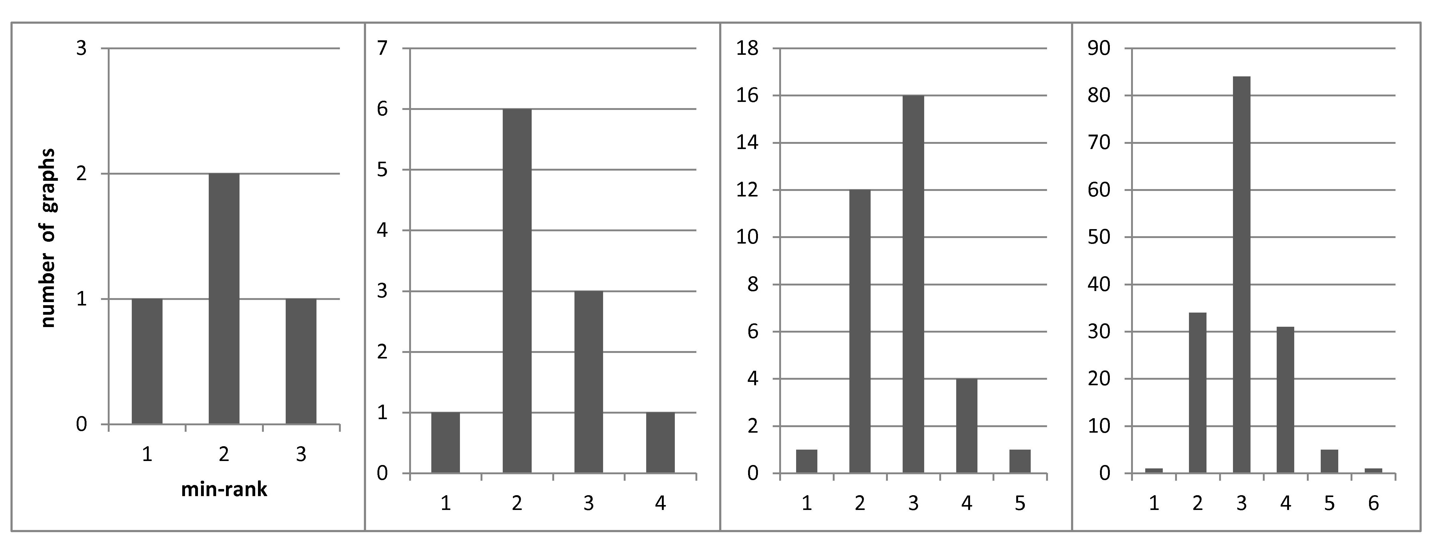
Figure 16: Min-rank distributions for graphs of orders $3$–$6$

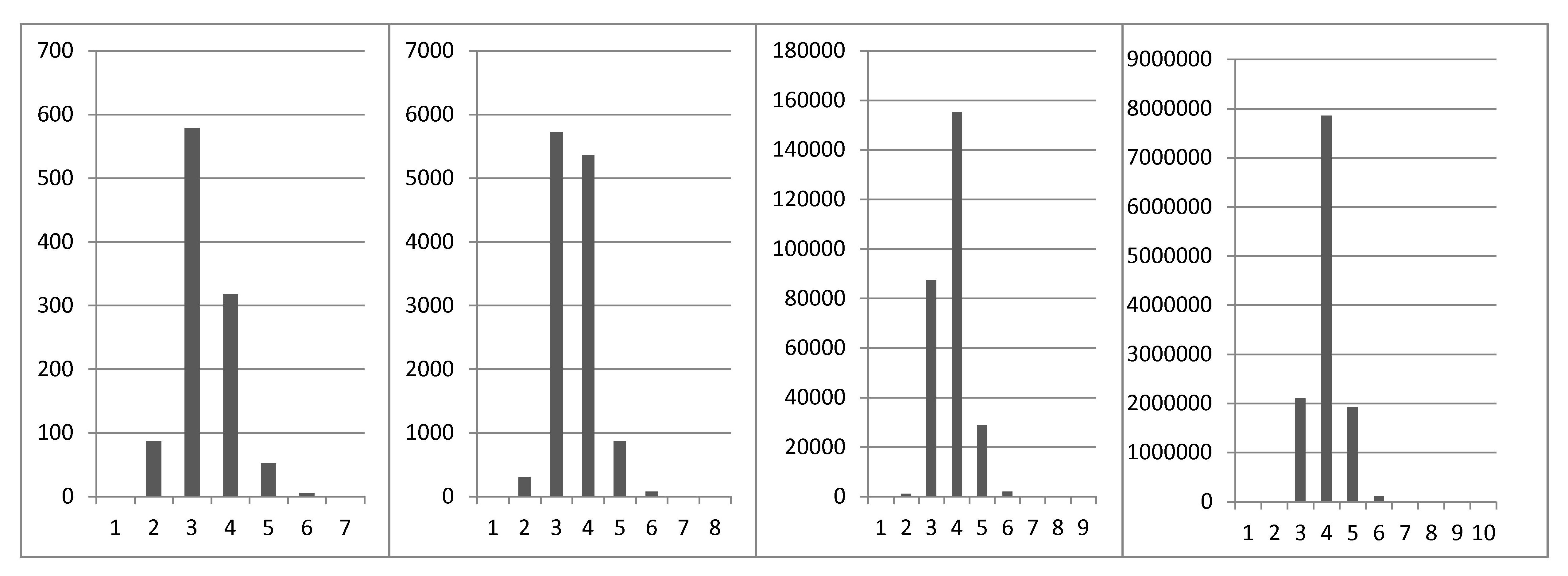
Figure 17: Min-rank distributions for graphs of orders $7$–$10$

To achieve our goal, we wrote a sub-program which used a Branch-and-Bound algorithm to find min-ranks in an exhaustive manner. When the input graph was of large size, that is, its size surpasses a given threshold, a sub-program using a SAT-solver was invoked; Otherwise, the Branch-and-Bound sub-program was used. We noticed that there are graphs of order $10$ that have around $21$–$22$ edges, for which the Branch-and-Bound sub-program could find the min-ranks in less than one second, while the SAT-based sub-program could not finish computations after $3$-$4$ hours. For graphs of order $10$, we observed that the threshold $24$, which we actually used, did work well. The most time-consuming task is to compute the min-ranks of all $12,005,618$ non-isomorphic graphs of order $10$. This task took more than four days to finish.

The charts in Figure 16 and Figure 17 present the distributions of min-ranks of non-isomorphic graphs of orders from three to ten. In each chart, the x-axis shows the minranks, and the y-axis shows the number of non-isomorphic graphs that have a certain minrank. The minranks and the corresponding matrices that achieve the minranks of all non-isomorphic graphs of orders up to $10$ are available at [12]. Interested reader may also visit [13] to calculate the min-rank of a graph.

6 Open Problems

For future research, we would like to tackle the following open problems.

Open Problem I: Currently, in order for Algorithm 1 to work, we restrict ourselves to ${\mathscr{F}}_{\mathscr{P}}(c\log(\cdot))$, the family of graphs ${\mathcal{G}}$ having a (${\mathscr{P}}$) simple tree structure $\mathscr{T}$ with $\mathsf{mdc}(\mathscr{T})\leq c\log|\mathcal{V}(\mathcal{G})|$ for some constant $c$. An intriguing question is: can we go beyond ${\mathscr{F}}_{\mathscr{P}}(c\log(\cdot))$?

Open Problem II: Find an algorithm that recognizes a member of ${\mathscr{F}}_{\mathscr{P}}(c\log(\cdot))$ in polynomial time, or show that there does not exist such an algorithm.

Open Problem III: Computation of min-ranks of graphs with $k$-multiplicity tree structures is open for every $k\geq 2$. The $2$-multiplicity tree structure is the simplest next case to consider. In such a tree structure, a node can be connected to another node by at most two edges. The idea of using a dynamic programming algorithm to compute min-ranks is almost the same. However, there are two main issues for us to tackle. Firstly, we need to study the effect on min-rank when an edge is removed from the graph. In other words, we must know the relation between $\mathsf{minrk}_{q}({\mathcal{G}})$ and $\mathsf{minrk}_{q}({\mathcal{G}}-e)$ for an edge $e$ of ${\mathcal{G}}$. This relation was investigated for outerplanar graphs by Berliner and Langberg [3, Claim 4.2, Claim 4.3]. We need to extend their result to a new scenario. Secondly, as now the two nodes in the tree structure can be connected by two edges, a recognition algorithm for graphs with $2$-multiplicity tree structures could be more complicated than that for graphs with simple tree structures.

Open Problem IV: Extending the current results to directed graphs.

7 Acknowledgments

We thank Vitaly Skachek for useful comments on the draft of the paper. We also thank Michael Langberg for providing the preprints [17], [3].

References

• [1] Ahlswede, R., Cai, N., Li, S.Y.R., Yeung, R.W.: Network information flow. IEEE Transactions on Information Theory 46, 1204–1216 (2000)
• [2] Bar-Yossef, Z., Birk, Z., Jayram, T.S., Kol, T.: Index coding with side information. In: Proceedings of the 47th Annual IEEE Symposium on Foundations of Computer Science (FOCS), pp. 197–206 (2006)
• [3] Berliner, Y., Langberg, M.: Index coding with outerplanar side information. In: Proceedings of the IEEE Symposium on Information Theory (ISIT), pp. 869–873. Saint Petersburg, Russia (2011)
• [4] Berliner, Y., Langberg, M.: Index coding with outerplanar side information (2011). Manuscript. Available at http://www.openu.ac.il/home/mikel/papers/outer.pdf
• [5] Birk, Y., Kol, T.: Informed-source coding-on-demand (ISCOD) over broadcast channels. In: Proceedings of the IEEE Conference on Computer Communications (INFOCOM), pp. 1257–1264. San Francisco, CA (1998)
• [6] Birk, Y., Kol, T.: Coding-on-demand by an informed source (ISCOD) for efficient broadcast of different supplemental data to caching clients. IEEE Transactions on Information Theory 52(6), 2825–2830 (2006)
• [7] Chartrand, G., Harary, F.: Planar permutation graphs. Annales de l’institut Henri Poincaré (B) Probabilités et Statistiques 3(4), 433–438 (1967)
• [8] Chaudhry, M.A.R., Sprintson, A.: Efficient algorithms for index coding. In: Proceedings of the IEEE Conference on Computer Communications (INFOCOM), pp. 1–4 (2008)
• [9] Chlamtac, E., Haviv, I.: Linear index coding via semidefinite programming. In: Proceedings of the 23rd Annual ACM-SIAM Symposium on Discrete Algorithms (SODA), pp. 406–419 (2012)
• [10] Chudnovsky, M., Robertson, N., Seymour, P., Thomas, R.: The strong perfect graph theorem. Annals of Mathematics 164, 51–229 (2006)
• [11] Cornuejols, G., Liu, X., Vuskovic, K.: A polynomial time algorithm for recognizing perfect graphs. Proceedings of the 48th Annual IEEE Symposium on Foundations of Computer Science (FOCS) pp. 20–27 (2003)
• [12] Dau, S.H.: (2011). web.spms.ntu.edu.sg/~daus0001/mr-small-graphs.html
• [13] Dau, S.H.: (2011). web.spms.ntu.edu.sg/~daus0001/mr.html
• [14] Eén, N., Sörensson, N.: An extensible SAT-solver. In: Theory and Applications of Satisfiability Testing, Lecture Notes in Computer Science, vol. 2919, pp. 333–336. Springer Berlin/Heidelberg (2004)
• [15] El Rouayheb, S., Sprintson, A., Georghiades, C.: On the index coding problem and its relation to network coding and matroid theory. IEEE Transactions on Information Theory 56(7), 3187–3195 (2010)
• [16] Haemers, W.: An upper bound for the Shannon capacity of a graph. Algebraic Methods in Graph Theory 25, 267–272 (1978)
• [17] Haviv, I., Langberg, M.: On linear index coding for random graphs. In: Proceedings of the IEEE International Symposium on Information Theory (ISIT), pp. 2231–2235 (2012)
• [18] Katti, S., Katabi, D., Balakrishnan, H., Médard, M.: Symbol-level network coding for wireless mesh networks. ACM SIGCOMM Computer Communication Review - Proceedings of the 2006 Conference on Applications, Technologies, Architectures, and Protocols for Computer Communications 38(4), 401–412 (2008)
• [19] Katti, S., Rahul, H., Hu, W., Katabi, D., Médard, M., Crowcroft, J.: Xors in the air: Practical wireless network coding. ACM SIGCOMM Computer Communication Review - Proceedings of the 2006 Conference on Applications, Technologies, Architectures, and Protocols for Computer Communications 36(4), 243–254 (2006)
• [20] Koetter, R., Médard, M.: An algebraic approach to network coding. IEEE/ACM Tranansactions on Networking 11, 782–795 (2003)
• [21] Langberg, M., Sprintson, A.: On the hardness of approximating the network coding capacity. In: Proceedings IEEE Symp. on Inform. Theory (ISIT), pp. 315–319. Toronto, Canada (2008)
• [22] Lovász, L.: On the Shannon capacity of a graph. IEEE Transactions on Information Theory 25, 1–7 (1979)
• [23] Lubetzky, E., Stav, U.: Non-linear index coding outperforming the linear optimum. In: Proceedings of the 48th Annual IEEE Symposium on Foundations of Computer Science (FOCS), pp. 161–168 (2007)
• [24] Peeters, R.: Orthogonal representations over finite fields and the chromatic number of graphs. Combinatorica 16(3), 417–431 (1996)
• [25] Shannon, C.E.: The zero-error capacity of a noisy channel. IRE Transactions on Information Theory 3, 3–15 (1956)
• [26] Tarjan, R.E.: A note on finding the bridges of a graph. Information Processing Letters pp. 160–161 (1974)
• [27] Wiegers, M.: Recognizing outerplanar graphs in linear time. In: Proceedings of the International Workshop WG ’86 on Graph-Theoretic Concepts in Computer Science, pp. 165–176 (1987)