Explicit secular equations for piezoacoustic surface waves:
Shear-Horizontal modes.

Abstract

Attention is given to surface waves of shear-horizontal modes in piezoelectric crystals permitting the decoupling between an elastic in-plane Rayleigh wave and a piezoacoustic anti-plane Bleustein-Gulyaev wave. Specifically, the crystals possess $\bar{4}$ symmetry (inclusive of $\bar{4}2$m, $\bar{4}3$m, and 23 classes) and the boundary is any plane containing the normal to a symmetry plane (rotated $Y$-cuts about the $Z$ axis). The secular equation is obtained explicitly as a polynomial not only for the metallized boundary condition but, in contrast to previous studies on the subject, also for other types of boundary conditions. For the metallized surface problem, the secular equation is a quadratic in the squared wave speed; for the un-metallized surface problem, it is a sextic in the squared wave speed; for the thin conducting boundary problem, it is of degree 16 in the speed. The relevant root of the secular equation can be identified and the complete solution is then found (attenuation factors, field profiles, etc.). The influences of the cut angle and of the conductance of the adjoining medium are illustrated numerically for GaAs ($\bar{4}3$m), BaLaGa₃O₇ ($\bar{4}2$m) and Bi₁₂GeO₂₀ (23). Indications are given on how to apply the method to crystals with 222 symmetry.

1 Introduction

The nature and properties of a piezoacoustic surface wave depend heavily on the crystallographic and anisotropic properties of the piezoelectric substrate, on the direction of propagation, and on the orientation of the cut (boundary) plane. For certain choices, the in-plane components of the mechanical displacement decouple from the anti-plane component, leading to two different types of surface waves namely, the Rayleigh wave, elliptically polarized in the plane containing the direction of propagation and the normal to the substrate surface, and the shear-horizontal (SH) wave, linearly polarized in the direction normal to the direction of propagation and parallel to the free surface. Moreover, either wave or both waves may be coupled to the electromagnetic fields. Of special interest are the configurations allowing for a piezoacoustic SH wave, decoupled from a purely elastic Rayleigh wave. Indeed, the former type of wave, also known as Bleustein-Gulyaev[1, 2] wave, penetrates more deeply into the substrate than the latter type; consequently, the acoustic energy is less localized and the power can be increased significantly before damage occurs (Tseng[3]) although, as pointed out by a Referee, there are exceptions to this behavior[4]. Moreover, a SH wave-based resonator is smaller than a resonator based on the propagation of a sagittally polarized surface wave (see Kadota and collaborators [5, 6]); this feature results in a downsizing of design, an attractive point for the miniaturization of mobile phones for instance, where SAW devices are used as filters. Koerber and Vogel[7, 8] identified all the cuts and rotations of axes leading to piezoacoustic SH modes; they exist for some suitable cuts and transformations in the following crystal classes: 2, 23, $\bar{4}3$m, 222, 2mm, 4, $\bar{4}$, 6, 4mm, 6mm, 32, $\bar{4}2$m, $\bar{6}$m2, 422, and 622. The main purpose of this paper is to derive explicitly the secular equation for piezoacoustic SH surface waves uncoupled from purely elastic Rayleigh waves polarized in a plane of symmetry, for a crystal in the $\bar{4}$ symmetry class (and thus for the $\bar{4}2$m, $\bar{4}3$m, and 23 classes).

Several workers addressed this topic in the wake of the seminal papers by Bleustein and by Gulyaev, but explicit results remained limited either to propagation in special directions for which one of the piezoelectric constant is zero[3, 9, 10, 11, 12, 13] or to the case where the free surface of the substrate is metallized[9], or in the weak piezoelectric coupling approximation[9, 14]. Here the crystal is cut along a plane containing the $Z$ axis and making any angle with the $XY$ crystallographic plane. Moreover the surface may be metallized, or in contact with the vacuum, or in contact with a thin conducting layer with arbitrary finite conductance. Also, no approximation is made about the strength of the piezoelectric effect. Attention is however limited to crystals with tetragonal $\bar{4}$ symmetry (inclusive of the tetragonal $\bar{4}2$m, cubic $\bar{4}3$m, and cubic 23 symmetries). This limitation is not essential but simplifies the notation to a certain extent; it is nevertheless possible to extrapolate the method presented hereafter to crystals with lower symmetries such as orthorhombic 222, as pointed out at the end of the paper. Note that the study of piezoacoustic SH surface waves in Potassium Niobate (2mm symmetry) was recently undertaken by Mozhaev and Weihnacht[15] who showed that for that class, the secular equation is a cubic in the squared wave speed.

The constitutive equations and the piezoacoustic equations for the class of crystals listed above are recalled in II.A and II.B, respectively, and some fundamental equations, which encapsulate the whole boundary value problem and its resolution, are quickly derived in II.C.

These fundamental equations are applied in Section III to the consideration of a piezoacoustic SH surface wave. A method based on the resolution of the propagation condition for partial modes first, and the resolution of the boundary value conditions next, would lead to quite an involved analysis, including the analytical examination of a quartic polynomial for the coefficients of attenuation. The method based on the fundamental equations derived in II.C circumvents the stage of the quartic and delivers directly the secular equation in polynomial form. In particular it is seen that for metallized (a.k.a. short-circuit) boundary conditions (III.A), this equation is just a quadratic in the squared wave speed, whose relevant root is readily identified. For open-circuit boundary conditions (III.B), the secular equation is also a quadratic in the squared wave speed, but it is not valid (the corresponding solution does not satisfy the boundary conditions.) For the free (non-metallized) boundary condition (III.C), the secular equation is a sextic in the squared wave speed. For the conductive thin layer boundary condition (III.D), the secular equation is a polynomial of degree 16 in the wave speed.

Once the secular equation is solved for the speed, the complete description of the wave follows naturally (IV.A), including the attenuation coefficients and the profiles for the mechanical displacement, electric potential, traction, and electrical induction. A simple check for the validity of the solution is proposed in IV.B.

The results are illustrated numerically and graphically using experimental data available for GaAs (cubic $\bar{4}3$m), BaLaGa₃O₇ (tetragonal $\bar{4}2$m) and Bi₁₂GeO₂₀ (cubic 23) in V. The range of existence of the free SH wave with respect to the angle of cut, the speeds of propagation, the amplitude of the profiles, etc. are all quantities which can be obtained numerically with as high a degree of numerical accuracy as is needed.

The paper concludes with a discussion of the merits and possible applications of the method presented, and with a chronological account of the several advances in the field, without which the results of this paper could not have been established.

2 Preliminaries

2.1 Constitutive equations

Consider a piezoelectric crystal with mass density $\rho$, possessing at most the tetragonal $\bar{4}$ symmetry (this symmetry includes the tetragonal $\bar{4}2$m, cubic $\bar{4}3$m, and cubic $23$ cases.) Let $\hat{c}_{ijkl}$, $\hat{e}_{ijk}$, and $\hat{\epsilon}_{ij}$ be its respective elastic, piezoelectric, and dielectric constants with respect to the coordinate system $XYZ$ along the crystallographic axes. Now cut the crystal by a plane containing the $Z$ axis and making an angle $\theta$ with the $XY$ plane. The new coordinate system $x_{1}x_{2}x_{3}$ (say), obtained after rotation of $XYZ$ about $Z$, is defined by

$$\begin{bmatrix}x_{1}\\ x_{2}\\ x_{3}\end{bmatrix}=\begin{bmatrix}\cos\theta&\sin\theta&0\\ -\sin\theta&\cos\theta&0\\ 0&0&1\end{bmatrix}\begin{bmatrix}X\\ Y\\ Z\end{bmatrix},$$ (1)

and so, the plane of cut is defined by $x_{2}=0$, as shown on Figure 1.

Figure 1: Rotated $Y$-cut about the $Z$ axis.

In the new coordinate system, under the electrostatic approximation for the electrical field, the stress tensor components $\sigma_{ij}$ and the electric induction components $D_{i}$ are related to the gradients of the mechanical displacement $\mathbf{u}$ and of the electrical potential $\phi$ by the constitutive relations,

$$\sigma_{ij}=c_{ijkl}u_{l,k}+e_{ijk}\phi_{,k},\quad D_{i}=e_{ikl}u_{l,k}-\epsilon_{ik}\phi_{,k},$$ (2)

where the comma denotes partial differentiation (here with respect to the $x_{k}$ coordinates). Using the Voigt contracted notation for the $c$, $e$, and $\epsilon$, these relations are written in matrix form as

$$\begin{bmatrix}\sigma_{11}\\ \sigma_{22}\\ \sigma_{33}\\ \sigma_{23}\\ \sigma_{31}\\ \sigma_{12}\\ D_{1}\\ D_{2}\\ D_{3}\end{bmatrix}=\begin{bmatrix}c_{11}&c_{12}&c_{13}&0&0&c_{16}&0&0&e_{31}\\ c_{12}&c_{11}&c_{13}&0&0&-c_{16}&0&0&-e_{31}\\ c_{13}&c_{13}&c_{33}&0&0&0&0&0&0\\ 0&0&0&c_{44}&0&0&e_{14}&-e_{15}&0\\ 0&0&0&0&c_{44}&0&e_{15}&e_{14}&0\\ c_{16}&-c_{16}&0&0&0&c_{66}&0&0&e_{36}\\ 0&0&0&e_{14}&e_{15}&0&-\epsilon_{11}&0&0\\ 0&0&0&-e_{15}&e_{14}&0&0&-\epsilon_{11}&0\\ e_{31}&-e_{31}&0&0&0&e_{36}&0&0&-\epsilon_{33}\end{bmatrix}\begin{bmatrix}u_{1,1}\\ u_{2,2}\\ u_{3,3}\\ u_{2,3}+u_{3,2}\\ u_{3,1}+u_{1,3}\\ u_{1,2}+u_{2,1}\\ \phi_{,1}\\ \phi_{,2}\\ \phi_{,3}\\ \end{bmatrix}.$$ (3)

Explicitly, the $c_{ij}$ and $e_{ij}$ are deduced from the $\hat{c}_{ij}$ and $\hat{e}_{ij}$ in $XYZ$ by well-known relationships. In particular,

$$c_{44}=\hat{c}_{44},\quad\epsilon_{11}=\hat{\epsilon}_{11},$$

$$e_{14}=\hat{e}_{14}\cos 2\theta-\hat{e}_{15}\sin 2\theta,$$

$$e_{15}=\hat{e}_{15}\cos 2\theta+\hat{e}_{14}\sin 2\theta.$$ (4)

2.2 Piezoacoustic equations

Now consider the propagation of an anti-plane (SH) inhomogeneous wave in the half-space $x_{2}\geq 0$, travelling with speed $v$ and wave number $k$ in the $x_{1}$ direction, with attenuation in the $x_{2}$ direction. It is known[16] that for the crystals under consideration this wave decouples entirely from its in-plane counterpart, a purely elastic two-component Rayleigh wave. Thus the wave is modelled as $u_{1}=u_{2}=0$, and

$$\{u_{3},\phi\}=\{U_{3}(kx_{2}),\varphi(kx_{2})\}e^{ik(x_{1}-vt)},$$ (5)

for some yet unknown functions $U_{3}$ and $\varphi$ of $kx_{2}$. Accordingly, the constitutive equations Eq. (2) lead to similar forms for the stress and electrical components,

$$\{\sigma_{ij},D_{i}\}=ik\{t_{ij}(kx_{2}),d_{i}(kx_{2})\}e^{ik(x_{1}-vt)},$$ (6)

where $t_{11}=t_{22}=t_{12}=d_{3}=0$, and

$$t_{33}=c_{13}U_{1}-ic_{11}U^{\prime}_{2},$$

$$t_{32}=-ic_{44}U^{\prime}_{3}+e_{14}\varphi+ie_{15}\varphi^{\prime},$$

$$t_{31}=c_{44}U_{3}+e_{15}\varphi-ie_{14}\varphi^{\prime},$$

$$d_{1}=e_{15}U_{3}-ie_{14}U^{\prime}_{3}-\epsilon_{11}\varphi,$$

$$d_{2}=e_{14}U_{3}+ie_{15}U^{\prime}_{3}+i\epsilon_{11}\varphi^{\prime}.$$ (7)

Here and hereafter, the prime denotes differentiation with respect to the variable $kx_{2}$.

Using the above-introduced functions $U_{3}$, $\varphi$, $t_{ij}$, $d_{i}$, the classical equations of piezoacoustics,

$$\sigma_{ij,j}=\rho u_{i,tt},\quad D_{i,i}=0,$$ (8)

reduce to

$$-t_{13}+it^{\prime}_{32}=-XU_{3},\quad-d_{1}+id^{\prime}_{2}=0,$$ (9)

where $X:=\rho v^{2}$.

When the region $x_{2}<0$ above the crystal is the vacuum (permeability: $\epsilon_{0}$) and the surface $x_{2}=0$ remains free of tractions, then the boundary value problem corresponding to Eq. (9) is that of piezoacoustic (Bleustein-Gulyaev) SH surface waves.

2.3 Fundamental equations for the resolution

The method of resolution rests on the property that the piezoacoustic equations (9) can be written in the form,

$$\mbox{\boldmath$\xi$}^{\prime}=i\mathbf{N}\mbox{\boldmath$\xi$},\quad\text{where}\quad\mbox{\boldmath$\xi$}(kx_{2})=[U_{3},\varphi,t_{32},d_{2}]^{\text{T}},$$ (10)

and $\mathbf{N}$ is a real 4$\times$4 matrix which, brought up to any positive or negative integer power $n$ has the following block structure,

$$\mathbf{N}^{n}=\begin{bmatrix}\mathbf{N^{(n)}_{1}}&\mathbf{N^{(n)}_{2}}\\ \mathbf{K^{(n)}}&(\mathbf{N^{(n)}_{1}})^{\mathrm{T}}\end{bmatrix},\quad\text{with}\quad\mathbf{K^{(n)}}=(\mathbf{K^{(n)}})^{\mathrm{T}},\quad\mathbf{N^{(n)}_{2}}=(\mathbf{N^{(n)}_{2}})^{\mathrm{T}},$$ (11)

where ${}^{\text{T}}$ denotes the transpose, and where the submatrices of $\mathbf{N}^{n}$ are $2\times 2$ matrices. The first-order differential form Eq. (10) of the piezoacoustic equations dates back to Kraut[17], and before that, to Stroh[18] and others (see Fahmy and Adler[19] for references) for the purely elastic case. The subsequent analysis below builds upon several crucial contributions, which are listed and put into context at the very end of this article.

Now, because the wave amplitude must vanish away from $x_{2}=0$, $\mbox{\boldmath$\xi$}(kx_{2})$ is such that

$$\mbox{\boldmath$\xi$}(\infty)=\mathbf{0}.$$ (12)

Clearly, pre-multiplication of $\mathbf{N}^{n}$ by $\widehat{\mathbf{I}}$ defined as,

$$\widehat{\mathbf{I}}=\begin{bmatrix}0&\mathbf{1}\\ \mathbf{1}&0\end{bmatrix},\quad\text{where}\quad\mathbf{1}=\begin{bmatrix}1&0\\ 0&1\end{bmatrix},$$ (13)

produces a symmetric matrix,

$$\widehat{\mathbf{I}}\mathbf{N}^{n}=\begin{bmatrix}\mathbf{K^{(n)}}&(\mathbf{N^{(n)}_{1}})^{\mathrm{T}}\\ \mathbf{N^{(n)}_{1}}&\mathbf{N^{(n)}_{2}}\end{bmatrix}=(\widehat{\mathbf{I}}\mathbf{N}^{n})^{\text{T}},$$ (14)

so that taking the scalar product on both sides of Eq. (10) by $\widehat{\mathbf{I}}\mathbf{N}^{n}\overline{\mbox{\boldmath$\xi$}}$, where the overbar denotes the complex conjugate, leads to $\overline{\mbox{\boldmath$\xi$}}\cdot\widehat{\mathbf{I}}\mathbf{N}^{n}\mbox{\boldmath$\xi$}^{\prime}=i\overline{\mbox{\boldmath$\xi$}}\cdot\widehat{\mathbf{I}}\mathbf{N}^{n+1}\mbox{\boldmath$\xi$}$, the right hand-side of which is purely imaginary. Taking the real part and integrating yields $\overline{\mbox{\boldmath$\xi$}}\cdot\widehat{\mathbf{I}}\mathbf{N}^{n}\mbox{\boldmath$\xi$}=$ const. $=0$ (by Eq. (12)), and in particular,

$$\overline{\mbox{\boldmath$\xi$}}(0)\cdot\widehat{\mathbf{I}}\mathbf{N}^{n}\mbox{\boldmath$\xi$}(0)=0.$$ (15)

These fundamental equations[20, 21, 22] allow for a completely analytical derivation of the secular equation, for a great variety of boundary conditions. Note that because $\mathbf{N}$ is a $4\times 4$ matrix, there are at most three independent fundamental equations according to the Cayley-Hamilton theorem. Any choice of three different integers $n$ is legitimate, although the choice $n=-1,1,2$ seems to yield the most compact expressions for the components of $\mathbf{N}^{n}$.

3 Secular equations

For the piezoacoustic (Bleustein-Gulyaev) shear-horizontal wave, the matrix $\mathbf{N}$ in Eq. (10) is written in compact form using the following quantity,

$$\kappa^{2}=\dfrac{e^{2}_{14}}{\epsilon_{11}c_{44}+e_{15}^{2}},$$ (16)

as

$$\mathbf{N}=\begin{bmatrix}\vspace{6pt}\dfrac{e_{15}}{e_{14}}\kappa^{2}&-\dfrac{\epsilon_{11}}{e_{14}}\kappa^{2}&\dfrac{\epsilon_{11}}{e_{14}^{2}}\kappa^{2}&-\dfrac{e_{15}}{e_{14}^{2}}\kappa^{2}\\ \vspace{6pt}\dfrac{c_{44}}{e_{14}}\kappa^{2}&\dfrac{e_{15}}{e_{14}}\kappa^{2}&-\dfrac{e_{15}}{e_{14}^{2}}\kappa^{2}&-\dfrac{c_{44}}{e_{14}^{2}}\kappa^{2}\\ \vspace{6pt}X-c_{44}(1+\kappa^{2})&-e_{15}(1+\kappa^{2})&\dfrac{e_{15}}{e_{14}}\kappa^{2}&\dfrac{c_{44}}{e_{14}}\kappa^{2}\\ \vspace{6pt}-e_{15}(1+\kappa^{2})&\epsilon_{11}(1+\kappa^{2})&-\dfrac{\epsilon_{11}}{e_{14}}\kappa^{2}&\dfrac{e_{15}}{e_{14}}\kappa^{2}\end{bmatrix}.$$ (17)

Note that $\mathbf{N}$ is indeed of the form Eq. (11). To express explicitly integer powers of $\mathbf{N}$, it proves convenient to use scalar multiples of the matrix $\widehat{\mathbf{I}}\mathbf{N}^{n}$, for which the fundamental equations Eq. (15) are also valid. For instance, the fundamental equations (15) also hold at $n=2,-1$ when $\widehat{\mathbf{I}}\mathbf{N}^{n}$ is replaced with $\mathbf{M^{(2)}}$, $\mathbf{M^{(-1)}}$ respectively, defined by

$$\mathbf{M^{(2)}}=\dfrac{e_{14}}{e_{15}\kappa^{2}}\widehat{\mathbf{I}}\mathbf{N}^{2},\quad\mathbf{M^{(-1)}}=(\dfrac{\epsilon_{11}c_{44}}{e_{14}^{2}}\kappa^{2}X-1)\widehat{\mathbf{I}}\mathbf{N}^{-1}.$$ (18)

These symmetric matrices are given explicitly by their components,

$$M^{(2)}_{11}=2[X-2c_{44}(1+\kappa^{2})], M^{(2)}_{12}=-\dfrac{\epsilon_{11}}{e_{15}}X+2\dfrac{\epsilon_{11}c_{44}-e_{15}^{2}}{e_{15}}(1+\kappa^{2}),$$

$$M^{(2)}_{22}=4\epsilon_{11}(1+\kappa^{2}), M^{(2)}_{13}=\dfrac{\epsilon_{11}}{e_{14}e_{15}}X-\dfrac{\epsilon_{11}c_{44}-e_{15}^{2}}{e_{14}e_{15}}(1+2\kappa^{2}),$$

$$M^{(2)}_{23}=-2\dfrac{\epsilon_{11}}{e_{14}}(1+2\kappa^{2}), M^{(2)}_{33}=4\dfrac{\epsilon_{11}}{e_{14}^{2}}\kappa^{2},$$

$$M^{(2)}_{14}=-\dfrac{1}{e_{14}}X+2\dfrac{c_{44}}{e_{14}}(1+2\kappa^{2}), M^{(2)}_{24}=-\dfrac{\epsilon_{11}c_{44}-e_{15}^{2}}{e_{14}e_{15}}(1+2\kappa^{2}),$$

$$M^{(2)}_{34}=2\dfrac{\epsilon_{11}c_{44}-e_{15}^{2}}{e_{14}^{2}e_{15}}\kappa^{2}, M^{(2)}_{44}=-4\dfrac{c_{44}}{e_{14}^{2}}\kappa^{2},$$ (19)

and

$$M^{(-1)}_{11}=(1+\dfrac{\epsilon_{11}c_{44}}{e_{14}^{2}})\kappa^{2}X-c_{44}(1+\kappa^{2}), M^{(-1)}_{12}=-\dfrac{\epsilon_{11}e_{15}}{e_{14}^{2}}\kappa^{2}X+e_{15}(1+\kappa^{2}),$$

$$M^{(-1)}_{22}=-\dfrac{\epsilon_{11}^{2}}{e_{14}^{2}}\kappa^{2}X+\epsilon_{11}(1+\kappa^{2}), M^{(-1)}_{13}=\dfrac{e_{15}}{e_{14}}\kappa^{2},$$

$$M^{(-1)}_{23}=\dfrac{\epsilon_{11}}{e_{14}}\kappa^{2}, M^{(-1)}_{33}=\dfrac{\epsilon_{11}}{e_{14}^{2}}\kappa^{2},$$

$$M^{(-1)}_{14}=\dfrac{X-c_{44}}{e_{14}}\kappa^{2}, M^{(-1)}_{24}=\dfrac{e_{15}}{e_{14}}\kappa^{2},$$

$$M^{(-1)}_{34}=\dfrac{e_{15}}{e_{14}^{2}}\kappa^{2}, M^{(-1)}_{44}=\dfrac{X-c_{44}}{e_{14}^{2}}\kappa^{2}.$$ (20)

Now all the required equations and quantities are in place to treat various electrical boundary value problems.

3.1 Metallized (short-circuit) boundary condition

Here the surface of the crystal is coated with a thin metallic film, with thickness negligible when compared to the wavelength, and brought to a zero electrical potential. Moreover, the coating still allows the surface to remain free of mechanical tractions. Then

$$\sigma_{23}=0,\>\phi=0,\text{ at }x_{2}=0,\quad\text{so that}\quad\mbox{\boldmath$\xi$}(0)=[U_{3}(0),0,0,d_{2}(0)]^{\text{T}}.$$ (21)

Writing $\mbox{\boldmath$\xi$}(0)=U_{3}(0)[1,0,0,\alpha]$, where $\alpha=d_{2}(0)/U_{3}(0)$ is complex, the fundamental equations (15) for $\widehat{\mathbf{I}}\mathbf{N}$ ($n=1$), $\mathbf{M^{(2)}}$ ($n=2$), and $\mathbf{M^{(-1)}}$ ($n=-1$) lead to the following homogeneous system of equations,

$$\begin{bmatrix}N_{31}&N_{21}&N_{24}\\ M^{(2)}_{11}&M^{(2)}_{14}&M^{(2)}_{44}\\ M^{(-1)}_{11}&M^{(-1)}_{14}&M^{(-1)}_{44}\end{bmatrix}\begin{bmatrix}1\\ \alpha+\overline{\alpha}\\ \alpha\overline{\alpha}\end{bmatrix}=\begin{bmatrix}0\\ 0\\ 0\end{bmatrix}.$$ (22)

For a non-trivial solution to exist, the determinant of the system’s matrix must be zero. Factoring out common factors, this condition reads

$$\begin{vmatrix}X-c_{44}(1+\kappa^{2})&c_{44}\kappa^{2}&-c_{44}\\ 2[X-2c_{44}(1+\kappa^{2})]&-X+2c_{44}(1+2\kappa^{2})&-4c_{44}\\ (1+\dfrac{\epsilon_{11}c_{44}}{e_{14}^{2}})\kappa^{2}X-c_{44}(1+\kappa^{2})&(X-c_{44})\kappa^{2}&X-c_{44}\end{vmatrix}=0.$$ (23)

When $X=0$, the first column in the determinant becomes proportional to the third, and the determinant is zero. Hence $X$ is a factor of the determinant; the remaining factor is a quadratic in $X$,

$$X^{2}-c_{44}(\dfrac{3\epsilon_{11}c_{44}+4e_{14}^{2}+4e_{15}^{2}}{\epsilon_{11}c_{44}+e_{15}^{2}})X+2c_{44}^{2}(\dfrac{\epsilon_{11}c_{44}+2e_{14}^{2}+2e_{15}^{2}}{\epsilon_{11}c_{44}+e_{15}^{2}})=0,$$ (24)

that is, the explicit secular equation for piezoacoustic (Bleustein-Gulyaev) anti-plane surface waves on a metallized tetragonal $\bar{4}$ (or tetragonal $\bar{4}2$m, or cubic $\bar{4}3$m, $23$) crystal, cut along any plane containing the $Z$ axis.

This equation being a quadratic in $X$, it is solved explicitly and it yields a priori two roots. The selection is made by considering the known speed of a Bleustein-Gulyaev surface wave in a cubic $\bar{4}3$m or $23$ crystal when $\theta=45^{\text{o}}$. Then the root of the quadratic corresponding to the plus sign is $X=\rho v^{2}=2c_{44}$, and the root corresponding to the minus sign is

$$\rho v^{2}=c_{44}(1+\dfrac{e_{15}^{2}}{c_{44}\epsilon_{11}+e_{15}^{2}})=c_{44}(1+\dfrac{\hat{e}_{14}^{2}}{c_{44}\epsilon_{11}+\hat{e}_{14}^{2}}),$$ (25)

in accordance with Tseng[3] (see also Koerber and Vogel[7], Alburque and Chao[10], Velasco[11], Bright and Hunt[13]). By continuity with the other cases ($\bar{4}$, $\bar{4}2$m, $\bar{4}3$m, $23$, $\theta\neq 45^{\text{o}}$), the speed of the generic Bleustein-Gulyaev wave found from the secular equation (24) is $v_{\text{BGm}}$, given by

$$\dfrac{\rho v_{\text{BGm}}^{2}}{c_{44}}=\dfrac{3\epsilon_{11}c_{44}+4e_{14}^{2}+4e_{15}^{2}-[(\epsilon_{11}c_{44}+4e_{14}^{2})^{2}+(4e_{14}e_{15})^{2}]^{\textstyle{\frac{1}{2}}}}{2(\epsilon_{11}c_{44}+e_{15}^{2})}.$$ (26)

For tetragonal $\bar{4}2$m, cubic $\bar{4}3$m, or cubic $23$ crystals, $\hat{e}_{15}=0$ and by Eq. (2.1), this expression reduces to

$$\dfrac{\rho v_{\text{BGm}}^{2}}{c_{44}}=\dfrac{3+4\hat{\chi}^{2}-[(1+4\hat{\chi}^{2}\cos^{2}2\theta)^{2}+4\hat{\chi}^{4}\sin^{2}4\theta]^{\textstyle{\frac{1}{2}}}}{2(1+\hat{\chi}^{2}\sin^{2}2\theta)},$$ (27)

as proved by Braginskiĭ and Gilinskiĭ[9] using a different method. In Eq. (27), $\hat{\chi}^{2}=\hat{e}_{14}^{2}/(\epsilon_{11}c_{44})$ is the “piezoelectric coupling coefficient” for bulk waves.

3.2 Electrically open boundary condition

The substrate is said to be “mechanically free, electrically open” (Ingebrigsten[23], Lothe and Barnett[24]) when

$$\sigma_{32}=0,\;D_{2}=0,\text{ at }x_{2}=0,\quad\text{so that}\quad\mbox{\boldmath$\xi$}(0)=[U_{3}(0),\varphi(0),0,0]^{\text{T}}.$$ (28)

Writing $\mbox{\boldmath$\xi$}(0)=U_{3}(0)[1,\alpha,0,0]$, where $\alpha=\varphi(0)/U_{3}(0)$ is complex, the fundamental equations (15) for $\widehat{\mathbf{I}}\mathbf{N}$ ($n=1$), $\mathbf{M^{(2)}}$ ($n=2$), and $\mathbf{M^{(-1)}}$ ($n=-1$) lead to the following homogeneous system of equations,

$$\begin{bmatrix}N_{31}&N_{32}&N_{42}\\ M^{(2)}_{11}&M^{(2)}_{12}&M^{(2)}_{22}\\ M^{(-1)}_{11}&M^{(-1)}_{12}&M^{(-1)}_{22}\end{bmatrix}\begin{bmatrix}1\\ \alpha+\overline{\alpha}\\ \alpha\overline{\alpha}\end{bmatrix}=\begin{bmatrix}0\\ 0\\ 0\end{bmatrix}.$$ (29)

For a non-trivial solution to exist, the determinant of the system’s matrix must be zero. Its components are given in Eq. (17), Eq. (3), and Eq. (3). As in the short-circuit configuration, at $X=0$ the first and third columns in the determinant become both proportional to $[1,4,1]^{\text{T}}$ and so $X$ is a factor of the determinant; the remaining factor is a quadratic in $X$,

$$\dfrac{\epsilon_{11}^{2}}{e_{14}^{2}}\kappa^{2}X^{2}-\epsilon_{11}(1+\kappa^{2})[3-(1+4\dfrac{e_{15}^{2}}{e_{14}^{2}})\kappa^{2}]X+2(1+\kappa^{2})^{2}(\epsilon_{11}c_{44}-e_{14}^{2}-e_{15}^{2})=0.$$ (30)

At this stage, an important point must be raised. Although this secular equation might seem legitimate at first sight, it must be recalled that it was obtained through a process based on the fundamental equations (15) which, due to the involvement of integer powers of the matrix $\mathbf{N}$, might generate spurious secular equations. In fact, it has been proved[24, 9] that the Bleustein-Gulyaev wave does not exist for open circuit boundary conditions. Hence the secular equation Eq. (30) is not valid. It is given here for completeness and to illustrate one limitation of the fundamental equations approach. However, as is seen in IV.B, a simple check can be done to realize whether the speed given by an explicit secular equation is valid or not.

3.3 Free boundary condition

In the general case of a non-metallized, mechanically free boundary, the tangential component of the electric field and the normal component of the electric induction are continuous across the substrate/vacuum interface. These continuities lead to the relationship (e.g. Dieulesaint and Royer [25] p.288),

$$d_{2}(0)=i\epsilon_{0}\varphi(0),\quad\text{so that}\quad\mbox{\boldmath$\xi$}(0)=\varphi(0)[\alpha,1,0,i\epsilon_{o}]^{\text{T}},$$ (31)

where $\alpha=\alpha_{1}+i\alpha_{2}=U_{3}(0)/\varphi(0)$ is complex. Now the fundamental equations (15) for $\widehat{\mathbf{I}}\mathbf{N}$ ($n=1$), $\mathbf{M^{(2)}}$ ($n=2$), and $\mathbf{M^{(-1)}}$ ($n=-1$) lead to a non-homogeneous linear system of equations,

$$\begin{bmatrix}N_{32}&\epsilon_{0}N_{21}&N_{31}\\ M^{(2)}_{12}&\epsilon_{0}M^{(2)}_{14}&M^{(2)}_{11}\\ M^{(-1)}_{12}&\epsilon_{0}M^{(-1)}_{14}&M^{(-1)}_{11}\end{bmatrix}\begin{bmatrix}2\alpha_{1}\\ 2\alpha_{2}\\ \alpha_{1}^{2}+\alpha_{2}^{2}\end{bmatrix}=\begin{bmatrix}-N_{42}-\epsilon_{0}^{2}N_{24}\\ -M^{(2)}_{22}-\epsilon_{0}^{2}M^{(2)}_{44}\\ -M^{(-1)}_{22}-\epsilon_{0}^{2}M^{(-1)}_{44}\end{bmatrix}.$$ (32)

By Cramer’s rule, the unique solution to this system is

$$2\alpha_{1}=\Delta_{1}/\Delta,\quad 2\alpha_{2}=\Delta_{2}/\Delta,\quad\alpha_{1}^{2}+\alpha_{2}^{2}=\Delta_{3}/\Delta,$$ (33)

where $\Delta$ is the determinant of the $3\times 3$ matrix in Eq. (32), with components given in Eq. (17), Eq. (3), and Eq. (3), and the $\Delta_{k}$ are the determinants obtained by replacing this matrix’s $k$-th column with the vector on the right hand-side of Eq. (32). It follows from Eq. (33) that

$$\Delta_{1}^{2}+\Delta_{2}^{2}-4\Delta\Delta_{3}=0,$$ (34)

which is the explicit secular equation for piezoacoustic (Bleustein-Gulyaev) anti-plane surface waves on a non-metallized, mechanically free $\bar{4}$ (or $\bar{4}2$m, $\bar{4}3$m, $23$) crystal, cut along any plane containing the $Z$ axis.

The expansions of the determinants $\Delta$, …, $\Delta_{3}$ are lengthy and are not displayed here, but they are easily computed by using the components Eq. (17), Eq. (3), and Eq. (3). It turns out that $\Delta$ factorizes into the product of $\epsilon_{0}$ and a cubic in $X$ which is independent of $\epsilon_{0}$, while $\Delta_{1}$ (resp. $\Delta_{2}$, $\Delta_{3}$) factorizes into the product of $\epsilon_{0}X$ (resp. $X$, $\epsilon_{0}$) and a polynomial which is quadratic in $X$ and linear in $\epsilon_{0}^{2}$. The resulting secular equation (34) is a sextic in $X$ and a cubic in $\epsilon_{0}^{2}$, with the coefficient of the $\epsilon_{0}^{6}$ term proportional to the “metallized secular equation” (24) and the coefficient of the $\epsilon_{0}^{0}$ term proportional to the (non-valid) “open circuit secular equation” (30).

It is emphasized again that, as in III.B, great care must be taken to ensure that the speed given by the secular equation Eq. (34) leads to a valid solution. This point is discussed in IV.B.

3.4 Thin conducting layer boundary condition

As a final type of boundary condition, consider that the semi-infinite substrate is covered with a metallic film with thickness $h$ and conductance $\gamma$, where $h$ is assumed to be so small with respect to the acoustic wavelength that the effects of mechanical loading can be neglected. Then the permeability of the region $x_{2}<0$ close to the interface is changed from $\epsilon_{0}$ (see previous Subsection) to $\epsilon_{0}-i\epsilon$ (see Royer and Dieulesaint[26], p. 301), with $\epsilon=\gamma h/v$. Replacing the former quantity with the latter in the previous Subsection leads to similar results as above, except that the $3\times 3$ matrix and the right hand-side of Eq. (32) are now replaced with

$$\begin{bmatrix}N_{32}+\epsilon N_{21}&\epsilon_{0}N_{21}&N_{31}\\ M^{(2)}_{12}+\epsilon M^{(2)}_{14}&\epsilon_{0}M^{(2)}_{14}&M^{(2)}_{11}\\ M^{(-1)}_{12}+\epsilon M^{(-1)}_{14}&\epsilon_{0}M^{(-1)}_{14}&M^{(-1)}_{11}\end{bmatrix},\\ \text{and}\quad\begin{bmatrix}-N_{42}-2\epsilon N_{22}-(\epsilon_{0}^{2}+\epsilon^{2})N_{24}\\ -M^{(2)}_{22}-2\epsilon M^{(2)}_{24}-(\epsilon_{0}^{2}+\epsilon^{2})M^{(2)}_{44}\\ -M^{(-1)}_{22}-2\epsilon M^{(-1)}_{24}-(\epsilon_{0}^{2}+\epsilon^{2})M^{(-1)}_{44}\end{bmatrix},$$ (35)

respectively. Then the secular equation is Eq. (34) where $\Delta$, …, $\Delta_{3}$ are appropriately changed. Because here the quantity $\epsilon$ depends upon $v$, the secular equation is a polynomial in the speed of degree higher than in the previous Subsection, namely it is a polynomial of degree 16 in $v$.

4 Construction of the solutions

4.1 Description of the wave

Once a wave speed is determined from the secular equation, it is a rather straightforward matter to construct the corresponding complete solution. Indeed, the anti-plane mechanical displacement $u_{3}$, the electrical potential $\phi$, the shear stress $\sigma_{32}$, and the electric induction $D_{2}$ are given by

$$[u_{3},\phi,\sigma_{32},D_{2}](x_{1},x_{2},t)=\Re\{[U_{3},\varphi,ikt_{32},ikd_{2}](kx_{2})e^{ik(x_{1}-vt)}\}.$$ (36)

Here $U_{3}$, $\varphi$, $t_{32}$, $d_{2}$ are the components of $\xi$, solution to $\mbox{\boldmath$\xi$}^{\prime}=i\mathbf{N}\mbox{\boldmath$\xi$}$. Taking $\xi$ in exponential form leads to the following decaying solution,

$$\mbox{\boldmath$\xi$}=\beta_{1}\mbox{\boldmath$\xi^{1}$}e^{ikq_{1}x_{2}}+\beta_{2}\mbox{\boldmath$\xi^{2}$}e^{ikq_{2}x_{2}},$$ (37)

where $\beta_{1}$, $\beta_{2}$ are constants, $q_{1}$, $q_{2}$ are the two roots with positive imaginary part to the inhomogeneous wave propagation condition: $\text{det }(\mathbf{N}-q\mathbf{1})=0$, and the $\xi^{i}$ satisfy: $\mathbf{N}\mbox{\boldmath$\xi^{i}$}=q_{i}\mbox{\boldmath$\xi^{i}$}$.

Explicitly, the $q_{i}$ are roots of the quartic,

$$(\epsilon_{11}c_{44}+e_{15}^{2})q^{4}-4e_{14}e_{15}q^{3}-[\epsilon_{11}(X-2c_{44})-4e_{14}^{2}+2e_{15}^{2}]q^{2}\\ +4e_{14}e_{15}q+e_{15}^{2}-\epsilon_{11}(X-c_{44})=0,$$ (38)

and the $\xi^{i}$ are proportional to any column vector of the matrix adjoint to $\mathbf{N}-q_{i}\mathbf{1}$, the third one say. Hence,

$$\mbox{\boldmath$\xi^{i}$}=\left[\dfrac{e_{14}}{c_{44}}a_{i},\>b_{i},\>e_{14}^{2}f_{i},\>\dfrac{e_{14}^{2}}{c_{44}}g_{i}\right]^{\text{T}},$$ (39)

where the non-dimensional real quantities $a_{i}$, $b_{i}$, $f_{i}$, $g_{i}$ ($i=1,2$) are given by

$$a_{i}=-\dfrac{\epsilon_{11}c_{44}}{e_{14}^{2}}(q_{i}^{2}+1),\quad b_{i}=\dfrac{e_{15}}{e_{14}}(q_{i}^{2}-1)-2q_{i},$$

$$f_{i}=\dfrac{e_{15}}{e_{14}}(3q_{i}^{2}-1)-\dfrac{e_{15}^{2}}{e_{14}^{2}}q_{i}(q_{i}^{2}-1)-\dfrac{\epsilon_{11}c_{44}}{e_{14}^{2}}q_{i}(q_{i}^{2}+1)-2q_{i},$$

$$g_{i}=\dfrac{\epsilon_{11}c_{44}}{e_{14}^{2}}(q_{i}^{2}+2\dfrac{e_{15}}{e_{14}}q_{i}-1).$$ (40)

Finally, the ratio $\beta_{2}/\beta_{1}$ comes from the condition that the third component of $\mbox{\boldmath$\xi$}(0)$, proportional to $t_{23}(0)$, must be zero, so that $\beta_{2}/\beta_{1}=-f_{1}/f_{2}$.

4.2 Validity of the solution

Once a wave solution has been constructed, its validity must be checked that is, it must satisfy the boundary conditions.

Thus, for a solution to the short-circuit problem (III.A), it must be checked that $\varphi(0)=\beta_{1}b_{1}+\beta_{2}b_{2}$ and $t_{32}(0)=\beta_{1}e_{14}f_{1}+\beta_{2}e_{14}f_{2}$ are indeed equal to zero. These conditions are equivalent to checking that

$$\begin{vmatrix}b_{1}&b_{2}\\ f_{1}&f_{2}\end{vmatrix}=0.$$ (41)

For a solution to the open-circuit problem (III.B), it must be checked that $t_{32}(0)=\beta_{1}e_{14}f_{1}+\beta_{2}e_{14}f_{2}$ and $d_{2}(0)=\beta_{1}(e_{14}^{2}/c_{44})g_{1}+\beta_{2}(e_{14}^{2}/c_{44})g_{2}$ are equal to zero. These conditions are equivalent to checking that $\begin{vmatrix}f_{1}&f_{2}\\ g_{1}&g_{2}\end{vmatrix}=0$. As expected[24, 9], this condition is never satisfied.

For a solution to the free boundary problem (III.C), it must be checked that $t_{32}(0)=\beta_{1}e_{14}f_{1}+\beta_{2}e_{14}f_{2}=0$ and that $d_{2}(0)=i\epsilon_{0}\varphi(0)$ that is, $\beta_{1}(e_{14}^{2}/c_{44})g_{1}+\beta_{2}(e_{14}^{2}/c_{44})g_{2}=i\epsilon_{0}(\beta_{1}b_{1}+\beta_{2}b_{2})$. These conditions are equivalent to checking that

$$\begin{vmatrix}f_{1}&f_{2}\\ \dfrac{e_{14}^{2}}{c_{44}\epsilon_{0}}g_{1}-ib_{1}&\dfrac{e_{14}^{2}}{c_{44}\epsilon_{0}}g_{2}-ib_{2}\end{vmatrix}=0.$$ (42)

In general, this condition is met only for a limited range of the cut angle $\theta$.

Finally, for a solution to the thin conducting layer boundary problem (III.D), it must be checked that $t_{32}(0)=0$ and that $d_{2}(0)=(\epsilon+i\epsilon_{0})\varphi(0)$. These conditions are equivalent to checking that

$$\begin{vmatrix}f_{1}&f_{2}\\ \dfrac{e_{14}^{2}}{c_{44}(\epsilon_{0}-i\epsilon)}g_{1}-ib_{1}&\dfrac{e_{14}^{2}}{c_{44}(\epsilon_{0}-i\epsilon)}g_{2}-ib_{2}\end{vmatrix}=0.$$ (43)

5 Examples

In this Section, the secular equations derived in III and the tests presented in IV are employed to find numerically the wave speed and its range of existence for three crystals, one with cubic $\bar{4}3$m symmetry, one with tetragonal $\bar{4}2$m symmetry, and one with cubic 23 symmetry. Data collected from the specialized literature are used for the values of the mass densities, of the stiffnesses, and of the piezoelectric and dielectric constants. In order to graph the depth profiles, a frequency of 100 MHz and a mechanical displacement of $10^{-13}$ m at $x_{2}=0$ are picked, to fix the ideas. Note that at a 45^∘ angle of cut, the profiles present pure (non-oscillating) exponential decay, because the propagation condition (38) is a biquadratic and the corresponding roots are purely imaginary; they are essentially similar to those displayed by Bright and Hunt[13]. Here the profiles are computed at angles $\neq 45^{\circ}$.

5.1 AlAs

For Aluminum Arsenide ($\bar{4}3$m symmetry) the physical quantities of interest are[27]: $\rho=3760$ kg$\cdot$m^-3, $c_{44}=58.9\times 10^{9}$ N$\cdot$m^-2, $\hat{e}_{14}=-0.225$ C$\cdot$m^-2, and $\epsilon_{11}=10.06\epsilon_{0}$.

Using the results of III and IV, it is found that the speeds of the piezoacoustic SH surface wave with metallized (III.A) and with free (III.C) boundary conditions are almost indistinguishable on a graph from the speed of the bulk shear wave. For instance at $45^{\circ}$, these speeds are (m$\cdot$s^-1): 3976.784, 3976.965, and 3976.966, respectively. Note however that the SH surface wave for the metallized (“shorted”) boundary condition exists for all values of $\theta$ (within the range delimited above by the speed at 45^∘ and below by the speed at $0^{\circ}$ and at $90^{\circ}$, which is 3957.890 m$\cdot$s^-1) whereas the SH surface wave for the un-metallized (“free”) boundary condition exists only within a limited range, delimited above by the speed at 45^∘ and below by the speed at $45.0^{\circ}\pm 8.51^{\circ}$, which is 3975.276 m$\cdot$s^-1.

Figure 2 displays the variations of the three speeds as a function of $\theta$. The speed of the bulk shear wave is always above the speed of the SH surface wave for the metallized boundary condition; they are both defined everywhere. The speed of the SH surface wave for the un-metallized boundary condition is intermediate between these two speeds, but exists only in the range [$36.49^{\circ},53.51^{\circ}$]. A zoom is provided for this range. In that zoom, the curve for the bulk shear wave almost coincides with the curve for the SH surface wave corresponding to the un-metallized boundary condition; together they form the upper curve whilst the lower curve represents the variations of the SH surface wave speed corresponding to the metallized boundary condition.

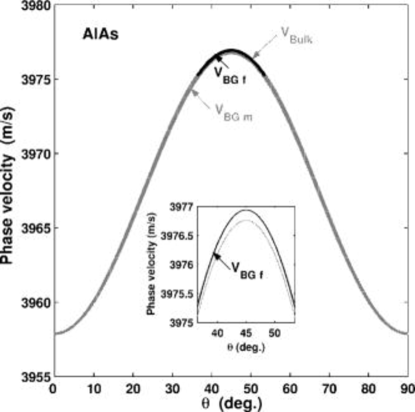
Figure 2: Speeds of piezoacoustic waves in a AlAs ($\bar{4}3$m symmetry) crystal, as a function of the cut angle: bulk shear wave (upper curve), SH surface wave for free (un-metallized) boundary conditions (intermediate curve), and SH surface wave for metallized boundary conditions (lower curve).

Note that the simple test for the solution’s validity presented in IV.B works perfectly here and henceforward. Thus using a 40 digit precision under MAPLE for AlAs, the modulus of the determinant in (42) is found to be less than 10^-19 at 45.0${}^{\circ}\pm 8.5125^{\circ}$ and more than 0.2 at $45.0^{\circ}\pm 8.5129^{\circ}$.

Figure 3 shows the variations with depth of the fields of interest (mechanical displacement, shear stress, electrical potential, electric induction) for the SH surface wave corresponding to the metallized boundary condition at $\theta=22^{\circ}30^{\prime}$. The variations of the fields are presented over 250 wavelengths, and zooms are provided for the [0, 5] wavelengths range, where $\phi$, $\sigma_{32}$, and $D_{2}$ undergo rapid changes.

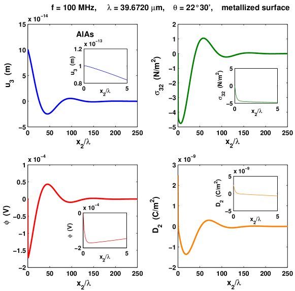
Figure 3: Depth profiles of the SH surface wave for metallized boundary conditions in a AlAs crystal cut at $22^{\circ}30^{\prime}$: mechanical displacement, shear stress, electrical potential, electric induction.

5.2 BLGO

Soluch et al.[28] measured experimentally the elastic, piezoelectric, and dielectric properties of BaLaGa₃O₇ ($\bar{4}2$m symmetry, mass density: $\rho=5450$ kg$\cdot$m^-3) as: $c_{44}=39\times 10^{9}$ N$\cdot$m^-2, $\hat{e}_{14}=0.29$ C$\cdot$m^-2, and $\epsilon_{11}=12.4\epsilon_{0}$.

Here, the speeds of the piezoacoustic SH surface wave with metallized (III.A) and with free (III.C) boundary conditions differ more notably than in the previous example from the speed of the bulk shear wave. For instance at $45^{\circ}$, these speeds are (m$\cdot$s^-1): 2700.739, 2701.239, and 2701.242, respectively. The range of values for the wave speed $v_{\text{BGm}}$ of the metallized “shorted” boundary condition is delimited above by the speed at 45^∘ and below by the speed at $0^{\circ}$ and at $90^{\circ}$, which is 2675.063 m$\cdot$s^-1. For the un-metallized “free” boundary condition, the corresponding (limited) range for the wave speed $v_{\text{BGf}}$ is bounded above by the speed at 45^∘ and below by the speed at $45.0^{\circ}\pm 7.485^{\circ}$, which is 2699.369 m$\cdot$s^-1. The difference between the two speeds is the largest at $\theta=45^{\circ}$; there the ratio $2(v_{\text{BGf}}-v_{\text{BGm}})/v_{\text{BGf}}$ is equal to 3.70 $\times 10^{-4}$.

Figure 4 displays the variations with $\theta$ of the speeds for the bulk shear wave, for the SH surface wave corresponding to the un-metallized boundary condition, and for the SH surface wave corresponding to the metallized boundary condition. Figure 5 shows the variations with depth of the fields of interest (mechanical displacement, shear stress, electrical potential, electric induction) for the SH surface wave corresponding to the metallized boundary condition at $\theta=22^{\circ}30^{\prime}$. Similar comments to those made for Figure 3 apply.

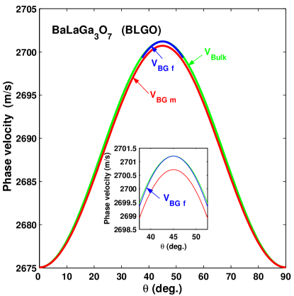
Figure 4: Speeds of piezoacoustic waves in a BaLaGa₃O₇ ($\bar{4}2$m symmetry) crystal, as a function of the cut angle: bulk shear wave (upper curve), SH surface wave for free (un-metallized) boundary conditions (intermediate curve), and SH surface wave for metallized boundary conditions (lower curve).

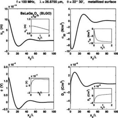
Figure 5: Depth profiles of the piezoacoustic SH surface wave for metallized boundary conditions in a BaLaGa₃O₇ crystal cut at $22^{\circ}30^{\prime}$: mechanical displacement, shear stress, electrical potential, electric induction

5.3 BGO

The relevant physical quantities of Bismuth Germanium Oxide (Bi₁₂GeO₂₀, 23 symmetry) are[29]: $\rho=9200$ kg$\cdot$m^-3, $c_{44}=25.52\times 10^{9}$ N$\cdot$m^-2, $\hat{e}_{14}=0.983$ C$\cdot$m^-2, and $\epsilon_{11}=38.0\epsilon_{0}$.

Here the differences between the speeds of the bulk shear wave, of the SH surface wave corresponding to the metallized boundary condition, and of the SH surface wave corresponding to the un-metallized boundary condition are more marked than in the previous example. At $45^{\circ}$, these speeds are (m$\cdot$s^-1): 1747.812, 1756.836, and 1756.846, respectively. At $0^{\circ}$ and at $90^{\circ}$, the speeds of the bulk shear wave and of the SH surface wave corresponding to the metallized boundary condition are both equal to 1665.507 m$\cdot$s^-1. The SH surface wave for the un-metallized boundary condition exists only in the range $45.00\pm 3.149^{\circ}$, and at the extremities of this range, its speed is 1755.068 m$\cdot$s^-1.

Figure 6 displays the variations of the three wave speeds as a function of $\theta$. Figure 7 shows the variations of the quantity $2(v_{\text{BGf}}-v_{\text{BGm}})/v_{\text{BGf}}$ with the angle of cut; its largest (smallest) value is 1.027$\times 10^{-2}$ at $45.00^{\circ}$ (0.975$\times 10^{-2}$ at $48.149^{\circ}$).

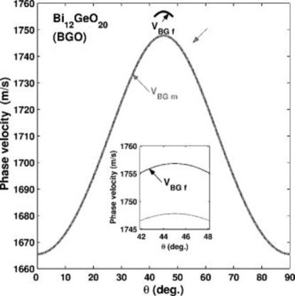
Figure 6: Speeds of piezoacoustic waves in a Bi₁₂GeO₂₀ (23 symmetry) crystal, as a function of the cut angle: bulk shear wave (upper curve), SH surface wave for free (un-metallized) boundary conditions (intermediate curve), and SH surface wave for metallized boundary conditions (lower curve).

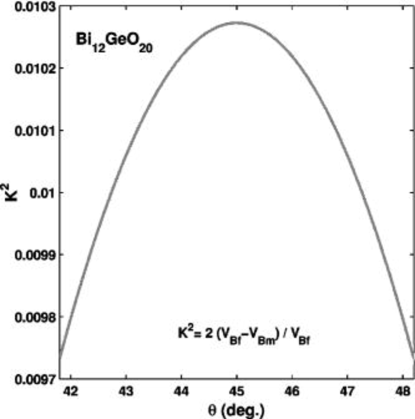
Figure 7: Variations of $2(v_{\text{BGf}}-v_{\text{BGm}})/v_{\text{BGf}}$ with $\theta$ in a Bi₁₂GeO₂₀ (23 symmetry) crystal.

Figure 8 shows the variations with depth of the fields of interest (mechanical displacement, shear stress, electrical potential, electric induction) for the SH surface wave corresponding to the metallized boundary condition at $\theta=22^{\circ}30^{\prime}$. Similar comments to those made for Figures 3 and 4 apply.

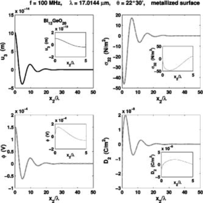
Figure 8: Depth profiles of the piezoacoustic SH surface wave for metallized boundary conditions in a Bi₁₂GeO₂₀ crystal cut at $22^{\circ}30^{\prime}$: mechanical displacement, shear stress, electrical potential, electric induction.

Figure 9 shows the variations with depth of the same fields for the SH surface wave corresponding to the un-metallized boundary condition at $\theta=42^{\circ}30^{\prime}$. By comparison with the previous Figure it can be seen that the SH surface wave for the un-metallized boundary condition penetrates far more deeply than the SH surface wave for the metallized boundary condition. The electrical potential and the electric induction are plotted inside the crystal for the range [0, 500] wavelengths, and also in the vacuum over the crystal for the range [-10, 0] wavelengths; the continuity of these fields across the interface is made apparent with a zoom for the range [-5, 5] wavelengths.

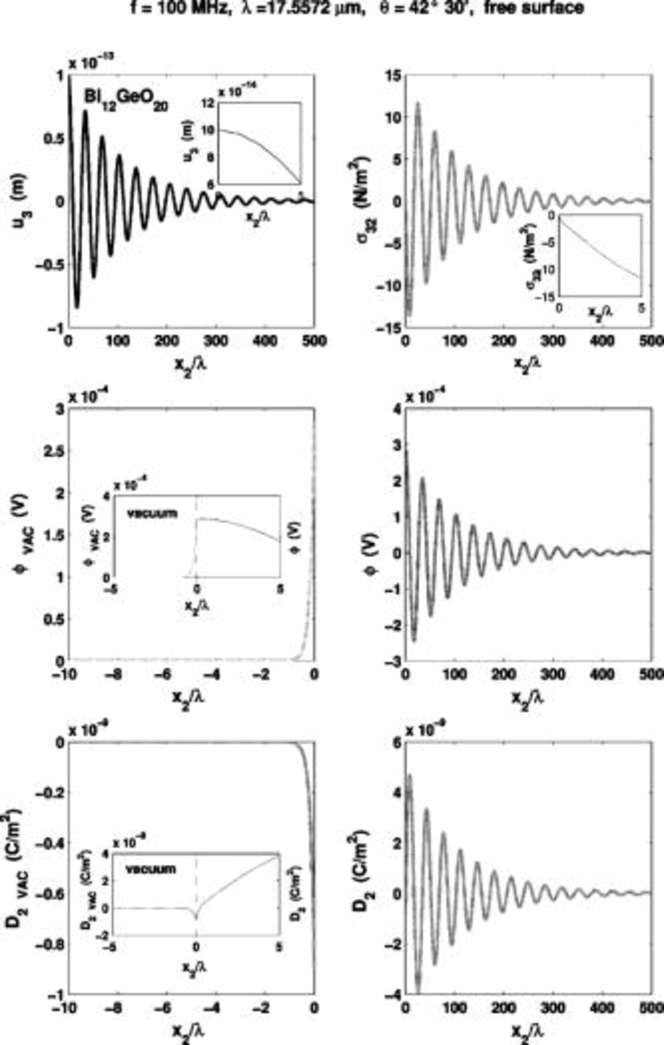
Figure 9: Depth profiles of the piezoacoustic SH surface wave for free (un-metallized) boundary conditions in a Bi₁₂GeO₂₀ crystal cut at $42^{\circ}30^{\prime}$: mechanical displacement, shear stress, electrical potential, electric induction.

6 Concluding remarks

The method of resolution for the title problem of this paper is based on the fundamental equations (15). This method has proved itself to be very effective and versatile. The end result is the complete analytical elucidation of the problem, for a great variety of surface impedance problems in a piezoelectric half-space i.e., problems where the electric induction is proportional to the electrical potential: $k\Phi=ivZD_{2}$ (say) at the boundary plane. The method can be followed through when the impedance $Z$ is zero (short-circuit), infinite (open-circuit), pure imaginary (free boundary), or complex (thin conducting layer). It has already been used for other types of surface impedance problems for elastic interface waves (Stoneley waves[20, 22], Scholte waves[21]) and could be adapted to configurations[30] with a resistance force proportional to the normal velocity, a mass concentrated in a thin surface layer, a system of elastic oscillators resting on an elastic half-space, a thin elastic layer longitudinally deformable, etc. The method can also accommodate a coupling between elastic and piezoelectric fields, in situations such as the one treated here or for instance, the case of interface acoustic waves at a domain boundary[31].

Here, attention was restricted to Bleustein-Gulyaev waves in tetragonal $\bar{4}$ piezoelectric crystals. The extension to the classes of orthorhombic 222 or monoclinic 2 crystals is straightforward and only requires the computation of the elements of the matrix $\mathbf{N}$ in Eq. (10). Their general expression is given for instance by Abbudi and Barnett[32]. As an illustration, they are now presented for rhombic 222 crystals.

For such a crystal, the relevant non-zero piezoacoustic constants in the crystallographic coordinate system are $\hat{c}_{44}$, $\hat{c}_{55}$, $\hat{e}_{14}$, $\hat{e}_{25}$, $\hat{\epsilon}_{11}$, and $\hat{\epsilon}_{22}$. In the coordinate system obtained after the rotation Eq. (1), they are

$$c_{44}=\hat{c}_{44}\cos^{2}\theta+\hat{c}_{55}\sin^{2}\theta, c_{45}=(\hat{c}_{44}-\hat{c}_{55})\cos\theta\sin\theta,$$

$$c_{55}=\hat{c}_{55}\cos^{2}\theta+\hat{c}_{44}\sin^{2}\theta, \epsilon_{12}=(\hat{\epsilon}_{22}-\hat{\epsilon}_{11})\cos\theta\sin\theta,$$

$$\epsilon_{11}=\hat{\epsilon}_{11}\cos^{2}\theta+\hat{\epsilon}_{22}\sin^{2}\theta, \epsilon_{22}=\hat{\epsilon}_{22}\cos^{2}\theta+\hat{\epsilon}_{11}\sin^{2}\theta,$$

$$e_{14}=\hat{e}_{14}\cos^{2}\theta-\hat{e}_{25}\sin^{2}\theta, e_{15}=(\hat{e}_{14}+\hat{e}_{25})\cos\theta\sin\theta,$$

$$e_{25}=\hat{e}_{25}\cos^{2}\theta-\hat{e}_{14}\sin^{2}\theta, e_{24}=-\hat{e}_{15}.$$ (44)

The equations of motion can be cast in the form Eq. (10) where the matrix $\mathbf{N}$ is defined by its $2\times 2$ blocks $\mathbf{N^{(1)}_{1}}$, $\mathbf{N^{(1)}_{2}}$, $\mathbf{K^{(1)}}$ in Eq. (11). The components of $-\mathbf{N^{(1)}_{1}}$ and $\mathbf{N^{(1)}_{2}}$ are given here by

$$\begin{bmatrix}\left(\dfrac{\epsilon_{22}c_{45}}{e_{14}e_{15}}-\dfrac{e_{25}}{e_{14}}\right)\kappa^{2}&\left(\dfrac{\epsilon_{22}}{e_{15}}+\dfrac{\epsilon_{12}}{e_{14}}\right)\kappa^{2}\vspace{8pt}\\ -\left(\dfrac{c_{44}e_{25}}{e_{14}e_{15}}+\dfrac{c_{45}}{e_{14}}\right)\kappa^{2}&\left(\dfrac{\epsilon_{12}c_{44}}{e_{14}e_{15}}-1\right)\kappa^{2}\end{bmatrix},\quad\begin{bmatrix}\dfrac{\epsilon_{22}}{e_{14}e_{15}}\kappa^{2}&-\dfrac{1}{e_{14}}\kappa^{2}\vspace{8pt}\\ -\dfrac{1}{e_{14}}\kappa^{2}&-\dfrac{c_{44}}{e_{14}e_{15}}\kappa^{2}\end{bmatrix},$$ (45)

respectively, and those of $\mathbf{K^{(1)}}$ are

$$K^{(1)}_{11}=X-c_{55}-\left(c_{44}\dfrac{e_{25}^{2}}{e_{14}e_{15}}+2c_{45}\dfrac{e_{25}}{e_{14}}-c_{45}\dfrac{\epsilon_{22}c_{45}}{e_{14}e_{15}}\right)\kappa^{2},$$

$$K^{(1)}_{12}=-e_{15}+\left[\dfrac{c_{44}\epsilon_{12}}{e_{14}}+\dfrac{c_{45}\epsilon_{22}}{e_{15}}+e_{25}\left(\dfrac{\epsilon_{12}c_{44}}{e_{14}e_{15}}-1\right)\right]\kappa^{2},$$

$$K^{(1)}_{22}=-\epsilon_{11}+\left[\epsilon_{12}\left(\dfrac{\epsilon_{12}c_{44}}{e_{14}e_{15}}-2\right)-\epsilon_{22}\dfrac{e_{14}}{e_{15}}\right]\kappa^{2}.$$ (46)

Here, the quantity $\kappa^{2}$ is defined by

$$\kappa^{2}=\dfrac{e_{14}e_{15}}{\epsilon_{11}c_{44}+e_{15}^{2}}.$$ (47)

Finally, in guise of a Conclusion, the main relevant advances toward the full resolution of the problem presented in the paper are recapitulated. In the purely elastic case, the secular equation for Rayleigh waves polarized in a plane of symmetry was derived by Currie[33] who, using an algebraic approach based on the Stroh formalism, obtained the equations,

$$\overline{\mathbf{U}}(0)\cdot\mathbf{K^{(n)}}\mathbf{U}(0)=0,$$ (48)

where $\mathbf{U}(0)$ is the mechanical displacement on the free surface. Although these equations are also valid in generally anisotropic crystals, his derivation of the secular equation for triclinic (no symmetry) crystals apparently leads to a trivial identity. This problem was later corrected by Taylor and Currie[34] and by Taziev[35] (see also Ting[36]). In contrast to these approaches based on the formulation of the equations of motion as a first-order differential system for the displacement-traction vector, Mozhaev[37] wrote the equations of motion as a second-order differential system for the displacement vector,

$$\mathbf{\alpha U}^{\prime\prime}-i\mathbf{\beta U}^{\prime}+\mathbf{\gamma U}=\mathbf{0},$$ (49)

where $\mathbf{\alpha}$, $\mathbf{\beta}$, $\mathbf{\gamma}$, are real symmetric matrices. Then, using first integrals, he quickly derived the secular equation for orthorhombic crystals. Destrade[38] rewrote the equations of motion, this time in the form

$$\mathbf{\hat{\alpha}t}^{\prime\prime}-i\mathbf{\hat{\beta}t}^{\prime}+\mathbf{\hat{\gamma}t}=\mathbf{0},$$ (50)

for the tractions, where $\mathbf{\hat{\alpha}}$, $\mathbf{\hat{\beta}}$, $\mathbf{\hat{\gamma}}$, are real symmetric matrices. Adapting Mozhaev’s first integrals, he re-derived (unaware of Currie’s result) the secular equation for Rayleigh waves polarized in a symmetry plane. He also mentioned (and the proof was later given in the review article by Ting[39]) that the method of first integrals could not be used for arbitrary anisotropy when the equations of motion are written as Eq. (49) or Eq. (50). Recently[20, 21, 22] he made the connection between Currie’s and Taziev’s use of integer powers of the Stroh matrix $\mathbf{N}$ and Mozhaev’s first integrals, as shown also here in II.C. Note that Mozhaev and Weihnacht[15] were able to solve the problem of SH surface modes of a 2mm crystal using first integrals of the piezoacoustic equations written as a second-order differential system.

References

- [1] J. L. Bleustein, “A new surface wave in piezoelectric materials”, Appl. Phys. Lett. 13, 412–413 (1968).
- [2] Yu. V. Gulyaev, “Electroacoustic surface waves in piezoelectric materials”, JETP Lett. 9, 37–38 (1969).
- [3] C. -C. Tseng, “Piezoelectric surface waves in cubic crystals”, J. Appl. Phys. 41, 2270–2276 (1970).
- [4] K. Nakamura and M. Oshiki, “Theoretical analysis of horizontal shear mode piezoelectric surface acoustic waves in potassium niobate”, Appl. Phys. Lett. 71, 3203–3205 (1997).
- [5] M. Kadota, T. Yoneda, K. Fujimoto, T. Nakao, and E. Takata, “Very small-sized resonator IF filter using shear horizontal wave on quartz substrate”, IEEE Ultrason. Symp. Proc. 1, 65–68 (2001).
- [6] M. Kadota, J. Ago, H. Horiuchi, and M. Ikeura, “Longitudinally coupled resonator filter using edge reflection of Bleustein-Gulyaev-Shimizu and shear horizontal waves with various bandwidths realized by selecting substrates”, Jpn. J. Appl. Phys. 1 40, 3722–3725 (2001).
- [7] G. Koerber and R. F. Vogel, “Generalized Bleustein modes”, IEEE Trans. Sonics Ultrason. SU-19, 3–8 (1972).
- [8] G. G. Koerber and R. F. Vogel, “SH-mode piezoelectric surface waves on rotated cuts”, IEEE Trans. Sonics Ultrason. SU-20, 10–12 (1973).
- [9] L. S. Braginskiĭ and I. A. Gilinskiĭ, “Generalized shear surface waves in piezoelectric crystals”, Sov. Phys. Solid State 21, 2035–2037 (1979).
- [10] E. L. Alburque and N. C. Chao, “On the propagation of elastic surface waves in piezoelectric crystals”, Phys. Status Sol. B 104, K11–K14 (1981).
- [11] V. R. Velasco, “Surface and interface Bleustein-Gulyaev waves along symmetry directions of cubic crystals”, Surf. Sci. 139, 63–74 (1984).
- [12] Yu. A. Kosevich and E. S. Syrkin, “Generalized surface shear waves in piezoelectric crystals”, Sov. Phys. Solid State 28, 134–139 (1986).
- [13] V. M. Bright and W. D. Hunt, “Bleustein-Gulyaev waves in Gallium Arsenide and other piezoelectric cubic crystals”, J. Appl. Phys. 66, 1556–1564 (1989).
- [14] G. G. Kessenikh and L. A. Shuvalov, “Bleustein-Gulyaev surface waves in monoclinic piezoelectric crystals”, Sov.Phys. Cryst. 21, 1–3 (1976).
- [15] V. G. Mozhaev and M. Weihnacht, “Sectors of nonexistence of surface acoustic waves in potassium niobate”, IEEE Ultras. Symp. Proc. 1, 391–395 (2002).
- [16] G. W. Farnell and E. L. Adler, in Physical Acoustics, Vol. 9, edited by W.P. Mason and R.N. Thurston, Academic Press, New York (1972) 35–127.
- [17] E. A. Kraut, “New mathematical formulation for piezoelectric wave propagation”, Phys. Rev. 188, 1450–1455 (1969).
- [18] A. N. Stroh, “Dislocations and cracks in anisotropic elasticity,” Phil. Mag. 3, 625–646 (1958).
- [19] A. H. Fahmy and E. L. Adler, “Propagation of acoustic surface waves in multilayers: A matrix description”, Appl. Phys. Lett. 22, 495–497 (1973).
- [20] M. Destrade, “Elastic interface acoustic waves in twinned crystals”, Int. J. Solids Struct. 40, 7375–7383 (2003) .
- [21] M. Destrade, “Explicit secular equation for Scholte waves over a monoclinic crystal”, J. Sound Vibr. 273, 409–414 (2004).
- [22] M. Destrade, “On interface waves in misoriented pre-stressed incompressible elastic solids”, IMA J. Appl. Math. (to appear).
- [23] K. A. Ingebrigsten, “Surface waves in piezoelectric”, J. Appl. Phys. 40, 2681–2686 (1969).
- [24] J. Lothe and D. M. Barnett, “Integral formalism for surface waves in piezoelectric crystals. Existence considerations”, J. Appl. Phys. 47, 1799–1807 (1976).
- [25] E. Dieulesaint and D. Royer, Elastic waves in solids. Applications to signal processing. (John Wiley, 1980).
- [26] D. Royer et E. Dieulesaint, Ondes élastiques dans les solides. I. Propagation libre et guidée (Elastic waves in solids. Free and guided propagation.) (Masson, 1996).
- [27] Y. Kim and W. D. Hunt, “Acoustic fields and velocities for surface-acoustic-wave propagation in multilayered structures: An extension of the Laguerre polynomial approach”, J. Appl. Phys. 68, 4993–4997 (1990).
- [28] W. Soluch, R. Ksiezopolski, W. Piekarczyk, M. Berkowski, M. A. Goodberlet, and J. F. Vetelino, “Elastic, piezoelectric, and dielectric properties of the BaLaGa3O7 crystal”, J. Appl. Phys. 58, 2285–2287 (1985).
- [29] B. A. Auld, Acoustic fields and waves in solids. (Wiley, 1973).
- [30] S. Kaliski, “On the existence of transversal surface waves in an elastic half-space with surface impedance”, Bull. Acad. Polon. Sci., Sér. sci. techn. 15, 467–472 (1967).
- [31] V.G. Mozhaev, M. Weihnacht, “Interface acoustic waves at a 180 degrees domain boundary in tetragonal barium titanate”, J. Kor. Phys. Soc. 32, S747–S749 (1998).
- [32] M. Abbudi and D. M. Barnett, “On the existence of interfacial (Stoneley) waves in bonded piezoelectric half-spaces”, Proc. Roy. Soc. London A 429, 587–611 (1990).
- [33] P. K. Currie, “The secular equation for Rayleigh waves on elastic crystals”, Quart. J. Mech. appl. Math. 32, 163–173 (1979).
- [34] D. B. Taylor and P. K. Currie, “The secular equation for Rayleigh waves on elastic crystals II: Corrections and additions”, Quart. J. Mech. appl. Math. 34, 231–234 (1981).
- [35] R. M. Taziev, “Dispersion relation for acoustic waves in an anisotropic elastic half-space”, Sov. Phys. Acoust. 35, 535–538 (1989).
- [36] T. C. T. Ting, “The polarization vector and secular equation for surface waves in an anisotropic elastic half-space”, Int. J. Solids Struct. 41, 2065–2083 (2004).
- [37] V. G. Mozhaev, “Some new ideas in the theory of surface acoustic waves in anisotropic media,” IUTAM Symposium on anisotropy, inhomogeneity and nonlinearity in solids (D.F. Parker and A.H. England, eds.), 455–462 (Kluwer, 1995).
- [38] M. Destrade, “The explicit secular equation for surface acoustic waves in monoclinic elastic crystals”, J. Acoust. Soc. Am. 109, 1398-1402 (2001).
- [39] T. C. T. Ting, “Explicit secular equations for surface waves in an anisotropic elastic half-space: from Rayleigh to today”, In Proc. NATO Adv. Res. Workshop on Surface Waves in Anisotropic and Laminated Bodies and Defects Detection, Moscow, Russia, 7-9 February 2002; (G. A. Maugin and R. V. Goldstein, eds.; Kluwer, 2004).