Minimal Residual Methods for Complex Symmetric, Skew Symmetric, and Skew Hermitian Systems

Abstract

While there is no lack of efficient Krylov subspace solvers for Hermitian systems, few exist for complex symmetric, skew symmetric, or skew Hermitian systems, which are increasingly important in modern applications including quantum dynamics, electromagnetics, and power systems. For a large, consistent, complex symmetric system, one may apply a non-Hermitian Krylov subspace method disregarding the symmetry of $A$, or a Hermitian Krylov solver on the equivalent normal equation or an augmented system twice the original dimension. These have the disadvantages of increasing memory, conditioning, or computational costs. An exception is a special version of QMR by Freund (1992), but that may be affected by nonbenign breakdowns unless look-ahead is implemented; furthermore, it is designed for only consistent and nonsingular problems. Greif and Varah (2009) adapted CG for nonsingular skew symmetric linear systems that are necessarily and restrictively of even order.

We extend the symmetric and Hermitian algorithms MINRES and MINRES-QLP by Choi, Paige, and Saunders (2011) to complex symmetric, skew symmetric, and skew Hermitian systems. In particular, MINRES-QLP uses a rank-revealing QLP decomposition of the tridiagonal matrix from a three-term recurrent complex symmetric Lanczos process. Whether the systems are real or complex, singular or invertible, compatible or inconsistent, MINRES-QLP computes the unique minimum-length (i.e., pseudoinverse) solutions. It is a significant extension of MINRES by Paige and Saunders (1975) with enhanced stability and capability.

Dedicated to Michael Saunders’s 70th birthday

xxx/xxxxxxxxx

1 Introduction

Krylov subspace methods for linear systems are generally divided into two classes: those for Hermitian matrices (e.g., CG [27], MINRES [38], SYMMLQ [38], MINRES-QLP [9, 13, 11, 6]) and those for general matrices without such symmetries (e.g., BiCG [16], GMRES [41], QMR [20], BiCGstab [53], LSQR [39, 40], and IDR$(s)$ [45]). Such a division is largely due to historical reasons in numerical linear algebra—the most prevalent structure for matrices arising from practical applications being Hermitian (which reduces to symmetric for real matrices). However, other types of symmetry structures, notably complex symmetric, skew symmetric, and skew Hermitian matrices, are becoming increasingly common in modern applications. Currently, except possibly for storage and matrix-vector products, these are treated as general matrices with no symmetry structures. The algorithms in this article go substantially further in developing specialized Krylov subspace algorithms designed at the outset to exploit the symmetry structures. In addition, our algorithms constructively reveal the (numerical) compatibility and singularity of a given linear system; users do not have to know these properties a priori.

We are concerned with iterative methods for solving a large linear system $Ax=b$ or the more general minimum-length least-squares (LS) problem

$$\min\|x\|_{2}\quad\text{s.t.}\quad x\in\arg\min_{x\in\mathbb{C}^{n}}\|Ax-b\|_{2},$$ (1)

where $A\in\mathbb{C}^{n\times n}$ is complex symmetric ($A=A^{T}\!$ ) or skew Hermitian ($A=-A^{*}$), and possibly singular, and $b\in\mathbb{C}^{n}$. Our results are directly applicable to problems with symmetric or skew symmetric matrices $A=\pm A^{T}\!\in\mathbb{R}^{n\times n}$ and real vectors $b$. $A$ may exist only as an operator for returning the product $Ax$.

The solution of (1), called the minimum-length or pseudoinverse solution [22], is formally given by $x^{\dagger}=(A^{*}A)^{\dagger}A^{*}b$, where $A^{\dagger}$ denotes the pseudoinverse of $A$. The pseudoinverse is continuous under perturbations $E$ for which $\mathop{\operator@font rank}\nolimits{(A+E)}=\mathop{\operator@font rank}\nolimits{(A)}$ [47], and $x^{\dagger}$ is continuous under the same condition. Problem (1) is then well-posed [24].

Let $A=U\Sigma U^{T}\!$ be a Takagi decomposition [29], a singular-value decomposition (SVD) specialized for a complex symmetric matrix, with $U$ unitary ($U^{*}U=I$) and $\Sigma\equiv\mathop{\operator@font diag}\nolimits({\left[\begin{smallmatrix}\sigma_{1},\ldots,\sigma_{n}\end{smallmatrix}\right]})$ real non-negative and $\sigma_{1}\geq\sigma_{2}\geq\cdots\geq\sigma_{r}>0$, where $r$ is the rank of $A$. We define the condition number of $A$ to be $\kappa(A)=\smash[b]{\frac{\sigma_{1}}{\sigma_{r}}}$, and we say that $A$ is ill-conditioned if $\kappa(A)\gg 1$. Hence a mathematically nonsingular matrix (e.g., $A={\left[\begin{smallmatrix}1&0\\ 0&\varepsilon\end{smallmatrix}\right]}$, where $\varepsilon$ is the machine precision) could be regarded as numerically singular. Also, a singular matrix could be well-conditioned or ill-conditioned. For a skew Hermitian matrix, we use its (full) eigenvalue decomposition $A=V\Lambda V^{*}$, where $\Lambda$ is a diagonal matrix of imaginary numbers (possibly zeros; in conjugate pairs if $A$ is real, i.e., skew symmetric) and $V$ is unitary. We define its condition number as $\kappa(A)=\smash[b]{\frac{|\lambda_{1}|}{|\lambda_{r}|}}$, the ratio of the largest and smallest nonzero eigenvalues in magnitude.

Example 1.1.

We contrast the five classes of symmetric or Hermitian matrices by their definitions and small instances of order $n=2$:

$$\mathbb{R}^{n\times n}\ni A =A^{T}\!={\begin{bmatrix}1&5\\ 5&1\end{bmatrix}}\text{ is symmetric}.$$

$$\mathbb{C}^{n\times n}\ni A =A^{*}={\begin{bmatrix}1&1-2i\\ 1+2i&1\end{bmatrix}}\text{ is Hermitian (with real diagonal)}.$$

$$\mathbb{C}^{n\times n}\ni A =A^{T}\!={\begin{bmatrix}2+i&1-2i\\ 1-2i&i\end{bmatrix}}\text{ is complex symmetric (with complex diagonal)}.$$

$$\mathbb{R}^{n\times n}\ni A =-A^{T}\!={\begin{bmatrix}0&5\\ -5&0\end{bmatrix}}\text{ is skew symmetric (with zero diagonal)}.$$

$$\mathbb{C}^{n\times n}\ni A =-A^{*}={\begin{bmatrix}0&1-2i\\ -1-2i&{\color[rgb]{0,0,0}\hbox{}i}\end{bmatrix}}\text{ is skew Hermitian (with {\color[rgb]{0,0,0}\hbox{}imaginary} diagonal)}.$$

CG, SYMMLQ, and MINRES are designed for solving nonsingular symmetric systems $Ax=b$. CG is efficient on symmetric positive definite systems. For indefinite problems, SYMMLQ and MINRES are reliable even if $A$ is ill-conditioned.

Choi [6] appears to be the first to comparatively analyze the algorithms on singular symmetric and Hermitian problems. On (singular) incompatible problems CG and SYMMLQ iterates $x_{k}$ diverge to some nullvectors of $A$ [6, Propositions 2.7, 2.8, and 2.15; Lemma 2.17]. MINRES often seems more desirable to users because its residual norms are monotonically decreasing. On singular compatible systems, MINRES returns $x^{\dagger}$ [6, Theorem 2.25]. On singular incompatible systems, MINRES remains reliable if it is terminated with a suitable stopping rule that monitors $\|Ar_{k}\|$ [9, Lemma 3.3], but the solution is generally not $x^{\dagger}$ [9, Theorem 3.2]. MINRES-QLP [9, 13, 11, 6] is a significant extension of MINRES, capable of computing $x^{\dagger}$, simultaneously minimizing residual and solution norms. The additional cost of MINRES-QLP is moderate relative to MINRES: $1$ vector in memory, $4$ axpy operations ($y\leftarrow\alpha x+y$), and $3$ vector scalings ($x\leftarrow\alpha x$) per iteration. The efficiency of MINRES is partially, and in some cases almost fully, retained in MINRES-QLP by transferring from a MINRES phase to a MINRES-QLP phase only when an estimated $\kappa(A)$ exceeds a user-specified value. The MINRES phase is optional, consisting of only MINRES iterations for nonsingular and well-conditioned subproblems. The MINRES-QLP phase handles less well-conditioned and possibly numerically singular subproblems. In all iterations, MINRES-QLP uses QR factors of the tridiagonal matrix from a Lanczos process and then applies a second QR decomposition on the conjugate transpose of the upper-triangular factor to obtain and reveal the rank of a lower-tridiagonal form. On nonsingular systems, MINRES-QLP enhances the accuracy (with smaller rounding errors) and stability of MINRES. It is applicable to symmetric and Hermitian problems with no traditional restrictions such as nonsingularity and definiteness of $A$ or compatibility of $b$.

The aforementioned established Hermitian methods are not, however, directly applicable to complex or skew symmetric equations. For consistent complex symmetric problems, which could arise in Helmholtz equations, linear systems that involve Hankel matrices, or applications in quantum dynamics, electromagnetics, and power systems, we may apply a non-Hermitian Krylov subspace method disregarding the symmetry of $A$ or a Hermitian Krylov solver (such as CG, SYMMLQ, MINRES, or MINRES-QLP) on the equivalent normal equation or an augmented system twice the original dimension. They suffer increasing memory, conditioning, or computational costs. An exception is a special version of QMR by Freund (1992) [19], which takes advantage of the matrix symmetry by using an unsymmetric Lanczos framework. Unfortunately, the algorithm may be affected by nonbenign breakdowns unless a look-ahead strategy is implemented. Another less than elegant feature of QMR is that the vector norm of choice is induced by the inner product $x^{T}\!y$ but it is not a proper vector norm (e.g., $0\neq x^{T}\!:={\left[\begin{smallmatrix}1&i\end{smallmatrix}\right]}$, where $i=\sqrt{-1}$, yet $x^{T}\!x=0$). Besides, QMR is designed for only nonsingular and consistent problems. Inconsistent complex symmetric problems (1) could arise from shifted problems in inverse or Rayleigh quotient iterations; mathematically or numerically singular or inconsistent systems, in which $A$ or $b$ are vulnerable to errors due to measurement, discretization, truncation, or round-off. In fact, QMR and most non-Hermitian Krylov solvers (other than LSQR) fail to converge to $x^{\dagger}$ on an example as simple as $A=i\;\mathop{\operator@font diag}\nolimits({\left[\begin{smallmatrix}1\\ 0\end{smallmatrix}\right]})$ and $b=i{\left[\begin{smallmatrix}1\\ 1\end{smallmatrix}\right]}$, for which $x^{\dagger}={\left[\begin{smallmatrix}1\\ 0\end{smallmatrix}\right]}$.

Here we extend the symmetric and Hermitian algorithms MINRES and MINRES-QLP The main aim is to deal reliably with compatible or incompatible systems and to return the unique solution of (1). Like QMR and the Hermitian Krylov solvers, our approach exploits the matrix symmetry.

Noting the similarities in the definitions of skew symmetric matrices ($A=-A^{T}\!\in\mathbb{R}^{n\times n}$) and complex symmetric matrices and motivated by algebraic Riccati equations [32] and more recent, novel applications of Hodge theory in data mining [33, 21], we evolve MINRES-QLP further for solving skew symmetric linear systems. Greif and Varah [23] adapted CG for nonsingular skew symmetric linear systems that are skew-$A$ conjugate, meaning $-A^{2}$ is symmetric positive definite. The algorithm is further restricted to $A$ of even order because a skew symmetric matrix of odd order is singular. Our MINRES-QLP extension has no such limitations and is applicable to singular problems. For skew Hermitian systems with skew Hermitian matrices or operators ($A=-A^{*}\in\mathbb{C}^{n\times n}$), our approach is to transform them into Hermitian systems so that they can immediately take advantage of the original Hermitian version of MINRES-QLP.

1.1 Notation

For an incompatible system, $Ax\approx b$ is shorthand for the LS problem (1). We use “$\simeq$” to mean “approximately equal to.” The letters $i$, $j$, $k$ in subscripts or superscripts denote integer indices; $i$ may also represent $\sqrt{-1}$. We use $c$ and $s$ for cosine and sine of some angle $\theta$; $e_{k}$ is the $k$th unit vector; $e$ is a vector of all ones; and other lower-case letters such as $b$, $u$, and $x$ (possibly with integer subscripts) denote column vectors. Upper-case letters $A$, $T_{k}$, $V_{k}$, … denote matrices, and $I_{k}$ is the identity matrix of order $k$. Lower-case Greek letters denote scalars; in particular, $\varepsilon\simeq 10^{-16}$ denotes floating-point double precision. If a quantity $\delta_{k}$ is modified one or more times, we denote its values by $\delta_{k}$, $\delta_{k}^{(2)}$, and so on. We use $\mathop{\operator@font diag}\nolimits(v)$ to denote a diagonal matrix with elements of a vector $v$ on the diagonal. The transpose, conjugate, and conjugate transpose of a matrix $A$ are denoted by $A^{T}\!$, $\overline{A}$, and $A^{*}=\overline{A}^{T}\!$, respectively. The symbol $\|\,\cdot\,\|$ denotes the $2$-norm of a vector ($\|x\|=\sqrt{x^{*}x}$) or a matrix ($\|A\|=\sigma_{1}$ from $A$’s SVD).

1.2 Overview

In Section 2 we briefly review the Lanczos processes and QLP decomposition before developing the algorithms in Sections 3-5. Preconditioned algorithms are described in Section 6. Numerical experiments are described in Section 7. We conclude with future work and related software in Section 8. Our pseudocode and a summary of norm estimates and stopping conditions are given in Appendices A and B.

2 Review

In the following few subsections, we summarize algebraic methods necessary for our algorithmic development.

2.1 Saunders and Lanczos processes

Given a complex symmetric operator $A$ and a vector $b$, a Lanczos-like process [2], which we name the Saunders process, computes vectors $v_{k}$ and tridiagonal matrices $\underline{T_{k}}$ according to $v_{0}\equiv 0$, $\beta_{1}v_{1}=b$, and then

$$p_{k}=A\overline{v}_{k},\qquad\alpha_{k}=v_{k}^{*}p_{k},\qquad\beta_{k+1}v_{k+1}=p_{k}-\alpha_{k}v_{k}-\beta_{k}v_{k-1}$$ (2)

for $k=1,2,\dots,\ell$, where we choose $\beta_{k}>0$ to give $\|v_{k}\|=1$. In matrix form,

$$A\overline{V}\!_{k}\!=\!V_{k+1}\underline{T_{k}},\quad\underline{T_{k}}\!\equiv\!\mbox{\footnotesize${\begin{bmatrix}\alpha_{1}&\beta_{2}\\ \beta_{2}&\alpha_{2}&\ddots\\ &\ddots&\ddots&\beta_{k}\\ &&\beta_{k}&\alpha_{k}\\ &&&\beta_{k+1}\end{bmatrix}}$}\!\equiv\!{\begin{bmatrix}T_{k}\\ \beta_{k+1}e_{k}^{T}\end{bmatrix}},\quad V_{k}\!\equiv\!{\begin{bmatrix}v_{1}&\!\cdots\!&v_{k}\end{bmatrix}}.$$ (3)

In exact arithmetic, the columns of $V_{k}$ are orthogonal, and the process stops with $k=\ell$ and $\beta_{\ell+1}=0$ for some $\ell\leq n$, and then $A\overline{V}\!_{\ell}=V_{\ell}T_{\ell}$. For derivation purposes we assume that this happens, though in practice it is rare unless $V_{k}$ is reorthogonalized for each $k$. In any case, (3) holds to machine precision, and the computed vectors satisfy $\|V_{k}\|_{1}\simeq 1$ (even if $k\gg n$).

If instead we are given a skew symmetric $A$, the following is a Lanczos process [23, Algorithm 1] that transforms $A$ to a series of expanding, skew symmetric tridiagonal matrices $T_{k}$ and generates a set of orthogonal vectors in $V_{k}$ in exact arithmetic:

$$p_{k}=Av_{k},\qquad-\beta_{k+1}v_{k+1}=p_{k}-\beta_{k}v_{k-1}{\color[rgb]{0,0,0}\hbox{},}$$ (4)

where $\beta_{k}>0$ for $k<\ell$. Its associated matrix form is

$$AV_{k}\!=\!V_{k+1}\underline{T_{k}},\quad\underline{T_{k}}\!\equiv\!\mbox{\footnotesize${\begin{bmatrix}0&\beta_{2}\\ -{\beta}_{2}&0&\ddots\\ &\ddots&\ddots&\beta_{k}\\ &&-{\beta}_{k}&0\\ &&&-{\beta}_{k+1}\end{bmatrix}}$}\!\equiv\!{\begin{bmatrix}T_{k}\\ -\beta_{k+1}e_{k}^{T}\end{bmatrix}}.$$ (5)

If the skew symmetric process were forced on a skew Hermitian matrix, the resultant $V_{k}$ would not be orthogonal. Instead, we multiply $Ax\approx b$ by $i$ on both sides to yield a Hermitian problem since $(iA)^{*}=\overline{i}A^{*}=iA$. This simple transformation by a scalar multiplication preserves the conditioning since $\kappa(A)=\kappa(iA)$ and allows us to adapt the original Hermitian Lanczos process with $v_{0}\equiv 0$, $\beta_{1}v_{1}=ib$, followed by

$$p_{k}=iAv_{k},\qquad\alpha_{k}=v_{k}^{*}p_{k},\qquad\beta_{k+1}v_{k+1}=p_{k}-\alpha_{k}v_{k}-\beta_{k}v_{k-1}.$$ (6)

Its matrix form is the same as (3) except that the first equation is $iAV_{k}=V_{k+1}\underline{T_{k}}$.

2.2 Properties of the Lanczos processes

The following properties of the Lanczos processes are notable:

1. If $A$ and $b$ are real, then the Saunders process (2) for a complex symmetric system reduces to the symmetric Lanczos process.

2. The complex and skew symmetric properties of $A$ carry over to $T_{k}$ by the Lanczos processes (2) and (4), respectively. From the skew Hermitian process (6), $T_{k}$ is symmetric.

3. The skew symmetric Lanczos process (4) is only two-term recurrent.

4. In (6), there are two ways to form $p_{k}$: $p_{k}=(iA)v_{k}$ or $p_{k}=A(iv_{k})$. One may be cheaper than the other. If $A$ is dense, $iA$ takes $\mathcal{O}(n^{2})$ scalar multiplications and storage. If $A$ is sparse or structured as in the case of Toeplitz, $iA$ just takes $\mathcal{O}(n)$ multiplications. In contrast, $iv_{k}$ takes $n{\color[rgb]{0,0,0}\hbox{}\wp}$ multiplications, where ${\color[rgb]{0,0,0}\hbox{}\wp}$ is theoretically bounded by the number of distinct nonzero eigenvalues of $A$; but in practice ${\color[rgb]{0,0,0}\hbox{}\wp}$ could be an integer multiple of $n$.

5. While the skew Hermitian Lanczos process (6) is applicable to a skew symmetric problem, it involves complex arithmetic and is thus computationally more costly than the skew symmetric Lanczos process with a real vector $b$.

6. If $A$ is changed to $A-\sigma I$ for some scalar shift $\sigma$, then $T_{k}$ becomes $T_{k}-\sigma I$, and $V_{k}$ is unaltered, showing that singular systems are commonplace. Shifted problems appear in inverse iteration or Rayleigh quotient iteration. The Saunders and Lanczos frameworks efficiently handle shifted problems.

7. Shifted skew symmetric matrices are not skew symmetric. This notion also applies to the case of shifted skew Hermitian matrices. Nevertheless they arise often in Toeplitz problems [3, 4].

8. For the skew Lanczos processes, the $k$th Krylov subspace generated by $A$ and $b$ is defined to be $\mathcal{K}_{k}(A,b)=\mathop{\mathrm{range}}(V_{k})=\mbox{\rm span}\{b,Ab,\dots,A^{k-1}b\}$. For the Saunders process, we have a modified Krylov subspace [43] that we call the Saunders subspace, $\mathcal{S}_{k}(A,b)\equiv\mathcal{K}_{k_{1}}(A\overline{A},b)\oplus\mathcal{K}_{k_{2}}(A\overline{A},A\overline{b})$, where $\oplus$ is the direct-sum operator, $k_{1}+k_{2}=k$, and $0\leq k_{1}-k_{2}\leq 1$.

9. $\underline{T_{k}}$ has full column rank $k$ for all $k<\ell$ because $\beta_{1},\dots,\beta_{k+1}>0$.

Theorem 1.

$T_{\ell}$ is nonsingular if and only if $b\in\mathop{\mathrm{range}}(A)$. Furthermore, $\mathop{\operator@font rank}\nolimits(T_{\ell})=\ell-1$ in the case $b\notin\mathop{\mathrm{range}}(A)$.

Proof.

We prove below for $A$ complex symmetric. The proofs are similar for the skew symmetric and skew Hermitian cases.

We use $A\overline{V}_{\ell}=V_{\ell}T_{\ell}$ twice. First, if $T_{\ell}$ is nonsingular, we can solve $T_{\ell}y_{\ell}=\beta_{1}e_{1}$ and then $A\overline{V}_{\ell}y_{\ell}=V_{\ell}T_{\ell}y_{\ell}=V_{\ell}\beta_{1}e_{1}=b$. Conversely, if $b\in\mathop{\mathrm{range}}(A)$, then $\mathop{\mathrm{range}}(\overline{V}_{\ell})\subseteq\mathop{\mathrm{range}}(\overline{A})=\mathop{\mathrm{range}}(A^{*})$. Suppose $T_{\ell}$ is singular. Then there exists $z\neq 0$ such that $T_{\ell}z=0$ and thus $V_{\ell}T_{\ell}z=A\overline{V}_{\ell}z=0$. That is, $0\neq\overline{V}_{\ell}z\in\mathop{\mathrm{null}}(A)$. But this is impossible because $\overline{V}_{\ell}z\in\mathop{\mathrm{range}}(A^{*})$ and $\mathop{\mathrm{null}}(A)\cap\mathop{\mathrm{range}}(A^{*})=\{0\}$. Thus $T_{\ell}$ must be nonsingular.

If $b\notin\mathop{\mathrm{range}}(A)$, $T_{\ell}={\begin{bmatrix}\underline{T_{\ell-1}}&\begin{smallmatrix}\beta_{\ell}e_{\ell-1}\\ \alpha_{\ell}\end{smallmatrix}\end{bmatrix}}$ is singular. It follows that $\ell>\mathop{\operator@font rank}\nolimits(T_{\ell})\geq\mathop{\operator@font rank}\nolimits(\underline{T_{\ell-1}})=\ell-1$ since $\mathop{\operator@font rank}\nolimits(\underline{T_{k}})=k$ for all $k<\ell$. Therefore $\mathop{\operator@font rank}\nolimits(T_{\ell})=\ell-1$. ∎

2.3 QLP decompositions for singular matrices

Here we generalize, from real to complex, the matrix decomposition pivoted QLP by Stewart in 1999 [50]. It is equivalent to two consecutive QR factorizations with column interchanges, first on $A$, then on ${\left[\begin{smallmatrix}R&S\end{smallmatrix}\right]}^{*}$:

$$Q_{R}A\Pi_{R}={\begin{bmatrix}R&S\\ 0&0\end{bmatrix}},\qquad Q_{L}{\begin{bmatrix}R^{*}&0\\ S^{*}&0\end{bmatrix}}\Pi_{L}={\begin{bmatrix}\hat{R}&0\\ 0&0\end{bmatrix}},$$ (7)

giving nonnegative diagonal elements, where $\Pi_{R}$ and $\Pi_{L}$ are (real) permutations chosen to maximize the next diagonal element of $R$ and $\hat{R}$ at each stage. This gives

$$A=QLP,\qquad Q=Q_{R}^{*}\Pi_{L},\qquad L={\begin{bmatrix}\hat{R}^{*}&0\\ 0&0\end{bmatrix}},\qquad P=Q_{L}\Pi_{R}^{T},$$

with $Q$ and $P$ orthonormal. Stewart demonstrated that the diagonal elements of $L$ (the $L$-values) give better singular-value estimates than those of $R$ (the $R$-values), and the accuracy is particularly good for the extreme singular values $\sigma_{1}$ and $\sigma_{n}$:

$$R_{ii}\simeq\sigma_{i},\quad L_{ii}\simeq\sigma_{i},\quad\sigma_{1}\geq\max_{i}L_{ii}\geq\max_{i}R_{ii},\quad\min_{i}R_{ii}\geq\min_{i}L_{ii}\geq\sigma_{n}.\!\!$$ (8)

The first permutation $\Pi_{R}$ in pivoted QLP is important. The main purpose of the second permutation $\Pi_{L}$ is to ensure that the $L$-values present themselves in decreasing order, which is not always necessary. If $\Pi_{R}=\Pi_{L}=I$, it is simply called the QLP decomposition, which is applied to each $T_{k}$ from the Lanczos processes (Section 2.1) in MINRES-QLP.

2.4 Householder reflectors

Givens rotations are often used to selectively annihilate matrix elements. Householder reflectors [52] of the following form may be considered the Hermitian counterpart of Givens rotations:

$$Q_{i,j}\!\equiv\!\mbox{\footnotesize${\begin{bmatrix}1&\cdots&0&\cdots&0&\cdots&0\;\\ \vdots&\ddots&\vdots&&\vdots&&\vdots\\ 0&\cdots&c&\cdots&\phantom{-}s&\cdots&0\\ \vdots&&\vdots&\ddots&\vdots&&\vdots\\ 0&\cdots&\overline{s}&\cdots&-c&\cdots&0\\ \vdots&&\vdots&&\vdots&\ddots&\vdots\\ 0&\cdots&0&\cdots&0&\cdots&1\end{bmatrix}}$},$$

where the subscripts indicate the positions of $c=\cos(\theta)\in\mathbb{R}$ and $s=\sin(\theta)\in\mathbb{C}$ for some angle $\theta$. They are orthogonal, and $Q_{i,j}^{2}=I$ as for any reflector, meaning $Q_{i,j}$ is its own inverse. Thus $c^{2}+|s|^{2}=1$. We often use the shorthand $Q_{i,j}={\left[\begin{smallmatrix}c&\phantom{-}s\\[3.44444pt] \overline{s}&-c\end{smallmatrix}\right]}$.

In the next few sections we extend MINRES and MINRES-QLP to solving complex symmetric problems (1). Thus we tag the algorithms with “CS-”. The discussion and results can be easily adapted to the skew symmetric and skew Hermitian cases, and so we do not go into details. In fact, the skew Hermitian problems can be solved by the implementations [10, 12] of MINRES and MINRES-QLP for Hermitian problems. For example, we can call the Matlab solvers by x = minres(i * A, i * b) and x = minresqlp(i * A, i * b) to achieve code reuse immediately.

3 CS-MINRES standalone

CS-MINRES is a natural way of using the complex symmetric Lanczos process (2) to solve (1). For $k<\ell$, if $x_{k}=\overline{V}\!_{k}y_{k}$ for some vector $y_{k}$, the associated residual is

$$r_{k}\equiv b-Ax_{k}=b-A\overline{V}\!_{k}y_{k}=\beta_{1}v_{1}-V_{k+1}\underline{T_{k}}y_{k}=V_{k+1}(\beta_{1}e_{1}-\underline{T_{k}}y_{k}).$$ (9)

In order to make $r_{k}$ small, $\beta_{1}e_{1}-\underline{T_{k}}y_{k}$ should be small. At this iteration $k$, CS-MINRES minimizes the residual subject to $x_{k}\in\mathop{\mathrm{range}}(\overline{V}_{k})$ by choosing

$$y_{k}=\arg\min_{y\in\mathbb{C}^{k}}\|\underline{T_{k}}y-\beta_{1}e_{1}\|.$$ (10)

By Theorem 1, $\underline{T_{k}}$ has full column rank, and the above is a nonsingular problem.

3.1 QR factorization of $\underline{T_{k}}$

We apply an expanding QR factorization to the subproblem (10) by $Q_{0}\equiv 1$ and

$$Q_{k,k+1}\!\equiv\!{\begin{bmatrix}c_{k}&\!\!\phantom{-}s_{k}\\ \overline{s}_{k}&\!-c_{k}\end{bmatrix}},\quad Q_{k}\!\equiv\!Q_{k,k+1}{\begin{bmatrix}Q_{k-1}\\ &\!1\end{bmatrix}}\!,\quad Q_{k}{\begin{bmatrix}\underline{T_{k}}&\beta_{1}e_{1}\end{bmatrix}}\!=\!{\begin{bmatrix}R_{k}&t_{k}\\ 0&\phi_{k}\end{bmatrix}}\!,$$ (11)

where $c_{k}$ and $s_{k}$ form the Householder reflector $Q_{k,k+1}$ that annihilates $\beta_{k+1}$ in $\underline{T_{k}}$ to give upper-tridiagonal $R_{k}$, with $R_{k}$ and $t_{k}$ being unaltered in later iterations. We can state the last expression in (11) in terms of its elements for further analysis:

$${\begin{bmatrix}\,R_{k}\,\\ 0\end{bmatrix}}\equiv\mbox{\small${\begin{bmatrix}\gamma_{1}&\delta_{2}&\epsilon_{3}\\ &\gamma_{2}^{(2)}&\delta_{3}^{(2)}&\ddots\\ &&\ddots&\ddots&\epsilon_{k}\\ &&&\ddots&\delta_{k}^{(2)}\\ &&&&\gamma_{k}^{(2)}\\ &&&&0\end{bmatrix}}$},\quad{\begin{bmatrix}t_{k}\\ \phi_{k}\end{bmatrix}}\equiv{\begin{bmatrix}\tau_{1}\\ \tau_{2}\\ \vdots\\ \vdots\\ \tau_{k}\\ \phi_{k}\end{bmatrix}}=\beta_{1}{\begin{bmatrix}c_{1}\\ \overline{s}_{1}c_{2}\\ \vdots\\ \vdots\\ \overline{s}_{1}\cdots\overline{s}_{k-1}c_{k}\\ \overline{s}_{1}\cdots\overline{s}_{k-1}\overline{s}_{k}\end{bmatrix}}$$ (12)

(where the superscripts are defined in Section 1.1). With $\phi_{1}\equiv\beta_{1}>0$, the full action of $Q_{k,k+1}$ in (11), including its effect on later columns of $T_{i}$, $k<i\leq\ell$, is described by

$${\begin{bmatrix}c_{k}&\!\!\!\phantom{-}s_{k}\\ \overline{s}_{k}&\!\!-c_{k}\end{bmatrix}}{\begin{bmatrix}\begin{matrix}\gamma_{k}&\delta_{k+1}&0\\ \beta_{k+1}&\alpha_{k+1}&\beta_{k+2}\end{matrix}&\biggm{|}&\begin{matrix}\phi_{k-1}\\ 0\end{matrix}\end{bmatrix}}={\begin{bmatrix}\begin{matrix}\gamma_{k}^{(2)}&\delta_{k+1}^{(2)}&\epsilon_{k+2}\\ 0&\gamma_{k+1}&\delta_{k+2}\end{matrix}&\biggm{|}&\begin{matrix}\tau_{k}\\ \phi_{k}\end{matrix}\end{bmatrix}}.$$ (13)

Thus for each $j\leq k<\ell$ we have $s_{j}\gamma_{j}^{(2)}=\beta_{j+1}>0$, giving $\gamma_{1}$, $\gamma_{j}^{(2)}\neq 0$, and therefore each $R_{j}$ is nonsingular. Also, $\tau_{k}=\phi_{k-1}c_{k}$ and $\phi_{k}=\phi_{k-1}\overline{s}_{k}\neq 0$. Hence from (9)–(11), we obtain the following short recurrence relation for the residual norm:

$$\|r_{k}\|=\|\underline{T_{k}}y_{k}-\beta_{1}e_{1}\|=|\phi_{k}|\quad\Rightarrow\quad\|r_{k}\|=\|r_{k-1}\||\overline{s}_{k}|=\|r_{k-1}\||s_{k}|,$$ (14)

which is monotonically decreasing and tending to zero if $Ax=b$ is compatible.

3.2 Solving the subproblem

When $k<\ell$, a solution of (10) satisfies $R_{k}y_{k}=t_{k}$. Instead of solving for $y_{k}$, CS-MINRES solves $R_{k}^{T}\!D_{k}^{T}\!=V_{k}^{*}$ by forward substitution, obtaining the last column $d_{k}$ of $D_{k}$ at iteration $k$. This basis generation process can be summarized as

$$\left\{\begin{array}[]{l}d_{1}=\overline{v}_{1}/\gamma_{1},\quad d_{2}=(\overline{v}_{2}-\delta_{2}d_{1})/\gamma_{2}^{(2)},\\[4.30554pt] d_{k}=({\overline{v}_{k}-\delta_{k}^{(2)}d_{k-1}-\epsilon_{k}d_{k-2}})/{\gamma_{k}^{(2)}}.\end{array}\right.$$ (17)

At the same time, CS-MINRES updates $x_{k}$ via $x_{0}\equiv 0$ and

$$x_{k}=\overline{V}\!_{k}y_{k}=D_{k}R_{k}y_{k}=D_{k}t_{k}=x_{k-1}+\tau_{k}d_{k}.$$ (18)

3.3 Termination

When $k=\ell$, we can form $T_{\ell}$, but nothing else expands. In place of (9) and (11) we have $r_{\ell}=V_{\ell}(\beta_{1}e_{1}-T_{\ell}y_{\ell})$ and $Q_{\ell-1}{\begin{bmatrix}T_{\ell}&\beta_{1}e_{1}\end{bmatrix}}={\begin{bmatrix}R_{\ell}&t_{\ell}\end{bmatrix}}$. It is natural to solve for $y_{\ell}$ in the subproblem

$$\min_{y_{\ell}\in\mathbb{C}^{\ell}}\|T_{\ell}y_{\ell}-\beta_{1}e_{1}\|\quad\equiv\quad\min_{y_{\ell}\in\mathbb{C}^{\ell}}\|R_{\ell}y_{\ell}-t_{\ell}\|.$$ (19)

Two cases must be considered:

1. If $T_{\ell}$ is nonsingular, $R_{\ell}y_{\ell}=t_{\ell}$ has a unique solution. Since $A\overline{V}\!_{\ell}y_{\ell}=V_{\ell}T_{\ell}y_{\ell}=b$, the problem $Ax=b$ is compatible and solved by $x_{\ell}=\overline{V}\!_{\ell}y_{\ell}$ with residual $r_{\ell}=0$. Theorem 2 proves that $x_{\ell}=x^{\dagger}$, assuring us that CS-MINRES is a useful solver for compatible linear systems even if $A$ is singular.

2. If $T_{\ell}$ is singular, $A$ and $R_{\ell}$ are singular ($R_{\ell\ell}=0$), and both $Ax=b$ and $R_{\ell}y_{\ell}=t_{\ell}$ are incompatible. The optimal residual vector is unique, but infinitely many solutions give that residual. CS-MINRES sets the last element of $y_{\ell}$ to be zero. The final point and residual stay as $x_{\ell-1}$ and $r_{\ell-1}$ with $\|r_{\ell-1}\|=|\phi_{\ell-1}|=\beta_{1}|s_{1}|\cdots|s_{\ell-1}|>0$. Theorem 3 proves that $x_{\ell-1}$ is a LS solution of $Ax\approx b$ (but not necessarily $x^{\dagger}$).

Theorem 2.

If $b\in\mathop{\mathrm{range}}(A)$, the final CS-MINRES point $x_{\ell}=x^{\dagger}$ and $r_{\ell}=0$.

Proof.

If $b\in\mathop{\mathrm{range}}(A)$, the Lanczos process gives $A\overline{V}\!_{\ell}=V_{\ell}T_{\ell}$ with nonsingular $T_{\ell}$, and CS-MINRES terminates with $Ax_{\ell}=b$ and $x_{\ell}=\overline{V}\!_{\ell}y_{\ell}=A^{*}q=\overline{A}q$, where $q=V_{\ell}\overline{T}\!_{\ell}^{-1}y_{\ell}$. If some other point ${\widehat{x\mkern 2.8mu}\mkern-2.8mu}{}$ satisfies $A{\widehat{x\mkern 2.8mu}\mkern-2.8mu}{}=b$, let $p={\widehat{x\mkern 2.8mu}\mkern-2.8mu}{}-x_{\ell}$. We have $Ap=0$ and $x_{\ell}^{*}p=q^{*}Ap=0$. Hence $\|{\widehat{x\mkern 2.8mu}\mkern-2.8mu}{}\|^{2}=\|x_{\ell}+p\|^{2}=\|x_{\ell}\|^{2}+2x_{\ell}^{*}p+\|p\|^{2}\geq\|x_{\ell}\|^{2}$. Thus $x_{\ell}=x^{\dagger}$. Since $\beta_{\ell+1}=0$, $s_{k}=0$ in (13). By (14), $\|r_{\ell}\|=0$ and $r_{\ell}=b-Ax_{\ell}=0$. ∎

Theorem 3.

If $b\notin\mathop{\mathrm{range}}(A)$, then $\|Ar_{\ell-1}\|=0$, and the CS-MINRES $x_{\ell-1}$ is an LS solution.

Proof.

Since $b\notin\mathop{\mathrm{range}}(A)$, $T_{\ell}$ is singular and $R_{\ell\ell}=\gamma_{\ell}=0$. By Lemma 6, $A^{*}(Ax_{\ell-1}-b)=-\overline{A}r_{\ell-1}=-\|r_{\ell-1}\|\gamma_{\ell}v_{\ell}=0$. Thus $x_{\ell-1}$ is an LS solution. ∎

4 CS-MINRES-QLP standalone

In this section we develop CS-MINRES-QLP for solving ill-conditioned or singular symmetric systems. The Lanczos framework is the same as in CS-MINRES, and QR factorization is applied to $\underline{T_{k}}$ in subproblem (10) for all $k<\ell$; see Section 3.1. By Theorem 1 and Property 9 in Section 2.2, $\mathop{\operator@font rank}\nolimits(\underline{T_{k}})=k$ for all $k<\ell$ and $\mathop{\operator@font rank}\nolimits(T_{\ell})\geq\ell-1$. CS-MINRES-QLP handles $T_{\ell}$ in (19) with extra care to constructively reveal $\mathop{\operator@font rank}\nolimits(T_{\ell})$ via a QLP decomposition, so it can compute the minimum-length solution of the following subproblem instead of (19):

$$\min\|y_{\ell}\|_{2}\quad\text{s.t.}\quad y_{\ell}\in\arg\min_{y_{\ell}\in\mathbb{C}^{\ell}}\|T_{\ell}y_{\ell}-\beta_{1}e_{1}\|.$$ (20)

Thus CS-MINRES-QLP also applies the QLP decomposition on $\underline{T_{k}}$ in (10) for all $k<\ell$.

4.1 QLP factorization of $\underline{T_{k}}$

In CS-MINRES-QLP, the QR factorization (11) of $\underline{T_{k}}$ is followed by an LQ factorization of $R_{k}$:

$$Q_{k}\underline{T_{k}}={\begin{bmatrix}R_{k}\\ 0\end{bmatrix}},\qquad R_{k}P_{k}=L_{k},\qquad\textrm{so that}\quad Q_{k}\underline{T_{k}}P_{k}={\begin{bmatrix}L_{k}\\ 0\end{bmatrix}},$$ (21)

where $Q_{k}$ and $P_{k}$ are orthogonal, $R_{k}$ is upper tridiagonal, and $L_{k}$ is lower tridiagonal. When $k<\ell$, both $R_{k}$ and $L_{k}$ are nonsingular. The QLP decomposition of each $\underline{T_{k}}$ is performed without permutations, and the left and right reflectors are interleaved [50] in order to ensure inexpensive updating of the factors as $k$ increases. The desired rank-revealing properties (8) are retained in the last iteration when $k=\ell$.

We elaborate on interleaved QLP here. As in CS-MINRES, $Q_{k}$ in (21) is a product of Householder reflectors; see (11) and (13). $P_{k}$ involves a product of pairs of Householder reflectors:

$$Q_{k}=Q_{k,k+1}\ \cdots\ Q_{3,4}\ \ Q_{2,3}\ \ Q_{1,2},\qquad P_{k}=P_{1,2}\ \ P_{1,3}P_{2,3}\ \cdots\ \ P_{k-2,k}P_{k-1,k}.$$

For CS-MINRES-QLP to be efficient, in the $k$th iteration ($k\geq 3$) the application of the left reflector $Q_{k,k+1}$ is followed immediately by the right reflectors $P_{k-2,k},P_{k-1,k}$, so that only the last $3\times 3$ bottom right submatrix of $\underline{T_{k}}$ is changed. These ideas can be understood more easily from the following compact form, which represents the actions of right reflectors on $R_{k}$ obtained from (13):

$$\hskip 13.0pt{\begin{bmatrix}\gamma_{k-2}^{(5)}&&\epsilon_{k}\\ \vartheta_{k-1}&\gamma_{k-1}^{(4)}&\delta_{k}^{(2)}\\ &&\gamma_{k}^{(2)}\end{bmatrix}}{\begin{bmatrix}c_{k2}&&\!\!\!\phantom{-}s_{k2}\\ &1&\\ \overline{s}_{k2}&&\!\!-c_{k2}\end{bmatrix}}{\begin{bmatrix}1\\ &c_{k3}&\!\!\!\phantom{-}s_{k3}\\ &\overline{s}_{k3}&\!\!-c_{k3}\end{bmatrix}}$$

$$={\begin{bmatrix}\gamma_{k-2}^{(6)}\\ \vartheta_{k-1}^{(2)}&\gamma_{k-1}^{(4)}&\delta_{k}^{(3)}\\ \eta_{k}&&\gamma_{k}^{(3)}\end{bmatrix}}{\begin{bmatrix}1\\ &c_{k3}&\!\!\!\phantom{-}s_{k3}\\ &\overline{s}_{k3}&\!\!-c_{k3}\end{bmatrix}}={\begin{bmatrix}\gamma_{k-2}^{(6)}\\ \vartheta_{k-1}^{(2)}&\gamma_{k-1}^{(5)}&\\ \eta_{k}&\vartheta_{k}&\gamma_{k}^{(4)}\end{bmatrix}}.$$ (22)

4.2 Solving the subproblem

With $y_{k}=P_{k}u_{k}$, subproblem (10) after QLP factorization of $\underline{T_{k}}$ becomes

$$u_{k}=\arg\min_{u\in\mathbb{C}^{k}}\,\biggl{\|}{\begin{bmatrix}L_{k}\\ 0\end{bmatrix}}u-{\begin{bmatrix}t_{k}\\ \phi_{k}\end{bmatrix}}\biggr{\|},$$ (23)

where $t_{k}$ and $\phi_{k}$ are as in (11). At the start of iteration $k$, the first $k\!-\!3$ elements of $u_{k}$, denoted by $\mu_{j}$ for $j\leq k\!-\!3$, are known from previous iterations. We need to solve for only the last three components of $u_{k}$ from the bottom three equations of $L_{k}u_{k}=t_{k}$:

$${\begin{bmatrix}\gamma_{k-2}^{(6)}\\ \vartheta_{k-1}^{(2)}&\gamma_{k-1}^{(5)}&\\ \eta_{k}&\vartheta_{k}&\gamma_{k}^{(4)}\end{bmatrix}}{\begin{bmatrix}\mu_{k-2}^{(3)}\\ \mu_{k-1}^{(2)}\\ \mu_{k}\end{bmatrix}}={\begin{bmatrix}\tau_{k-2}^{(2)}\\ \tau_{k-1}^{(2)}\\ \tau_{k}\end{bmatrix}}\equiv{\begin{bmatrix}\tau_{k-2}-\eta_{k-2}\mu_{k-4}^{(4)}-\vartheta_{k-2}\mu_{k-3}^{(3)}\\ \tau_{k-1}-\eta_{k-1}\mu_{k-3}^{(3)}\\ \tau_{k}\end{bmatrix}}.$$ (24)

When $k<\ell$, $\underline{T_{k}}$ has full column rank, and so do $L_{k}$ and the above $3\times 3$ triangular matrix. CS-MINRES-QLP obtains the same solution as CS-MINRES, but by a different process (and with different rounding errors). The CS-MINRES-QLP estimate of $x$ is $x_{k}=\overline{V}\!_{k}y_{k}=\overline{V}\!_{k}P_{k}u_{k}=W_{k}u_{k},$ with theoretically orthonormal $W_{k}\equiv\overline{V}\!_{k}P_{k}$, where

$$W_{k} ={\begin{bmatrix}\overline{V}\!_{k-1}P_{k-1}&\overline{v}_{k}\end{bmatrix}}P_{k-2,k}P_{k-1,k}$$ (25)

$$={\begin{bmatrix}W_{k-3}^{(4)}&w_{k-2}^{(3)}&w_{k-1}^{(2)}&\overline{v}_{k}\end{bmatrix}}P_{k-2,k}P_{k-1,k}$$

$$\equiv{\begin{bmatrix}W_{k-3}^{(4)}&w_{k-2}^{(4)}&w_{k-1}^{(3)}&w_{k}^{(2)}\end{bmatrix}}.$$

Finally, we update å$x_{k-2}$ and compute $x_{k}$ by short-recurrence orthogonal steps (using only the last three columns of $W_{k}$):

$$x_{k-2}^{(2)} =x_{k-3}^{(2)}+w_{k-2}^{(4)}\mu_{k-2}^{(3)}\text{, where }x_{k-3}^{(2)}\equiv W_{k-3}^{(4)}u_{k-3}^{(3)},$$ (26)

$$x_{k} =x_{k-2}^{(2)}+w_{k-1}^{(3)}\mu_{k-1}^{(2)}+w_{k}^{(2)}\mu_{k}.$$ (27)

4.3 Termination

When $k=\ell$ and $y_{\ell}=P_{\ell}u_{\ell}$, the final subproblem (20) becomes

$$\min\|u_{\ell}\|_{2}\quad\text{s.t.}\quad u_{\ell}\in\arg\min_{{\color[rgb]{0,0,0}\hbox{}u}\in\mathbb{C}^{\ell}}\|L_{\ell}{\color[rgb]{0,0,0}\hbox{}u}-t_{\ell}\|.$$ (28)

$Q_{\ell,\ell+1}$ is neither formed nor applied (see (11) and (13)), and the QR factorization stops. To obtain the minimum-length solution, we still need to apply $P_{\ell-2,\ell}P_{\ell-1,\ell}$ on the right of $R_{\ell}$ and $\overline{V}_{\ell}$ in (4.1) and (25), respectively. If $b\in\mathop{\mathrm{range}}(A)$, then $L_{\ell}$ is nonsingular, and the process in the previous subsection applies. If $b\not\in\mathop{\mathrm{range}}(A)$, the last row and column of $L_{\ell}$ are zero, that is, $L_{\ell}={\left[\begin{smallmatrix}L_{\ell-1}\\ 0&0\end{smallmatrix}\right]}$ (see (21)), and we need to define $u_{\ell}\equiv{\left[\begin{smallmatrix}u_{\ell-1}\\ 0\end{smallmatrix}\right]}$ and solve only the last two equations of $L_{\ell-1}u_{\ell-1}=t_{\ell-1}$:

$${\begin{bmatrix}\gamma_{\ell-2}^{(6)}\\ \vartheta_{\ell-1}^{(2)}&\gamma_{\ell-1}^{(5)}\end{bmatrix}}{\begin{bmatrix}\mu_{\ell-2}^{(3)}\\ \mu_{\ell-1}^{(2)}\end{bmatrix}}={\begin{bmatrix}\tau^{(2)}_{\ell-2}\\ \tau^{(2)}_{\ell-1}\end{bmatrix}}.$$ (29)

Recurrence (27) simplifies to $x_{\ell}=x_{\ell-2}^{(2)}+w_{\ell-1}^{(3)}\mu_{\ell-1}^{(2)}$. The following theorem proves that CS-MINRES-QLP yields $x^{\dagger}$ in this last iteration.

Theorem 4.

In CS-MINRES-QLP, $x_{\ell}=x^{\dagger}$.

Proof.

When $b\in\mathop{\mathrm{range}}(A)$, the proof is the same as that for Theorem 2.

When $b\notin\mathop{\mathrm{range}}(A)$, for all $u=[u_{\ell-1}^{T}\!\ \,\mu_{\ell}]^{T}\!\in\mathbb{C}^{\ell}$ that solves (23), CS-MINRES-QLP returns the minimum-length LS solution $u_{\ell}=[u_{\ell-1}^{T}\!\ \,0]^{T}\!$ by the construction in (29). For any $x\in\mathop{\mathrm{range}}(W_{\ell})=\mathop{\mathrm{range}}(\overline{V}_{\ell})\subseteq\mathop{\mathrm{range}}(\overline{A})=\mathop{\mathrm{range}}({A^{*}})$ by (25) and $A\overline{V}_{\ell}=V_{\ell}T_{\ell}$,

$$\|Ax-b\| =\|AW_{\ell}u-b\|=\|A\overline{V}\!_{\ell}P_{\ell}u-b\|=\|V_{\ell}T_{\ell}P_{\ell}u-\beta_{1}V_{\ell}e_{1}\|=\|T_{\ell}P_{\ell}u-\beta_{1}e_{1}\|$$

$$=\biggl{\|}Q_{\ell-1}T_{\ell}P_{\ell}u-{\begin{bmatrix}t_{\ell-1}\\ \phi_{\ell}\end{bmatrix}}\biggr{\|}=\biggl{\|}{\begin{bmatrix}L_{\ell-1}&0\\ 0&0\end{bmatrix}}u-{\begin{bmatrix}t_{\ell-1}\\ \phi_{\ell}\end{bmatrix}}\biggr{\|}.$$

Since $L_{\ell-1}$ is nonsingular, $|\phi_{\ell}|=\min\|Ax-b\|$ can be achieved by $x_{\ell}=W_{\ell}u_{\ell}=W_{\ell-1}u_{\ell-1}$ and $\|x_{\ell}\|=\|W_{\ell-1}u_{\ell-1}\|=\|u_{\ell-1}\|$. Thus $x_{\ell}$ is the minimum-length LS solution of $\|Ax-b\|$, that is, $x_{\ell}=\arg\min\{\|x\|\mid A^{*}Ax=A^{*}b,\;x\in\mathop{\mathrm{range}}({A^{*}})\}$. Likewise $y_{\ell}=P_{\ell}u_{\ell}$ is the minimum-length LS solution of $\|T_{\ell}y-\beta_{1}e_{1}\|$, and so $y_{\ell}\in\mathop{\mathrm{range}}(T^{*}_{\ell})$, that is, $y_{\ell}=T^{*}_{\ell}z=\overline{T}\!_{\ell}z$ for some $z$. Thus $x_{\ell}=\overline{V}\!_{\ell}y_{\ell}=\overline{V}\!_{\ell}\overline{T}\!_{\ell}z=\overline{A}V_{\ell}z=A^{*}V_{\ell}z\in\!\mathop{\mathrm{range}}(A^{*})$. We know that $x^{\dagger}=\arg\min\{\|x\|\mid A^{*}Ax=A^{*}b,\;x\in\mathbb{C}^{n}\}$ is unique and $x^{\dagger}\in\mathop{\mathrm{range}}(A^{*})$. Since $x_{\ell}\in\mathop{\mathrm{range}}(A^{*})$, we must have $x_{\ell}=x^{\dagger}$. ∎

5 Transferring CS-MINRES to CS-MINRES-QLP

CS-MINRES and CS-MINRES-QLP behave similarly on well-conditioned systems. However, compared with CS-MINRES, CS-MINRES-QLP requires one more vector of storage, and each iteration needs 4 more axpy operations ($y\leftarrow\alpha x+y$) and 3 more vector scalings ($x\leftarrow\alpha x$). It would be a desirable feature to invoke CS-MINRES-QLP from CS-MINRES only if $A$ is ill-conditioned or singular. The key idea is to transfer CS-MINRES to CS-MINRES-QLP at an iteration $k<\ell$ when $\underline{T_{k}}$ has full column rank and is still well-conditioned. At such an iteration, the CS-MINRES point $x_{k}^{M}$ and CS-MINRES-QLP point $x_{k}$ are the same, so from (18), (27), and (23): $x_{k}^{M}=x_{k}\Longleftrightarrow D_{k}t_{k}=W_{k}L_{k}^{-1}t_{k}$. From (17), (21), and (25),

$$D_{k}L_{k}=(\overline{V}\!_{k}R_{k}^{-1})(R_{k}P_{k})=\overline{V}\!_{k}P_{k}=W_{k}.$$ (30)

The vertical arrow in Figure 1 represents this process. In particular, we transfer only the last three CS-MINRES basis vectors in $D_{k}$ to the last three CS-MINRES-QLP basis vectors in $W_{k}$:

$${\begin{bmatrix}w_{k-2}&w_{k-1}&w_{k}\end{bmatrix}}={\begin{bmatrix}d_{k-2}&d_{k-1}&d_{k}\end{bmatrix}}{\begin{bmatrix}\gamma_{k-2}^{(6)}\\ \vartheta_{k-1}^{(2)}&\gamma_{k-1}^{(5)}&\\ \eta_{k}&\vartheta_{k}&\gamma_{k}^{(4)}\end{bmatrix}}.$$ (31)

Furthermore, we need to generate the CS-MINRES-QLP point $\smash{x_{k-3}^{(2)}}$ in (26) from the CS-MINRES point $x_{k-1}^{M}$ by rearranging (27):

$$x_{k-3}^{(2)}=x_{k-1}^{M}-w_{k-2}^{(3)}\mu_{k-2}^{(2)}-w_{k-1}^{(2)}\mu_{k-1}.$$ (32)

Then the CS-MINRES-QLP points $\smash{x_{k-2}^{(2)}}$ and $x_{k}$ can be computed by (26) and (27).

From (30) and (31) we clearly still need to do the right transformation $R_{k}P_{k}=L_{k}$ in the CS-MINRES phase and keep the last $3\times 3$ bottom right submatrix of $L_{k}$ for each $k$ so that we are ready to transfer to CS-MINRES-QLP when necessary. We then obtain a short recurrence for $\|x_{k}\|$ (see Section B.5), and for this computation we save flops relative to the standalone CS-MINRES algorithm, which computes $\|x_{k}\|$ directly in the NRBE condition associated with $\|r_{k}\|$ in Table 1.

In the implementation of CS-MINRES-QLP, the iterates transfer from CS-MINRES to CS-MINRES-QLP when an estimate of the condition number of $T_{k}$ (see (37)) exceeds an input parameter $\mathit{trancond}$. Thus, $\mathit{trancond}>1/\varepsilon$ leads to CS-MINRES iterates throughout (that is, CS-MINRES standalone), while $\mathit{trancond}=1$ generates CS-MINRES-QLP iterates from the start (that is, CS-MINRES-QLP standalone).

Fig. 1: Changes of basis vectors within and between the two phases CS-MINRES and CS-MINRES-QLP; see equations (17), (25), and (31) for details.

6 Preconditioned CS-MINRES and CS-MINRES-QLP

Well-constructed two-sided preconditioners can preserve problem symmetry and substantially reduce the number of iterations for nonsingular problems. For singular compatible problems, we can still solve the problems faster but generally obtain LS solutions that are not of minimum length. This is not an issue due to algorithms but the way two-sided preconditioning is set up for singular problems. For incompatible systems (which are necessarily singular), preconditioning alters the “least squares” norm. To avoid this difficulty, we could work with larger equivalent systems that are compatible (see approaches in [9, Section 7.3]), or we could apply a right preconditioner $M$ preferably such that $AM$ is complex symmetric so that our algorithms are directly applicable. For example, if $M$ is nonsingular (complex) symmetric and $AM$ is commutative, then $AMy\approx b$ is a complex symmetric problem with $y\equiv M^{-1}x$. This approach is efficient and straightforward. We devote the rest of this section to deriving a two-sided preconditioning method.

We use a symmetric positive definite or a nonsingular complex symmetric preconditioner $M$. For such an $M$, it is known that the Cholesky factorization exists, that is, $M=CC^{T}$ for some lower triangular matrix $C$, which is real if $M$ is real, or complex if $M$ is complex. We may employ commonly used construction techniques of preconditioners such as diagonal preconditioning and incomplete Cholesky factorization if the nonzero entries of $A$ are accessible. It may seem unnatural to use a symmetric positive definite preconditioner for a complex symmetric problem. However, if available, its application may be less expensive than a complex symmetric preconditioner.

We denote the square root of $M$ by $M^{\frac{1}{2}}$. It is known that a complex symmetric root always exists for a nonsingular complex symmetric $M$ even though it may not be unique; see [28, Theorems 7.1, 7.2, and 7.3] or [30, Section 6.4]. Preconditioned CS-MINRES (or CS-MINRES-QLP) applies itself to the equivalent system $\tilde{A}\tilde{x}=\tilde{b}$, where $\tilde{A}\equiv M^{-\frac{1}{2}}AM^{-\frac{1}{2}}$, $\tilde{b}\equiv M^{-\frac{1}{2}}b$, and $x=M^{-\frac{1}{2}}\tilde{x}$. Implicitly, we are solving an equivalent complex symmetric system $C^{-1}AC^{-T}y=C^{-1}b$, where $C^{T}\!x=y$. In practice, we work with $M$ itself (solving the linear system in (33)). For analysis, we can assume $C=M^{\frac{1}{2}}$ for convenience. An effective preconditioner for CS-MINRES or CS-MINRES-QLP is one such that $\tilde{A}$ has a more clustered eigenspectrum and becomes better conditioned, and it is inexpensive to solve linear systems that involve $M$.

6.1 Preconditioned Saunders process

Let $\overline{V}_{k}$ denote the Saunders vectors of the $k$th extended Krylov subspace generated by $\tilde{A}$ and $\tilde{b}$. With $v_{0}=0$ and $\beta_{1}v_{1}=\tilde{b}$, for $k=1,2,\ldots$ we define

$$z_{k}=\beta_{k}M^{\frac{1}{2}}v_{k},\qquad q_{k}=\beta_{k}M^{-\frac{1}{2}}\overline{v}_{k},\qquad\text{so that}\quad M\overline{q}_{k}=z_{k}.$$ (33)

Then $\beta_{k}=\|\beta_{k}v_{k}\|=\sqrt{q_{k}^{T}\!z_{k}},$ and the Saunders iteration is

$$p_{k} =\tilde{A}\overline{v}_{k}=M^{-\frac{1}{2}}\!AM^{-\frac{1}{2}}\overline{v}_{k}=M^{-\frac{1}{2}}\!Aq_{k}/{\beta_{k}},$$

$$\alpha_{k} =v_{k}^{*}p_{k}=q_{k}^{T}\!Aq_{k}/{\beta_{k}^{2}},$$

$$\beta_{k+1}v_{k+1} =M^{-\frac{1}{2}}\!AM^{-\frac{1}{2}}\overline{v}_{k}-\alpha_{k}v_{k}-\beta_{k}v_{k-1}.$$

Multiplying the last equation by $M^{\frac{1}{2}}$, we get

$$z_{k+1}=\beta_{k+1}M^{\frac{1}{2}}v_{k+1} =AM^{-\frac{1}{2}}\overline{v}_{k}-\alpha_{k}M^{\frac{1}{2}}v_{k}-\beta_{k}M^{\frac{1}{2}}v_{k-1}$$

$$=\frac{1}{\beta_{k}}Aq_{k}-\frac{\alpha_{k}}{\beta_{k}}z_{k}-\frac{\beta_{k}}{\beta_{k-1}}z_{k-1}.$$

The last expression involving consecutive $z_{j}$’s replaces the three-term recurrence in $v_{j}$’s. In addition, we need to solve a linear system $Mq_{k}=z_{k}$ (33) at each iteration.

6.2 Preconditioned CS-MINRES

From (18) and (17) we have the following recurrence for the $k$th column of $D_{k}=\overline{V}\!_{k}R_{k}^{-1}$ and $\tilde{x}_{k}$:

$$d_{k}=\bigl{(}\overline{v}_{k}-\delta_{k}^{(2)}d_{k-1}-\epsilon_{k}d_{k-2}\bigr{)}/\gamma_{k}^{(2)},\qquad\tilde{x}_{k}=\tilde{x}_{k-1}+\tau_{k}^{(2)}d_{k}.$$

Multiplying the above two equations by $M^{-\frac{1}{2}}$ on the left and defining $\tilde{d}_{k}=M^{-\frac{1}{2}}d_{k}$, we can update the solution of our original problem by

$$\tilde{d}_{k}=\Bigl{(}\frac{1}{\beta_{k}}q_{k}-\delta_{k}^{(2)}\tilde{d}_{k-1}-\epsilon_{k}\tilde{d}_{k-2}\Bigr{)}\!\bigm{/}\!\gamma_{k}^{(2)},\qquad x_{k}=M^{-\frac{1}{2}}\tilde{x}_{k}=x_{k-1}+\tau_{k}^{(2)}\tilde{d}_{k}.$$

6.3 Preconditioned CS-MINRES-QLP

A preconditioned CS-MINRES-QLP can be derived similarly. The additional work is to apply right reflectors $P_{k}$ to $R_{k}$, and the new subproblem bases are $W_{k}\equiv\overline{V}\!_{k}P_{k}$, with $\tilde{x}_{k}=W_{k}u_{k}$. Multiplying the new basis and solution estimate by $M^{-\frac{1}{2}}$ on the left, we obtain

$$\widetilde{W}_{k} \equiv M^{-\frac{1}{2}}W_{k}=M^{-\frac{1}{2}}\overline{V}\!_{k}P_{k},$$

$$x_{k} =M^{-\frac{1}{2}}\tilde{x}_{k}=M^{-\frac{1}{2}}W_{k}{u}_{k}=\widetilde{W}_{k}{u}_{k}=x_{k-2}^{(2)}+\mu_{k-1}^{(2)}\tilde{w}_{k-1}^{(3)}+\mu_{k}\tilde{w}_{k}^{(2)}.$$

7 Numerical experiments

In this section we present computational results based on the Matlab 7.12 implementations of CS-MINRES-QLP and SS-MINRES-QLP, which are made available to the public as open-source software and accord with the philosophy of reproducible computational research [14, 8]. The computations were performed in double precision on a Mac OS X machine with a 2.7 GHz Intel Core i7 and 16 GB RAM.

7.1 Complex symmetric problems

Although the SJSU Singular Matrix Database [18] currently contains only one complex symmetric matrix (named dwg961a) and only one skew symmetric matrix (plsk1919), it has a sizable set of singular symmetric matrices, which can be handled by the associated Matlab toolbox SJsingular [17]. We constructed multiple singular complex symmetric systems of the form $H\equiv iA$, where $A$ is symmetric and singular. All the eigenvalues of $H$ clearly lie on the imaginary axis. For a compatible system, we simulated $b=Hz$, where $z_{i}\sim i.i.d.\ U(0,1)$, that is, $z_{i}$ were independent and identically distributed random variables whose values were drawn from the standard uniform distribution with support $[0,1]$. For a LS problem, we generated a random $b$ with $b_{i}\sim i.i.d.\ U(0,1)$, and it is almost always true that $b$ is not in the range of the test matrix. In CS-MINRES-QLP, we set the parameters $\mathtt{maxit}=4n$, $\mathtt{tol}=\varepsilon$, and $\mathtt{trancond}=10^{-7}$ for the stopping conditions in Table 1 and the transfer process from CS-MINRES (see Section 5).

We compare the computed results of CS-MINRES-QLP and Matlab’s QMR with solutions computed directly by the truncated SVD (TSVD) of $H$ utilizing Matlab’s function pinv. For TSVD we have $x_{t}\equiv\sum_{\sigma_{i}>t\|H\|\varepsilon}\frac{1}{\sigma_{i}}u_{i}u_{i}^{*}b,$ with parameter $t>0$. Often $t$ is set to $1$, and sometimes to a moderate number such as $10$ or $100$; it defines a cut-off point relative to the largest singular value of $H$. For example, if most singular values are of order 1 and the rest are of order $\|H\|\varepsilon\approx 10^{-16}$, we expect TSVD to work better when the small singular values are excluded, while SVD (with $t=0$) could return an exploding solution.

In Figure 2 we present the results of 50 consistent problems of the form $Hx=b$. Given the computed TSVD solution $x^{\dagger}$, the figure plots the relative error norm $\|\hat{x}-x^{\dagger}\|/\|x^{\dagger}\|$ of approximate solution $\hat{x}$ computed by QMR and CS-MINRES-QLP with respect to TSVD solution against $\kappa(H)\varepsilon$. (It is known that an upper bound on the perturbation error of a singular linear system involves the condition of the corresponding matrix [46, Theorem 5.1].) The diagonal dotted red line represents the best results we could expect from any numerical method with double precision. We can see that both QMR and CS-MINRES-QLP did well on all problems except for two in each case. CS-MINRES-QLP performed slightly better because a few additional problems solved by QMR attained relative errors of less than $10^{-5}$.

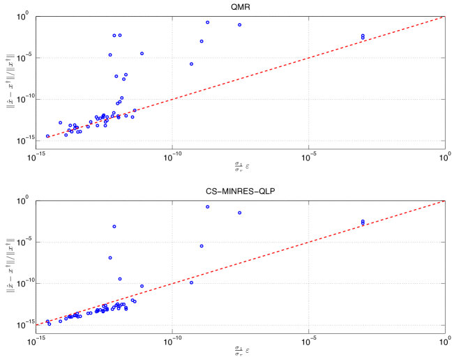
Fig. 2: 50 consistent singular complex symmetric systems. This figure is reproducible by C13Fig7_1.m.

Our second test set involves complex symmetric matrices that have a more wide-spread eigenspectrum than those in the first test set. Let $A=V\Lambda V^{T}\!$ be an eigenvalue decomposition of symmetric $A$ with $|\lambda_{1}|\geq\cdots\geq|\lambda_{n}|$. For $i=1,\ldots,n$, we define $d_{i}\equiv(2u_{i}-1)|\lambda_{1}|$, where $u_{i}\sim i.i.d.\ U(0,1)$ if $\lambda_{i}\neq 0$, or $d_{i}\equiv 0$ otherwise. Then the complex symmetric matrix $M\equiv VDV^{T}\!+iA$ has the same (numerical) rank as $A$, and its eigenspectrum is bounded by a ball of radius approximately equal to $|\lambda_{1}|$ on the complex plane. In Figure 3 we summarize the results of solving 50 such complex symmetric linear systems. CS-MINRES-QLP clearly behaved as stably as it did with the first test set. However, QMR is obviously more sensitive to the nonlinear spectrum: two problems did not converge, and about ten additional problems converged to their corresponding ${x}^{\dagger}$ with no more than four digits of accuracy.

Our third test set consists of linear LS problems (1), in which $A\equiv H$ in the upper plot of Figure 4 and $A\equiv M$ in the lower plot. In the case of $H$, CS-MINRES-QLP did not converge for two instances but agreed with the TSVD solutions to five or more digits for almost all other instances. In the case of $M$, CS-MINRES-QLP did not converge for five instances but agreed with the TSVD solutions to five or more digits for almost all other instances. Thus the algorithm is to some extent more sensitive to a nonlinear eigenspectrum in LS problems. This is also expected by the perturbation result that an upper bound of the relative error norm in a LS problem involves the square of $\kappa(A)$ [46, Theorem 5.2]. We did not run QMR on these test cases because the algorithm was not designed for LS problems.

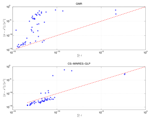
Fig. 3: 50 consistent singular complex symmetric systems. This figure is reproducible by C13Fig7_2.m.

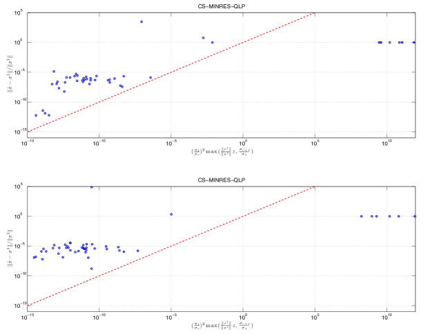
Fig. 4: 100 inconsistent singular complex symmetric systems. We used matrices $H$ in the upper plot and $M$ in the lower plot, where $H$ and $M$ are defined in Section 7.1. This figure is reproducible by C13Fig7_3.m.

7.2 Skew symmetric problems

Our fourth test collection consists of 50 skew symmetric linear systems and 50 singular skew symmetric LS problems (1). The matrices are constructed by $S=\mathtt{tril}(A)-\mathtt{tril}(A)^{T}\!$, where $\mathtt{tril}$ extracts the lower triangular part of a matrix. In both cases—linear systems in the upper subplot of Figure 5 and LS problems in the lower subplot—SS-MINRES-QLP did not converge for six instances but agreed with the TSVD solutions for more than ten digits of accuracy for almost all other instances.

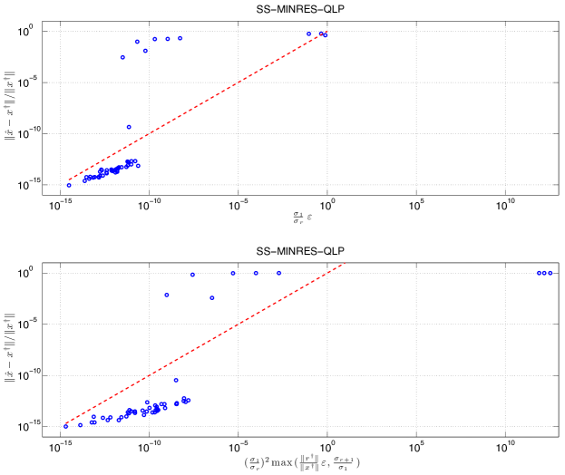
Fig. 5: 100 singular skew symmetric systems. Upper: 50 compatible linear systems. Lower: 50 LS problems. This figure is reproducible by C13Fig7_4.m.

7.3 Skew Hermitian problems

We also have created a test collection of 50 skew Hermitian linear systems and 50 skew Hermitian LS problems (1). Each skew Hermitian matrix is constructed as $T=S+iB$, where $S$ is skew symmetric as defined in the last test set, and $B\equiv A-\mathop{\operator@font diag}\nolimits([a_{11},\ldots,a_{nn}])$; in other words, $B$ is $A$ with the diagonal elements set to zero and is thus symmetric. We solve the problems using the original MINRES-QLP for Hermitian problems by the transformation $(iT)x\approx ib$. In the case of linear systems in the upper subplot of Figure 6, SH-MINRES-QLP did not converge for six instances. For the other instances SH-MINRES-QLP computed approximate solutions that matched the TSVD solutions for more than ten digits of accuracy. As for the LS problems in the lower subplot of Figure 6, only five instances did not converge.

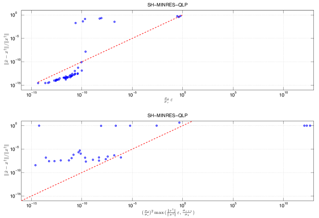
Fig. 6: 100 singular skew Hermitian systems. Upper: 50 compatible linear systems. Lower: 50 LS problems. This figure is reproducible by C13Fig7_5.m.

8 Conclusions

We take advantage of two Lanczos-like frameworks for square matrices or linear operators with special symmetries. In particular, the framework for complex-symmetric problems [2] is a special case of the Saunders-Simon-Yip process [43] with the starting vectors chosen to be $b$ and $\bar{b}$; we name the complex-symmetric process the Saunders process and the corresponding extended Krylov subspace from the $k$th iteration Saunders subspace $S_{k}(A,b)$.

CS-MINRES constructs its $k$th solution estimate from the short recursion $x_{k}=D_{k}t_{k}=x_{k-1}+\tau_{k}d_{k}$ (18), where $n$ separate triangular systems $R_{k}^{T}\!D_{k}^{T}\!=V_{k}^{*}$ are solved to obtain the $n$ elements of each direction $d_{1},\ldots,d_{k}$. (Only $d_{k}$ is obtained during iteration $k$, but it has $n$ elements.) In contrast, CS-MINRES-QLP constructs $x_{k}$ using orthogonal steps: $x_{k}=W_{k}u_{k}=x_{k-2}^{(2)}+w_{k-1}^{(3)}\mu_{k-1}^{(2)}+w_{k}^{(2)}\mu_{k}$; see (26)–(27). Only one triangular system $L_{k}u_{k}=t_{k}$ (23) is involved for each $k$. Thus CS-MINRES-QLP is numerically more stable than CS-MINRES. The additional work and storage are moderate, and efficiency is retained by transferring from CS-MINRES to CS-MINRES-QLP only when the estimated condition of $A$ exceeds an input parameter value.

TSVD is known to use rank-$k$ approximations to $A$ to find approximate solutions to $\min\|Ax-b\|$ that serve as a form of regularization. It is fair to conclude from the results that like other Krylov methods CS-MINRES have built-in regularization features [26, 25, 35]. Since CS-MINRES-QLP monitors more carefully and constructively the rank of $T_{k}$, which could be $k$ or $k\!-\!1$, we may say that regularization is a stronger feature in CS-MINRES-QLP, as we have shown in our numerical examples.

Like CS-MINRES and CS-MINRES-QLP, SS-MINRES and SS-MINRES-QLP are readily applicable to skew symmetric linear systems. Similarly, we have SH-MINRES and SH-MINRES-QLP for skew Hermitian problems. We summarize and compare these methods in Appendix C. CG and SYMMLQ for problems with these special symmetries can be derived likewise.

Software and reproducible research

Matlab 7.12 and Fortran 90/95 implementations of MINRES and MINRES-QLP for symmetric, Hermitian, skew symmetric, skew Hermitian, and complex symmetric linear systems with short-recurrence solution and norm estimates as well as efficient stopping conditions are available from the MINRES-QLP project website [10].

Following the philosophy of reliable reproducible computational research as advocated in [14, 8, 7], for each figure and example in this paper we mention either the source or the specific Matlab command. Our Matlab scripts are available at [10].

Acknowledgments

We thank our anonymous reviewers for their insightful suggestions for improving this manuscript. We are grateful for the feedback and encouragement from Peter Benner, Jed Brown, Xiao-Wen Chang, Youngsoo Choi, Heike Fassbender, Gregory Fasshauer, Ian Foster, Pedro Freitas, Roland Freund, Fred Hickernell, Ilse Ipsen, Sven Leyffer, Lek-Heng Lim, Lawrence Ma, Sayan Mukherjee, Todd Munson, Nilima Nigam, Christopher Paige, Xiaobai Sun, Paul Tupper, Stefan Wild, Jianlin Xia, and Yuan Yao during the development of this work. We appreciate the opportunities for presenting our algorithms in the 2012 Copper Mountain Conference on Iterative Methods, the 2012 Structured Numerical Linear and Multilinear Algebra Problems conference, and the 2013 SIAM Conference on Computational Science and Engineering. In particular, we thank Gail Pieper, Michael Saunders, and Daniel Szyld for their detailed comments, which resulted in a more polished exposition. We thank Heike Fassbender, Roland Freund, and Michael Saunders for helpful discussions on modified Krylov subspace methods during Lothar Reichel’s 60th birthday conference.

Appendix A Pseudocode of algorithms

1

input: $A,b,\sigma,\operatorname{maxit}$, where $A$ is complex symmetric, $\sigma$ is real or complex

2

3$v_{0}=0$,   $v_{1}=b$,   $\beta_{1}=\left\|b\right\|$,   $k=0$

4while $k\leq\operatorname{maxit}$ do

5       if $\beta_{k+1}>0$ then $v_{k+1}\leftarrow v_{k+1}/\beta_{k+1}$

6       else  STOP

7      

8      $k\leftarrow k+1$

9      $p_{k}=A\overline{v}_{k}-\sigma{\color[rgb]{0,0,0}\hbox{}\overline{v}_{k}}$

10      $\alpha_{k}=v_{k}^{*}p_{k}$

11      $p_{k}\leftarrow p_{k}-\alpha_{k}v_{k}$

12      $v_{k+1}=p_{k}-\beta_{k}v_{k-1}$

13      $\beta_{k+1}=\|v_{k+1}\|$

output: $V_{\ell},T_{\ell}$

Algorithm 1 Saunders process.

1

input: $A,b,\operatorname{maxit}$, where $A$ is skew symmetric

2

3$v_{0}=0$,   $v_{1}=b$,   $\beta_{0}=0$,   $\beta_{1}=\left\|b\right\|$,   $k=0$

4while $k\leq\operatorname{maxit}$ do

5       if $\beta_{k+1}>0$ then $v_{k+1}\leftarrow v_{k+1}/\beta_{k+1}$

6       else  STOP

7      

8      $k\leftarrow k+1$

9      $p_{k}=Av_{k}-v_{k}$

10      $v_{k+1}=p_{k}-\beta_{k}v_{k-1}$

11      $\beta_{k+1}=\|v_{k+1}\|$

output: $V_{\ell},T_{\ell}$

Algorithm 2 SS-Lanczos.

1

input: $A,b,\operatorname{maxit}$, where $A$ is skew Hermitian

2

3$v_{0}=0$,   $v_{1}={\color[rgb]{0,0,0}\hbox{}i}b$,   $\beta_{1}=\left\|b\right\|$,   $k=0$

4while $k\leq\operatorname{maxit}$ do

5       if $\beta_{k+1}>0$ then $v_{k+1}\leftarrow v_{k+1}/\beta_{k+1}$

6       else  STOP

7      

8      $k\leftarrow k+1$

9      $p_{k}=iAv_{k}-iv_{k}$

10      $\alpha_{k}=v_{k}^{*}p_{k}$

11      $p_{k}\leftarrow p_{k}-\alpha_{k}v_{k}$

12      $v_{k+1}=p_{k}-\beta_{k}v_{k-1}$

13      $\beta_{k+1}=\|v_{k+1}\|$

output: $V_{\ell},T_{\ell}$

Algorithm 3 SH-Lanczos.

1

input: $a,b$

2

3

4if $\left|b\right|=0$ then $c=1$,   $s=0$,   $r=a$

5 else if $\left|a\right|=0$ then

6      $c=0$,   $s=1$,   $r=b$

7else if $\left|b\right|\geq\left|a\right|$ then

8      $\tau=\left|a\right|/\left|b\right|$,   $c=1/\sqrt{1+\tau^{2}}$,   $s=c\tau(\overline{b/a})$,   $c\leftarrow c\tau$,   $r=b/\overline{s}$

9else if $\left|a\right|>\left|b\right|$ then

10      $\tau=\left|b\right|/\left|a\right|$,   $c=1/\sqrt{1+\tau^{2}}$,   $s=c(\overline{b/a})$,   $r=a/c$

11

output: $c,s,r$

Algorithm 4 Algorithm SymOrtho.

1

input: $A,b,\sigma,M$, where $A=A^{T}\in\mathbb{C}^{n\times n}$, $M=M^{T}\!\in\mathbb{C}^{n\times n}$ is nonsingular, $\sigma\in\mathbb{C}$

2

3

4$z_{0}=0$,   $z_{1}=b$,   Solve $Mq_{1}=z_{1}$,   $\beta_{1}=\sqrt{b^{T}\!q_{1}}$ [Initialize]

5

6$w_{0}=w_{-1}=0$,   $x_{-2}=x_{-1}=x_{0}=0$

7 $c_{0,1}\!=\!c_{0,2}\!=\!c_{0,3}\!=\!-1$,  $s_{0,1}\!=\!s_{0,2}\!=\!s_{0,3}\!=\!0$,  $\phi_{0}\!=\!\beta_{1}$,  $\tau_{0}\!=\!\omega_{0}\!=\!\chi_{-2}\!=\!\chi_{-1}\!=\!\chi_{0}\!=\!0$

8

9$\delta_{1}=\gamma_{-1}=\gamma_{0}=\eta_{-1}=\eta_{0}=\eta_{1}=\vartheta_{-1}=\vartheta_{0}=\vartheta_{1}=\mu_{-1}=\mu_{0}=0$,  $\mathcal{A}=0,\quad\kappa=1$

10

11$k=0$

12

13while no stopping condition is satisfied do

14       $k\leftarrow k+1$

15      

16      $p_{k}=Aq_{k}-\sigma q_{k}$,   $\alpha_{k}=\frac{1}{\beta_{k}^{2}}q_{k}^{T}\!p_{k}$ [Preconditioned Lanczos]

17      

18      $z_{k+1}=\frac{1}{\beta_{k}}p_{k}-\frac{\alpha_{k}}{\beta_{k}}z_{k}-\frac{\beta_{k}}{\beta_{k-1}}z_{k-1}$

19      

20      Solve $Mq_{k+1}=z_{k+1}$,   $\beta_{k+1}=\sqrt{q_{k+1}^{T}\!z_{k+1}}$

21      

22      if $k=1$ then $\rho_{k}=\|[\alpha_{k}\ \;\beta_{k+1}]\|$

23       else $\rho_{k}=\|[\beta_{k}\ \;\alpha_{k}\ \;\beta_{k+1}]\|$

24      

25      

26      $\delta_{k}^{(2)}=c_{k-1,1}\delta_{k}+s_{k-1,1}\alpha_{k}$ [Previous left reflection…]

27      

28      $\gamma_{k}=s_{k-1,1}\delta_{k}-c_{k-1,1}\alpha_{k}$ [on middle two entries of $\underline{T_{k}}e_{k}$…]

29      

30      ${\epsilon}_{k+1}=s_{k-1,1}\beta_{k+1}$ [produces first two entries in $\underline{T_{k+1}}e_{k+1}$]

31      

32      $\delta_{k+1}=-c_{k-1,1}\beta_{k+1}$

33      

34      $c_{k1},s_{k1},\gamma_{k}^{(2)}\leftarrow\text{SymOrtho}(\gamma_{k},\beta_{k+1})$ [Current left reflection]

35      

36      $c_{k2},s_{k2},\gamma_{k-2}^{(6)}\leftarrow\text{SymOrtho}(\gamma_{k-2}^{(5)},\epsilon_{k})$ [First right reflection]

37      

38      $\delta_{k}^{(3)}=s_{k2}\vartheta_{k-1}-c_{k2}\delta_{k}^{(2)}$,   $\gamma_{k}^{(3)}=-c_{k2}\gamma_{k}^{(2)}$,   $\eta_{k}=s_{k2}\gamma_{k}^{(2)}$

39      

40      $\vartheta_{k-1}^{(2)}=c_{k2}\vartheta_{k-1}+s_{k2}\delta_{k}^{(2)}$

41      

42      $c_{k3},s_{k3},\gamma_{k-1}^{(5)}\leftarrow\text{SymOrtho}(\gamma_{k-1}^{(4)},\delta_{k}^{(3)})$ [Second right reflection…]

43      

44      $\vartheta_{k}=s_{k3}\gamma_{k}^{(3)}$,   $\gamma_{k}^{(4)}=-c_{k3}\gamma_{k}^{(3)}$ [to zero out $\delta_{k}^{(3)}$]

45      

46      $\tau_{k}^{(2)}=c_{k1}\tau_{k}$ [Last element of $t_{k}$]

47      

48      $\phi_{k}=\phi_{k-1}|s_{k1}|$,  $\psi_{k-1}=\phi_{k-1}\|[\smash{\gamma_{k}\ \;\delta_{k+1}}]\|$ [Update $\|r_{k}\|$, $\|Ar_{k-1}\|$]

49      

50      if $k=1$ then $\gamma_{\min}=\gamma_{1}$

51       else $\gamma_{\min}\leftarrow\min{\{\gamma_{\min},\gamma_{k-2}^{(6)},\gamma_{k-1}^{(5)},|\gamma_{k}^{(4)}|\}}$

52      

53      

54      $\mathcal{A}^{(k)}=\max{\{\mathcal{A}^{(k-1)},\rho_{k},\gamma_{k-2}^{(6)},\gamma_{k-1}^{(5)},|\gamma_{k}^{(4)}|\}}$ [Update $\|A\|$]

55      

56      $\omega_{k}=\|[\smash{\omega_{k-1}\ \;\tau_{k}^{(2)}}]\|$,   $\kappa\leftarrow\mathcal{A}^{(k)}/\gamma_{\min}$ [Update $\|Ax_{k}\|$, $\kappa(A)$]

57      

58      $w_{k}=-(c_{k2}/\beta_{k})q_{k}+s_{k2}w_{k-2}^{(3)}$ [Update $w_{k-2}$, $w_{k-1}$, $w_{k}$]

59      

60      $w_{k-2}^{(4)}=(s_{k2}/\beta_{k})q_{k}+c_{k2}w_{k-2}^{(3)}$

61      if $k>2$ then $w_{k}^{(2)}=s_{k3}w_{k-1}^{(2)}-c_{k3}w_{k}$,   $w_{k-1}^{(3)}=c_{k3}w_{k-1}^{(2)}+s_{k3}w_{k}$

62      

63      

64      if $k>2$ then $\mu_{k-2}^{(3)}=(\tau_{k-2}^{(2)}-\eta_{k-2}\mu_{k-4}^{(4)}-\vartheta_{k-2}\mu_{k-3}^{(3)})/\gamma_{k-2}^{(6)}$

65       [Update $\mu_{k-2}$]

66      

67      if $k>1$ then $\mu_{k-1}^{(2)}=(\tau_{k-1}^{(2)}-\eta_{k-1}\mu_{k-3}^{(3)}-\vartheta_{k-1}^{(2)}\mu_{k-2}^{(3)})/\gamma_{k-1}^{(5)}$

68       [Update $\mu_{k-1}$]

69      

70      if $\gamma_{k}^{(4)}\neq 0$ then $\mu_{k}=(\tau_{k}^{(2)}-\eta_{k}\mu_{k-2}^{(3)}-\vartheta_{k}\mu_{k-1}^{(2)})/\gamma_{k}^{(4)}$

71       else $\mu_{k}=0$

72       [Compute $\mu_{k}$]

73      

74      $x_{k-2}^{(2)}=x_{k-3}^{(2)}+\mu_{k-2}^{(3)}w_{k-2}^{(3)}$ [Update $x_{k-2}$]

75      

76      $x_{k}=x_{k-2}^{(2)}+\mu_{k-1}^{(2)}w_{k-1}^{(3)}+\mu_{k}w_{k}^{(2)}$ [Compute $x_{k}$]

77      

78      $\chi_{k-2}^{(2)}=\|[\smash{\chi_{k-3}^{(2)}\ \;\mu_{k-2}^{(3)}}]\|$ [Update $\|x_{k-2}\|$]

79      

80      $\chi_{k}=\|[\smash{\chi_{k-2}^{(2)}\ \;\mu_{k-1}^{(2)}\ \;\mu_{k}}]\|$ [Compute $\|x_{k}\|$]

81      

82

83$x=x_{k}$,  $\phi=\phi_{k}$,  $\psi=\phi_{k}\|[\smash{\gamma_{k+1}\ \;\delta_{k+2}}]\|$,  $\chi=\chi_{k}$,  $\mathcal{A}=\mathcal{A}^{(k)}$,  $\omega=\omega_{k}$

84

output: $x,\phi,\psi,\chi,\mathcal{A},\kappa,\omega$

85

86

87 [$c,s\leftarrow\text{SymOrtho}(a,b)$ is a stable form for computing $r=\sqrt{a^{2}+b^{2}}$, $c=\frac{a}{r}$, $s=\frac{b}{r}$]

88

Algorithm 5 Preconditioned CS-MINRES-QLP to solve $(A-\sigma I)x\approx b$.

Appendix B Stopping conditions and norm estimates

This section derives several short-recurrence norm estimates in MINRES and MINRES-QLP for complex symmetric and skew Hermitian systems. As before, we assume exact arithmetic throughout, so that $V_{k}$ and $Q_{k}$ are orthonormal. Table 1 summarizes how these norm estimates are used to formulate six groups of concerted stopping conditions. The second NRBE test is specifically designed for LS problems, which have the properties $r\neq 0$ but $A^{*}r=0$; it is inspired by Stewart [48] and stops the algorithm when $\|A^{*}r_{k}\|$ is small relative to its upper bound $\|A\|\|r_{k}\|$.

Table 1: Stopping conditions in CS-MINRES and SH-MINRES. NRBE means normwise relative backward error, and $\mathit{tol}$, $\mathit{maxit}$, $\mathit{maxcond}$ and $\mathit{maxxnorm}$ are input parameters. All norms and $\kappa(A)$ are estimated by CS-MINRES and SH-MINRES.

Lanczos	NRBE	Regularization attempts
$\beta_{k+1}\leq n\|A\|\varepsilon$	$\|r_{k}\|/\left(\|A\|\|x_{k}\|+\|b\|\right)\leq\max(\mathit{tol},\varepsilon)$	$\kappa(A)\geq\max(\mathit{maxcond},\frac{1}{\varepsilon})$
$k=\mathit{maxit}$	$\|\overline{A}r_{k}\|/\left(\|A\|\|r_{k}\|\right)\leq\max(\mathit{tol},\varepsilon)$	$\|x_{k}\|\geq\mathit{maxxnorm}$
CS-MINRES	Degenerate cases	Erroneous input
$\left|\gamma_{k}^{(4)}\right|<\varepsilon$	$\beta_{1}=0\quad\Rightarrow\quad x^{\dagger}=0$	$y^{*}(Az)\neq\pm z^{*}(\overline{A}y)$
	$\beta_{2}=0\quad\Rightarrow\quad x^{\dagger}=\overline{b}/\alpha_{1}$	$\qquad\Rightarrow\qquad A\neq\pm A^{T}\!$

B.1 Residual and residual norm

First we derive recurrence relations for $r_{k}$ and its norm $\|r_{k}\|=|\phi_{k}|$. The results are true for CS-MINRES and CS-MINRES-QLP.

Lemma 5.

Without loss of generality, let $x_{0}=0$. We have the results below.

1. $r_{0}=b$ and $\|r_{0}\|=\phi_{0}=\beta_{1}$.

2. For $k=1,\ldots,\ell-1$, $\|r_{k}\|=|\phi_{k}|=|\phi_{k-1}||s_{k}|\geq|\phi_{k-1}|>0$. Thus $\|r_{k}\|$ is monotonically decreasing.

3. At the last iteration $\ell$,

   1. If $\mathop{\operator@font rank}\nolimits(L_{\ell})=\ell$, then $\|r_{\ell}\|=\phi_{\ell}=0$.

   2. If $\mathop{\operator@font rank}\nolimits(L_{\ell})=\ell\!-\!1$, then $\|r_{\ell}\|=|\phi_{\ell-1}|>0$.

Proof.

1. Obvious.

2. If $k<\ell$, from (9)–(18) with $R_{k}y_{k}=t_{k}$ we have

   $$r_{k} =V_{k+1}Q_{k}^{*}{\begin{pmatrix}{\begin{bmatrix}t_{k}\\ \phi_{k}\end{bmatrix}}-{\begin{bmatrix}R_{k}\\ 0\end{bmatrix}}y_{k}\end{pmatrix}}=\phi_{k}V_{k+1}Q_{k}^{*}e_{k+1}.$$ (34)

   We have $\|r_{k}\|=|\phi_{k}|=|\phi_{k-1}||s_{k}|>0$; see (12)–(14).

3. If $T_{\ell}$ is nonsingular, $r_{\ell}=0$. Otherwise $Q_{\ell-1,\ell}$ has made the last row of $R_{\ell}$ zero, so the last row and column of $L_{\ell}$ are zero; see (29). Thus $r_{\ell}=r_{\ell-1}\neq 0$.

∎

B.2 Norm of $A^{*}r_{k}$

For incompatible systems, $r_{k}$ will never be zero. However, all LS solutions satisfy $A^{*}Ax=A^{*}b$, so that $A^{*}r=0$. We therefore need a stopping condition based on the size of $\|A^{*}r_{k}\|=\psi_{k}$. We present efficient recurrence relations for $\|A^{*}r_{k}\|$ in the following lemma. We also show that $A^{*}r_{k}$ is orthogonal to $\mathcal{K}_{k}(A,\overline{b})$.

Lemma 6 ($A^{*}r_{k}$ and $\psi_{k}\equiv\|A^{*}r_{k}\|$ for CS-MINRES).

1. If $k<\ell$, then $\mathop{\operator@font rank}\nolimits(L_{k})=k$, $\overline{A}r_{k}=\|r_{k}\|(\overline{\gamma}_{k+1}\overline{v}_{k+1}+\delta_{k+2}\overline{v}_{k+2})$ and $\psi_{k}=\|r_{k}\|\|[\gamma_{k+1}\ \;\delta_{k+2}]\|$, where $\delta_{k+2}=0$ if $k=\ell\!-\!1$.

2. At the last iteration $\ell$,

   1. If $\mathop{\operator@font rank}\nolimits(L_{\ell})=\ell$, then $Ar_{\ell}=0$ and $\psi_{\ell}=0$.

   2. If $\mathop{\operator@font rank}\nolimits(L_{\ell})=\ell\!-\!1$, then $Ar_{\ell}=Ar_{\ell-1}=0$, and $\psi_{\ell}=\psi_{\ell-1}=0$.

Proof.

Case 2 follows directly from Lemma 5. We prove the first case here. For $k<\ell$, $R_{k}$ is nonsingular. From (9)–(18) with $R_{k}y_{k}=t_{k}$ we have

$$\overline{A}r_{k} =\phi_{k}\overline{V}\!_{k+2}\underline{\overline{T}\!_{k+1}}Q_{k}^{*}e_{k+1},\text{ by }(\ref{rk7})$$

$$Q_{k}\underline{T_{k+1}}^{T}\! =Q_{k}{\begin{bmatrix}T_{k+1}&\beta_{k+2}e_{k+1}\end{bmatrix}}=Q_{k}{\begin{bmatrix}T_{k}&\beta_{k+1}e_{k}&0\\ \beta_{k+1}e_{k}^{T}&\alpha_{k+1}&\beta_{k+2}\end{bmatrix}},$$

$$e_{k+1}^{T}Q_{k}\underline{T_{k+1}}^{T}\! ={\begin{bmatrix}0&\gamma_{k+1}&\delta_{k+2}\end{bmatrix}},$$

by (13). We take $\delta_{k+2}=0$ if $k=\ell-1$, so

$$\overline{A}r_{k} =\tau_{k+1}\overline{V}\!_{k+2}{\begin{bmatrix}0&\gamma_{k+1}&\delta_{k+2}\end{bmatrix}}^{*}=\tau_{k+1}\left(\overline{\gamma}_{k+1}\overline{v}_{k+1}+\delta_{k+2}\overline{v}_{k+2}\right),$$

$$\psi_{k}^{2} \equiv\|\overline{A}r_{k}\|^{2}=\|r_{k}\|^{2}\left([\gamma_{k+1}]^{2}+[\delta_{k+2}]^{2}\right).$$

The result follows. ∎

Typically $\|\overline{A}r_{k}\|$ is not monotonic, while clearly $\|r_{k}\|$ is monotonically decreasing. In the singular system $A=U\Sigma U^{T}\!$, let $U={\begin{bmatrix}U_{1}\!&\!U_{2}\end{bmatrix}}$, where the singular vectors $U_{1}$ correspond to nonzero singular values. Then $P_{A}\equiv U_{1}U_{1}^{*}$ and $P^{\perp}_{A}\equiv U_{2}U_{2}^{*}$ are orthogonal projectors [52] onto the range and nullspace of $A$. For general linear LS problems, Chang et al. [5] characterize the dynamics of $\|r_{k}\|$ and $\|A^{*}r_{k}\|$ in three phases defined in terms of the ratios among $\|r_{k}\|$, $\|P_{A}r_{k}\|$, and $\|P^{\perp}_{A}r_{k}\|$, and propose two new stopping criteria for iterative solvers. The expositions in [1, 34] show that these estimates are cheaply computable in CGLS and LSQR [39, 40]. These results are likely applicable to CS-MINRES.

B.3 Matrix norms

From the Lanczos process, $\|A\|\geq\|V_{k+1}^{*}A\overline{V}\!_{k}\|=\|\underline{T_{k}}\|$. Define

$$\mathcal{A}^{(0)}\equiv 0,\quad\mathcal{A}^{(k)}\equiv\max_{j=1,\ldots,k}\left\{\|\underline{T_{j}}e_{j}\|\right\}=\max\left\{\mathcal{A}^{(k-1)},\|\underline{T_{k}}e_{k}\|\right\}\text{ for }k\geq 1.$$ (35)

Then $\|A\|\geq\|\underline{T_{k}}\|\geq\mathcal{A}^{(k)}$. Clearly, $\mathcal{A}^{(k)}$ is monotonically increasing and is thus an improving estimate for $\|A\|$ as $k$ increases. By the property of QLP decomposition in (8) and (4.1), we could easily extend (35) to include the largest diagonal of $L_{k}$:

$$\mathcal{A}^{(0)}\equiv 0,\quad\mathcal{A}^{(k)}\equiv\max\{\mathcal{A}^{(k-1)},\,\|\underline{T_{k}}e_{k}\|,\,\gamma_{k-2}^{(6)},\,\gamma_{k-1}^{(5)},\,|\gamma_{k}^{(4)}|\}\text{ for }k\geq 1,$$ (36)

which uses quantities readily available from CS-MINRES and gives satisfactory, if not extremely accurate, estimates for the order of $\|A\|$.

B.4 Matrix condition numbers

We again apply the property of the QLP decomposition in (8) and (4.1) to estimate $\kappa(\underline{T_{k}})$, which is a lower bound for $\kappa(A)$:

$$\gamma_{\min} \leftarrow\min\{\gamma_{1},\gamma_{2}^{(2)}\},\quad\gamma_{\min}\leftarrow\min\{\gamma_{\min},\gamma_{k-2}^{(6)},\,\gamma_{k-1}^{(5)},\,|\gamma_{k}^{(4)}|\}\text{ for }k\geq 3,$$

$$\kappa^{(0)} \equiv 1,\quad\kappa^{(k)}\equiv\max\left\{\kappa^{(k-1)},\frac{\mathcal{A}^{(k)}}{\gamma_{\min}}\right\}\text{ for }k\geq 1.$$ (37)

B.5 Solution norms

For CS-MINRES-QLP, we derive a recurrence relation for $\|x_{k}\|$ whose cost is as low as computing the norm of a $3$- or $4$-vector. This recurrence relation is not applicable to CS-MINRES standalone.

Since $\|x_{k}\|=\|\overline{V}\!_{k}P_{k}u_{k}\|=\|u_{k}\|$, we can estimate $\|x_{k}\|$ by computing $\chi_{k}\equiv\|u_{k}\|$. However, the last two elements of $u_{k}$ change in $u_{k+1}$ (and a new element $\mu_{k+1}$ is added). We therefore maintain $\chi_{k-2}$ by updating it and then using it according to

$$\chi_{k-2}^{(2)}=\|[\chi_{k-3}^{(2)}\ \;\mu_{k-2}^{(3)}]\|,\quad\chi_{k}=\|[\chi_{k-2}^{(2)}\ \;\mu_{k-1}^{(2)}\ \;\mu_{k}]\|{\color[rgb]{0,0,0}\hbox{};}$$

cf. (26) and (27). Thus $\chi_{k-2}^{(2)}$ increases monotonically but we cannot guarantee that $\|x_{k}\|$ and its recurred estimate $\chi_{k}$ are increasing, and indeed they are not in some examples. But the trend for $\chi_{k}$ is generally increasing, and $\chi_{k}^{(2)}$ is theoretically a better estimate than $\chi_{k}$ for $\|x_{k}\|$. In LS problems, when $\gamma_{k}^{(4)}$ is small enough in magnitude, it also means $\|x_{k}\|=\|y_{k}\|=\|u_{k}\|$ is large—and when this quantity is larger than $\mathit{maxxnorm}$, it usually means that we should do only a partial update of $x_{k}=x_{k-2}^{(2)}+w_{k-1}^{(3)}\mu_{k-1}^{(2)}$. If it still exceeds $\mathit{maxxnorm}$ in length, then we do no update, namely, $x_{k}=x_{k-2}^{(2)}$.

B.6 Projection norms

In applications requiring nullvectors [6], $Ax_{k}$ is useful. Other times, the projection of the right-hand side $b$ onto $\mathcal{K}_{k}(A,\overline{b})$ is required [42]. For the recurrence relations of $Ax_{k}$ and its norm, we have

$$Ax_{k} =A\overline{V}\!_{k}y_{k}=V_{k+1}\underline{T_{k}}y_{k}=V_{k+1}Q_{k}^{*}{\begin{bmatrix}R_{k}\\ 0\end{bmatrix}}y_{k}=V_{k+1}Q_{k}^{*}{\begin{bmatrix}t_{k}\\ 0\end{bmatrix}},$$

$$\omega_{k}^{2} \equiv\|Ax_{k}\|^{2}=\|t_{k}\|^{2}=\|t_{k-1}\|^{2}+(\tau_{k}^{(2)})^{2}=\omega_{k-1}^{2}+(\tau_{k}^{(2)})^{2}=\|{\left[\begin{smallmatrix}\omega_{k-1}&\tau_{k}^{(2)}\end{smallmatrix}\right]}\|^{2}.$$

Thus $\{\omega_{k}\}$ is monotonic.

Appendix C Comparison of Lanczos-based solvers

We compare our new solvers with CG, SYMMLQ, MINRES, and MINRES-QLP in Tables 3–3 in terms of subproblem definitions, basis, solution estimates, flops, and memory. A careful implementation of SYMMLQ computes $x_{k}$ in $\mathop{\mathrm{range}}(V_{k+1})$; see [6, Section 2.2.2] for a proof. All solvers need storage for $v_{k}$, $v_{k+1}$, $x_{k}$, and a product $p_{k}=Av_{k}$ or $A\overline{v}_{k}$ each iteration. Some additional work-vectors are needed for each method (e.g., $d_{k-1}$ and $d_{k}$ for MINRES or CS-MINRES, giving 7 work-vectors in total). We note that even for Hermitian and skew Hermitian problems $Ax=b$, the subproblems of CG, SYMMLQ, MINRES, and MINRES-QLP are real.

Table 2: Subproblems defining $x_{k}$ for CG, SYMMLQ, MINRES, MINRES-QLP, CS-MINRES, CS-MINRES-QLP, SS-MINRES, SH-MINRES-QLP, SH-MINRES, and SH-MINRES-QLP.

Method	Subproblem	Factorization	Estimate of $x_{k}$
cgLanczos	$T_{k}y_{k}=\beta_{1}e_{1}$	Cholesky:	$x_{k}=V_{k}y_{k}$
[27, 38, 44]		$T_{k}=L_{k}D_{k}L_{k}^{T}\!$	$\quad\in{\color[rgb]{0,0,0}\hbox{}\mathcal{K}_{k}(A,b)}$
SYMMLQ	$y_{k+1}=\arg\min_{y\in\mathbb{R}^{k+1}}\|y\|$	LQ:	$x_{k}=V_{k+1}y_{k+1}$
[38, 6]	s.t. $\underline{T_{k}^{T}\!}y=\beta_{1}e_{1}$	$\underline{T_{k}}^{T}\!Q_{k}^{T}\!={\begin{bmatrix}L_{k}&\!\!\!0\end{bmatrix}}$	$\in{\color[rgb]{0,0,0}\hbox{}\mathcal{K}_{k+1}(A,b)}$
MINRES [38],[6]-[11]	${\displaystyle y_{k}=\arg\min_{y\in\mathbb{R}^{k}}\|\underline{T_{k}}y-\beta_{1}e_{1}\|}$	QR:	$x_{k}=V_{k}y_{k}$
SS-MINRES		$Q_{k}\underline{T_{k}}=\raisebox{4.0pt}{${\begin{bmatrix}R_{k}\\ 0\end{bmatrix}}$}$	$\quad\in{\color[rgb]{0,0,0}\hbox{}\mathcal{K}_{k}(A,b)}$
MINRES-QLP ​​ [6]-[11]	$y_{k}=\arg\min_{y\in\mathbb{R}^{k}}\|y\|$	QLP:	$x_{k}=V_{k}y_{k}$
SS-MINRES-QLP	s.t. $y\in\arg\min\|\underline{T_{k}}y-\beta_{1}e_{1}\|$​​	$Q_{k}\underline{T_{k}}P_{k}=\raisebox{4.0pt}{${\begin{bmatrix}L_{k}\\ 0\end{bmatrix}}$}$	$\quad\in{\color[rgb]{0,0,0}\hbox{}\mathcal{K}_{k}(A,b)}$
SH-MINRES	${\displaystyle y_{k}=\arg\min_{y\in\mathbb{R}^{k}}\|\underline{T_{k}}y-\beta_{1}e_{1}\|}$	QR:	$x_{k}={\color[rgb]{0,0,0}\hbox{}V}\!_{k}y_{k}$
		$Q_{k}\underline{T_{k}}=\raisebox{4.0pt}{${\begin{bmatrix}R_{k}\\ 0\end{bmatrix}}$}$	$\quad\in{\color[rgb]{0,0,0}\hbox{}\mathcal{K}_{k}(iA,ib)}$
SH-MINRES-QLP ​​	$y_{k}=\arg\min_{y\in\mathbb{R}^{k}}\|y\|$	QLP:	$x_{k}={\color[rgb]{0,0,0}\hbox{}V}\!_{k}y_{k}$
	s.t. $y\in\arg\min\|\underline{T_{k}}y-\beta_{1}e_{1}\|$​​	$Q_{k}\underline{T_{k}}P_{k}=\raisebox{4.0pt}{${\begin{bmatrix}L_{k}\\ 0\end{bmatrix}}$}$	$\quad\in{\color[rgb]{0,0,0}\hbox{}\mathcal{K}_{k}(iA,ib)}$
CS-MINRES	${\displaystyle y_{k}=\arg\min_{y\in\mathbb{C}^{k}}\|\underline{T_{k}}y-\beta_{1}e_{1}\|}$	QR:	$x_{k}=\overline{V}\!_{k}y_{k}$
		$Q_{k}\underline{T_{k}}=\raisebox{4.0pt}{${\begin{bmatrix}R_{k}\\ 0\end{bmatrix}}$}$	$\quad\in{\color[rgb]{0,0,0}\hbox{}\mathcal{S}_{k}(A,b)}$
CS-MINRES-QLP ​​	$y_{k}=\arg\min_{y\in\mathbb{C}^{k}}\|y\|$	QLP:	$x_{k}=\overline{V}\!_{k}y_{k}$
	s.t. $y\in\arg\min\|\underline{T_{k}}y-\beta_{1}e_{1}\|$​​	$Q_{k}\underline{T_{k}}P_{k}=\raisebox{4.0pt}{${\begin{bmatrix}L_{k}\\ 0\end{bmatrix}}$}$	$\quad\in{\color[rgb]{0,0,0}\hbox{}\mathcal{S}_{k}(A,b)}$

Table 3: Bases, subproblem solutions, storage, and work for each method.

Method	New Basis	$\quad\quad\quad z_{k},t_{k},u_{k}$	$x_{k}$ Estimate	​​vecs  flops​​
cgLanczos	$W_{k}\equiv V_{k}L_{k}^{-T}$	$L_{k}D_{k}z_{k}=\beta_{1}e_{1}$	$x_{k}\!=\!W_{k}z_{k}$	5   $\ 8n$
SYMMLQ	$W_{k}\equiv V_{k+1}Q_{k}^{T}{\begin{bmatrix}I_{k}\\ 0\end{bmatrix}}$​​	$L_{k}z_{k}\!=\!\beta_{1}e_{1}$	$x_{k}\!=\!W_{k}z_{k}$	6   $\ 9n$
MINRES	$D_{k}\equiv V_{k}R_{k}^{-1}$	$\ \ \ \ t_{k}\!=\!\beta_{1}\rule[-8.1805pt]{0.0pt}{22.81938pt}{\begin{bmatrix}I_{k}&\!\!\!0\end{bmatrix}}Q_{k}e_{1}$​​	$x_{k}\!=\!D_{k}t_{k}$	7   $\ 9n$
SS-MINRES
SH-MINRES
MINRES-QLP ​​	$W_{k}\equiv V_{k}P_{k}$	$L_{k}u_{k}\!=\!\beta_{1}\rule[-8.1805pt]{0.0pt}{22.81938pt}{\begin{bmatrix}I_{k}&\!\!\!0\end{bmatrix}}Q_{k}e_{1}$​​	$x_{k}\!=\!W_{k}u_{k}$	8   $14n$
SS-MINRES-QLP
SH-MINRES-QLP
CS-MINRES	$D_{k}\equiv\overline{V}\!_{k}R_{k}^{-1}$	$\ \ \ \ t_{k}\!=\!\beta_{1}\rule[-8.1805pt]{0.0pt}{22.81938pt}{\begin{bmatrix}I_{k}&\!\!\!0\end{bmatrix}}Q_{k}e_{1}$​​	$x_{k}\!=\!D_{k}t_{k}$	7   $\ 9n$
CS-MINRES-QLP ​​	$W_{k}\equiv\overline{V}\!_{k}P_{k}$	$L_{k}u_{k}\!=\!\beta_{1}\rule[-8.1805pt]{0.0pt}{22.81938pt}{\begin{bmatrix}I_{k}&\!\!\!0\end{bmatrix}}Q_{k}e_{1}$​​	$x_{k}\!=\!W_{k}u_{k}$	8   $14n$

The submitted manuscript has been created by the University of Chicago as Operator of Argonne National Laboratory (“Argonne”) under Contract DE-AC02-06CH11357 with the U.S. Department of Energy. The U.S. Government retains for itself, and others acting on its behalf, a paid-up, nonexclusive, irrevocable worldwide license in said article to reproduce, prepare derivative works, distribute copies to the public, and perform publicly and display publicly, by or on behalf of the Government.

References

• [1] M. Arioli and S. Gratton. Least-squares problems, normal equations, and stopping criteria for the conjugate gradient method. Technical Report RAL-TR-2008-008, Rutherford Appleton Laboratory, Oxfordshire, UK, 2008.
• [2] A. Bunse-Gerstner and R. Stöver. On a conjugate gradient-type method for solving complex symmetric linear systems. Linear Algebra and its Applications, 287(1):105–123, 1999.
• [3] R. H. Chan and X.-Q. Jin. Circulant and skew-circulant preconditioners for skew-Hermitian type Toeplitz systems. BIT, 31(4):632–646, 1991.
• [4] R. H.-F. Chan and X.-Q. Jin. An Introduction to Iterative Toeplitz Solvers. Society for Industrial and Applied Mathematics, 2007.
• [5] X.-W. Chang, C. C. Paige, and D. Titley-Péloquin. Stopping criteria for the iterative solution of linear least squares problems. SIAM J. Matrix Anal. Appl., 31(2):831–852, 2009.
• [6] S.-C. T. Choi. Iterative Methods for Singular Linear Equations and Least-Squares Problems. PhD thesis, ICME, Stanford University, 2006.
• [7] S.-C. T. Choi. MINRES-QLP pack and reliable reproducible research via staunch scientific software. In First Workshop on Sustainable Software for Science: Practice and Experiences, Denver, Colorado, 2013.
• [8] S.-C. T. Choi, D. L. Donoho, A. G. Flesia, X. Huo, O. Levi, and D. Shi. About Beamlab—a toolbox for new multiscale methodologies. http://www-stat.stanford.edu/~beamlab/, 2002.
• [9] S.-C. T. Choi, C. C. Paige, and M. A. Saunders. MINRES-QLP: A Krylov subspace method for indefinite or singular symmetric systems. SIAM J. Sci. Comput., 33(4):1810–1836, 2011.
• [10] S.-C. T. Choi and M. A. Saunders. MINRES-QLP MATLAB package. http://code.google.com/p/minres-qlp/, 2011.
• [11] S.-C. T. Choi and M. A. Saunders. ALGORITHM & DOCUMENTATION: MINRES-QLP for singular symmetric and Hermitian linear equations and least-squares problems. Technical Report ANL/MCS-P3027-0812, Computation Institute, University of Chicago, IL, 2012.
• [12] S.-C. T. Choi and M. A. Saunders. MINRES-QLP FORTRAN 90 package. http://code.google.com/p/minres-qlp/, 2012.
• [13] S.-C. T. Choi and M. A. Saunders. ALGORITHM xxx: MINRES-QLP for singular symmetric and Hermitian linear equations and least-squares problems. ACM Trans. Math. Software, 2014.
• [14] J. Claerbout. Hypertext documents about reproducible research. http://sepwww.stanford.edu/doku.php?id=sep:research:reproducible.
• [15] I. S. Duff. MA57—a code for the solution of sparse symmetric definite and indefinite systems. ACM Trans. Math. Software, 30(2):118–144, 2004.
• [16] R. Fletcher. Conjugate gradient methods for indefinite systems. In Numerical Analysis (Proc 6th Biennial Dundee Conf., Univ. Dundee, Dundee, 1975), pages 73–89. Lecture Notes in Math., Vol. 506. Springer, Berlin, 1976.
• [17] L. Foster. SJsingular—MATLAB toolbox for managing the SJSU singular matrix collection. http://www.math.sjsu.edu/singular/matrices/SJsingular.html, 2008.
• [18] L. Foster. San Jose State University singular matrix database. http://www.math.sjsu.edu/singular/matrices/, 2009.
• [19] R. W. Freund. Conjugate gradient-type methods for linear systems with complex symmetric coefficient matrices. SIAM J. Sci. Statist. Comput., 13(1):425–448, 1992.
• [20] R. W. Freund and N. M. Nachtigal. QMR: a quasi-minimal residual method for non-Hermitian linear systems. Numer. Math., 60(3):315–339, 1991.
• [21] D. F. Gleich and L.-H. Lim. Rank aggregation via nuclear norm minimization. In Proceedings of the 17th ACM SIGKDD International Conference on Knowledge Discovery and Data Mining, KDD ’11, pages 60–68, New York, NY, USA, 2011. ACM.
• [22] G. H. Golub and C. F. Van Loan. Matrix computations. Johns Hopkins University Press, 4th edition, 2012.
• [23] C. Greif and J. Varah. Iterative solution of skew-symmetric linear systems. SIAM J. Matrix Anal. Appl., 31(2):584–601, 2009.
• [24] J. Hadamard. Sur les problèmes aux dérivées partielles et leur signification physique. Princeton University Bulletin, XIII(4):49–52, 1902.
• [25] M. Hanke and J. G. Nagy. Restoration of atmospherically blurred images by symmetric indefinite conjugate gradient techniques. Inverse Problems, 12(2):157–173, 1996.
• [26] P. C. Hansen and D. P. O’Leary. The use of the L-curve in the regularization of discrete ill-posed problems. SIAM J. Sci. Comput., 14(6):1487–1503, 1993.
• [27] M. R. Hestenes and E. Stiefel. Methods of conjugate gradients for solving linear systems. J. Research Nat. Bur. Standards, 49:409–436, 1952.
• [28] N. J. Higham. Functions of matrices. Society for Industrial and Applied Mathematics, Philadelphia, PA, 2008. Theory and computation.
• [29] R. A. Horn and C. R. Johnson. Matrix analysis. Cambridge University Press, Cambridge, 1990. Corrected reprint of the 1985 original.
• [30] R. A. Horn and C. R. Johnson. Topics in matrix analysis. Cambridge University Press, Cambridge, 1991.
• [31] D. A. Huckaby and T. F. Chan. On the convergence of Stewart’s QLP algorithm for approximating the SVD. Numer. Algorithms, 32(2-4):287–316, 2003.
• [32] F. Incertis. A skew-symmetric formulation of the algebraic riccati equation problem. Automatic Control, IEEE Transactions on, 29(5):467–470, 1984.
• [33] X. Jiang, L.-H. Lim, Y. Yao, and Y. Ye. Statistical ranking and combinatorial Hodge theory. Math. Program., 127(1, Ser. B):203–244, 2011.
• [34] P. Jiránek and D. Titley-Péloquin. Estimating the backward error in LSQR. SIAM J. Matrix Anal. Appl., 31(4):2055–2074, 2010.
• [35] M. Kilmer and G. W. Stewart. Iterative regularization and MINRES. SIAM J. Matrix Anal. Appl., 21(2):613–628, 1999.
• [36] C. Lanczos. Applied analysis. Englewood Cliffs, N.J., Prentice Hall, 1956.
• [37] C. C. Paige. Error analysis of the Lanczos algorithm for tridiagonalizing a symmetric matrix. J. Inst. Math. Appl., 18(3):341–349, 1976.
• [38] C. C. Paige and M. A. Saunders. Solution of sparse indefinite systems of linear equations. SIAM J. Numer. Anal., 12(4):617–629, 1975.
• [39] C. C. Paige and M. A. Saunders. LSQR: an algorithm for sparse linear equations and sparse least squares. ACM Trans. Math. Software, 8(1):43–71, 1982.
• [40] C. C. Paige and M. A. Saunders. zAlgorithm 583; LSQR: Sparse linear equations and least-squares problems. ACM Trans. Math. Software, 8(2):195–209, 1982.
• [41] Y. Saad and M. H. Schultz. GMRES: a generalized minimal residual algorithm for solving nonsymmetric linear systems. SIAM J. Sci. Statist. Comput., 7(3):856–869, 1986.
• [42] M. A. Saunders. Computing projections with LSQR. BIT, 37(1):96–104, 1997.
• [43] M. A. Saunders, H. D. Simon, and E. L. Yip. Two conjugate-gradient-type methods for unsymmetric linear equations. SIAM J. Numer. Anal., 25(4):927–940, 1988.
• [44] Systems Optimization Laboratory (SOL), Stanford University, downloadable software. http://www.stanford.edu/group/SOL/software.html.
• [45] P. Sonneveld and M. B. van Gijzen. IDR$(s)$: A family of simple and fast algorithms for solving large nonsymmetric systems of linear equations. SIAM J. Sci. Comput., 31(2):1035–1062, 2008.
• [46] G. Stewart and J.-G. Sun. Matrix perturbation theory. Computer science and scientific computing. Academic Press, 1990.
• [47] G. W. Stewart. On the continuity of the generalized inverse. SIAM J. Appl. Math., 17:33–45, 1969.
• [48] G. W. Stewart. Research, development and LINPACK. In J. R. Rice, editor, Mathematical Software III, pages 1–14. Academic Press, New York, 1977.
• [49] G. W. Stewart. Updating a rank-revealing $ULV$ decomposition. SIAM J. Matrix Anal. Appl., 14(2):494–499, 1993.
• [50] G. W. Stewart. The QLP approximation to the singular value decomposition. SIAM J. Sci. Comput., 20(4):1336–1348, 1999.
• [51] D. B. Szyld and O. B. Widlund. Variational analysis of some conjugate gradient methods. East-West J. Numer. Math., 1(1):51–74, 1993.
• [52] L. N. Trefethen and D. Bau, III. Numerical Linear Algebra. SIAM, Philadelphia, PA, 1997.
• [53] H. A. Van der Vorst. Bi-CGSTAB: a fast and smoothly converging variant of Bi-CG for the solution of nonsymmetric linear systems. SIAM J. Sci. Statist. Comput., 13(2):631–644, 1992.
• [54] O. Widlund. A Lanczos method for a class of nonsymmetric systems of linear equations. SIAM J. Numer. Anal., 15(4):801–812, 1978.