Sequences of Gluing Bifurcations in an Analog Electronic Circuit

Abstract

We report on the experimental investigation of gluing bifurcations in the analog electronic circuit which models a dynamical system of the third order: Lorenz equations with an additional quadratic nonlinearity. Variation of one of the resistances in the circuit changes the coefficient at this nonlinearity and enables transition from the Lorenz route to chaos to a different scenario which leads, through the sequence of homoclinic bifurcations, from periodic oscillations of the voltage to the chaotic state. A single bifurcation “glues” in the phase space two stable periodic orbits and creates a new one, with the doubled length: a bifurcation sequence results in the birth of the chaotic attractor.

^∗  Corresponding author. Tel.: +49 30 20932317,
Fax +49 30 20931842.
E-mail address: zaks@math.hu-berlin.de

1 Introduction

Studies of routes from order to chaos in families of low-dimensional dynamical systems usually started with theoretical and numerical investigations, which were soon followed by detailed experiments. Accurate experimental verification not only recovered the qualitative picture of the transition but was also able to resolve its quantitative characteristics. Universal sequence of period-doubling bifurcations, onset of chaos via the breakup of the quasiperiodic oscillations as well as scaling laws in different kinds of intermittency have been documented in numerous mechanical, hydrodynamical, optical, chemical etc. experiments (see references to original publications e.g. in [1, 2]).

There is, however, a group of scenarios which is well understood theoretically, but has received less attention from experimentalists: these are the routes to chaos via the sequences of so-called gluing bifurcations. Along such routes, pairs of stable periodic orbits come close in the phase space, recombine and form new stable periodic orbits which are more complicated than the original ones. Each recombination is mediated by two trajectories, homoclinic to the same saddle point. Homoclinic bifurcations often occur in nonlinear dynamics: in the Lorenz equations [3], the birth of the chaotic set in the phase space owes to the so-called “homoclinic explosion” [4, 5]. The gluing bifurcation differs from the homoclinic explosion both in the number of newborn periodic orbits and in their stability. The explosion generates, in a single act of creation, the countable set of periodic orbits, each of them asymptotically unstable; taken together, they form the kind of “skeleton” for the emerging chaotic attractor. In contrast, a gluing bifurcation, taken alone, produces just one or two stable periodic orbits [6]. However, in the course of the sequence (“scenario”) of such bifurcations the shape of the attracting orbit gets more and more involved, and its length grows, until the whole development culminates in the chaotic attractor. Which of two cases – a homoclinic explosion or a gluing bifurcation – takes place in the particular family of dynamical systems, is entirely determined by the ratio of the two leading eigenvalues of the Jacobian computed at the saddle point.

From the point of view of an experimentalist, gluing scenarios have an unpleasant feature: vulnerability of their basic building blocks. Unlike periodic orbits, saddle connections in generic dynamical systems are structurally unstable. Furthermore, a gluing bifurcation assumes coexistence, at the same set of parameter values, of two homoclinic trajectories to the same saddle point. Since, generically, formation of the homoclinic trajectory to a saddle point of a dissipative system is a codimension-one event, every gluing bifurcation is a codimension-two phenomenon. Hence, the accomplishment of the gluing scenario requires either the perfect mirror ($Z_{2}$) symmetry of the system (which transforms a homoclinic orbit into another one, so that they exist in pairs), or the ability to track in the parameter space the sequences of codimension-two events. This makes gluing bifurcations a difficult object for laboratory studies: they are sensitive both to fluctuations and to imperfections of the experimental setup. Most occurrences of gluing scenarios in families of dynamical systems were reported in theoretical and numerical studies: in the context of hydrodynamics [7, 8, 9], nematic liquid crystals [10, 11] and optothermal devices [12]. In the experiments, separate gluing bifurcations were identified in the Taylor-Couette flow of the viscous fluid between two cylinders [13] and in the Chua oscillators [14]. Here, we report on our experimental investigation of the sequence of gluing bifurcations in an analog electronic circuit.

2 Theoretical predictions

2.1 General considerations

In the phase space of a continuous dissipative dynamical system, the basic ingredient of the gluing bifurcation is an equilibrium of the saddle type with one-dimensional unstable manifold. We start from the situation when the system, like the Lorenz equations, possesses a symmetry which transforms into each other two components of this manifold. When the parameters of the system are varied, location of invariant manifolds in the phase space varies as well. At certain combinations of parameters, one of the components of the unstable manifold can return back to the saddle along the stable manifold and form the homoclinic orbit. Symmetry ensures that the second component returns as well: homoclinic orbits come in pairs. Sequence of events (scenario) which accompany the birth/destruction of homoclinic orbits, depends on the leading eigenvalues of linearization of the equations at the saddle point. Since unstable manifold is one-dimensional, there is just one positive eigenvalue, denoted below as $\lambda_{+}$. Below we restrict ourselves to the case when the closest to zero negative eigenvalue $\lambda_{-}$ is real. The “saddle index” $\nu=|\lambda_{-}|\lambda_{+}$ indicates which of the two properties – contraction or expansion – dominates the phase space in the neighborhood of the fixed point, and, thereby, governs the stability of the bifurcating solutions. In absence of symmetry, destruction of a single homoclinic trajectory creates a unique periodic orbit which is stable if $\nu>1$ and unstable otherwise [15]. Presence of the second, symmetric homoclinic trajectory enriches dynamics: all trajectories which leave the vicinity of the saddle, are re-injected back. In this case, under $\nu<1$ the countable set of unstable periodic orbits, as well as a continuum of recurrent trajectories is simultaneously born from the pair of homoclinic orbits [5]; this “homoclinic explosion” is a crucial step in the subsequent formation of the Lorenz attractor. The situation for $\nu>1$ is simpler: here two stable periodic orbits approach the saddle point, and are “glued together” forming two homoclinic orbits. When the pair of homoclinic trajectories breaks up, the new stable symmetric periodic orbit is left in the phase space: it is obtained by concatenation of the previously existing ones. The length and the number of loops (turns) of the attracting trajectory in the phase space is doubled, like in the case of the period-doubling bifurcation. Notably, in contrast to the period doubling bifurcation, the temporal period displays unbounded growth when the system approaches the bifurcation: the period becomes infinite when the homoclinic trajectories are formed.

Further variation of parameter can result in the sequence of secondary gluing bifurcations: unstable manifold can return to the saddle after performing several turns in the phase space. Before this, a symmetry-breaking bifurcation should take place: the newborn symmetric periodic orbit is destabilized in the course of the pitchfork bifurcation, and two mutually symmetric orbits branch from it. These two orbits approach the unstable manifold of the saddle and coalesce in the next gluing bifurcation. As a consequence, the new stable periodic orbit is born, which has four times more loops than the original ones. The subsequent scenario consists of alternating gluing- and symmetry-breaking bifurcations that eventually end in the formation of the chaotic attractor which has a two-lobe shape, reminiscent of the Lorenz attractor. The sequence of the bifurcational values of the parameter has been shown to converge at the exponential rate [16, 7]. In contrast to the period-doubling scenario, this rate is not the unique universal constant: renormalization group analysis shows that the universality class is completely predetermined by the (in general, non-integer) value of the saddle index $\nu>1$.

Remarkably, the attractor which is formed in the course of this bifurcation scenario, occupies a certain intermediate position between order and chaos: the Fourier spectrum of the trajectory is neither discrete like in case of regular dynamics, nor absolutely continuous like in case of a chaotic or stochastic process, but is supported by the fractal set. Accordingly, observables are characterized through long-range non-exponential correlations [17].

If the symmetry between the components of the unstable manifold is violated, each gluing bifurcation is a codimension-two event. On the plane of two parameters, there are numerous paths which lead from order to chaos via the formations of secondary homoclinic orbits; each of these paths is characterized by its own scaling constants[18, 19, 20, 21].

2.2 The model set of equations

While choosing a dynamical system which should serve as a candidate for experimental modeling by an electronic circuit, it is reasonable to minimize both the order of the system and the complexity of its linear and nonlinear terms. A unique gluing bifurcation can take place on the phase plane, but for occurrence of sequences of such bifurcations the phase space should be at least three-dimensional. A natural candidate is a system of the Lorenz equations [3]: they possess the desired symmetry and are capable to exhibit homoclinic bifurcations. In the three-dimensional parameter space of the Lorenz equations, formation of two symmetric homoclinic orbits has codimension one: it takes place upon the two-dimensional surface. In the phase space, a homoclinic bifurcation is a nonlocal event. For this reason, the values of parameters under which the homoclinic orbits in dissipative dynamical systems are formed, typically cannot be explicitly obtained in the closed form and should be found numerically. There are several analytical techniques which allow to exclude presence of homoclinic orbits and/or provide bounds for their existence in the parameter space [22, 23, 24, 25]. We are, however, not aware of rigorous theoretical results which would allow to conclude on the location of the whole bifurcation surface in the parameter space of the Lorenz equations. Numerical evidence indicates that the two-dimensional surface of homoclinic bifurcation lies in the part of the parameter space which corresponds to $\nu<1$; hence, the “canonical” Lorenz equations display no gluing bifurcations. To circumvent this obstacle, we introduce an additional term and consider the set of equations

$$\dot{x} = \sigma(y-x)+A\,y\,z$$

$$\dot{y} = R\,x-\,y\,-\,x\,z$$ (1)

$$\dot{z} = x\,y\,-b\,z$$

Here, $\sigma$, $R$ and $b$ are the conventional Lorenz parameters, whereas $A$ parameterizes the added nonlinear term in the first equation. At $A$=0 Eqs (2.2) turn into the Lorenz equations. The system (2.2) is reminiscent of the model, employed in [7] for studies of thermal convection in the layer of fluid subjected to high-frequency modulation of gravity. We fix the traditional values of the parameters $\sigma$=10 and $b$=8/3 [3], and vary the remaining parameters $R$ and $A$.

Among the properties of equations (2.2) we list only those which are relevant for gluing bifurcations and for experimental modeling. Equations (2.2) are invariant with respect to the transformation $\{x\to-x,\;y\to-y\}$. The origin $x=y=z=0$ is the equilibrium which is stable for $R<1$ and is a saddle with one-dimensional unstable manifold in the parameter range $R>1$. At $R=1$ the pitchfork bifurcation takes place at the origin; this bifurcation is supercritical for $A<\sigma$ and subcritical otherwise. Like in the original Lorenz equations, variation of parameters can produce pairs of structurally unstable homoclinic orbits to the saddle point; these orbits leave the vicinity of the origin along the $xy$-plane and return to it along the $z$-axis; under $\sigma=10,b=8/3,A=0$ this happens at $R=13.926\ldots$. The saddle index of the origin equals

$$\nu=\frac{2\,b}{-\sigma-1+\sqrt{(\sigma-1)^{2}+4\sigma\,R}}.$$ (2)

Since the value of $\nu$ is $A$-independent, variation of $A$ allows to study the effects of additional nonlinearity under constant saddle index. The value of $\nu$ is smaller than 1 for $R>R_{\nu}=(b+\sigma)(b+1)/\sigma$ and exceeds 1 otherwise. Numerical integration (we have used the recurrent Taylor algorithm of the 30th order with variable time-step) indicates that increase of $A$ lowers the critical value $R_{\rm hom}$, required for the formation of the pair of homoclinic orbits. Therefore, at small positive values of $A$ breakup of homoclinic orbits is followed by the homoclinic explosion and the Lorenz scenario of transition to chaos, whereas the sufficiently large values of $A$ ensure the inequality $\nu>1$, so that the sequence of gluing bifurcations is observed.

3 Experimental setup

For our measurements we took the electronic circuit with the help of which the authors of [26] reproduced the dynamics on the Lorenz attractor. In order to take account of the additional nonlinear term in the first equation of (2.2), we introduced an additional analog multiplier (the rightmost multiplier in Fig. 1).

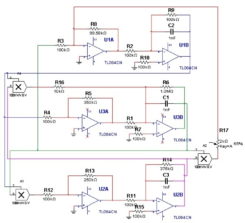
Figure 1: Basic electronic circuit which models Eqs (2.2). Nominal values of resistors and capacitors are shown on the scheme. The analog multipliers (denoted by crosses) are of the type AD633AN. Variables $u,v,w$ are output voltage values of operational amplifiers U1B, U2B and U3B, respectively.

The cited values of electrical characteristics correspond to fixed values $\sigma=10$ and $b=8/3$ in Eqs (2.2). Changing of parameters $A$ and $R$ is enabled by variation of respective resistances R17 and R5. The value of $A$ equals 10 divided by the value of R17 in $k\Omega$; the value of $R$ equals 0.01 of the resistance R5 in $k\Omega$.

To ensure that all voltages in the circuit stay inside the operating range of dynamical multipliers (from –10 to 10 V), the original dependent and independent variables need to be rescaled: we assume that the dimensionless potential differences $x$, $y$ and $z$ are measured in volts, and proceed to $u=x/5$, $v=y/5$, $w=z/10$. For the time measured in “seconds”, we introduce $\tau=t/T$ with $T$=100. This recasts Eqs (2.2) into

$$u^{\prime} = T\left(\sigma(v-u)+10\,A\,v\,w\right)$$

$$v^{\prime} = T\,(R\,u-\,v\,-\,10\,u\,w)$$ (3)

$$w^{\prime} = T\,(2.5\,u\,v\,-b\,w)$$

where prime denotes differentiation with respect to $\tau$. Finally, it should be noted that, due to inevitable presence of nonlinearities in the multipliers, the real circuit, in fact, does not reproduce the perfect symmetry of Eq.(3) with respect to the simultaneous change of sign of voltages $u$ and $v$.

In order to initiate the trajectories close to the unstable manifold of the saddle point, the circuit was grounded for a short time. The subsequent growth of voltage began from rather small values.

Voltages were measured and recorded at a rate of 5000 records per second. We did not apply any kind of filtering; stability of the scheme and smallness of time-step allowed us to plot quite smooth phase portraits of the system directly from the experimental data.

4 Results

4.1 Lorenz scenario of transition to chaos

We measured and recorded time-dependent voltages in the circuit for various values of the parameters $A$ and $R$ at fixed $\sigma$=10 and $b$=8/3. The equilibrium $u$=$v$=$w$=0 is stable for $R<$1 and is a saddle-point in the range $R>$1. Measurements on the circuit and numerical integration of Eqs (2.2) confirm existence of the curve $R_{\rm hom}(A)$ upon which principal homoclinic orbits to this saddle are formed. Both in the experiment and in numerical studies this event is marked by change in the asymptotics of large $t$ for trajectories with initial conditions near the origin. Prior to the bifurcation, the trajectory which starts with small positive values of $u$ and $v$ tends to the attractor (equilibrium or oscillatory state) which is contained in the half-space $u>0$. After the bifurcation, this trajectory makes a loop in the half-space $u>0$, crosses into the opposite half-space $v<0$ and settles on the attractor there.

Under low values of $A$, formation of homoclinic orbit occurs at $\nu<1$; this corresponds to the Lorenz scenario of transition to chaos. Immediately beyond this curve the chaotic set, created by the homoclinic explosion at $R_{\rm hom}(A)$, is unstable; its presence is reflected in the existence of chaotic transients which precede relaxation to stable equilibria (“metastable chaos” [27]). On the parameter plane, the domain corresponding to this kind of dynamics is bounded from above by the curve $R_{\rm ch}(A)$ which marks stabilization of the chaotic set and emergence of the chaotic attractor. Upon this curve the unstable manifold of the saddle point hits the stable manifold of the unstable periodic orbit [5]. Numerically, we detected the latter curve by tracking the separatrices of the saddle point; in the experiments $R_{\rm ch}(A)$ was identified as the lowest value of $R$ (or the leftmost value of $A$) where the circuit possessed non-decaying chaotic dynamics. For values of $R$ beyond $R_{\rm ch}(A)$, we observed irregular oscillations of voltages, with phase portraits strongly reminiscent of the Lorenz attractor (Fig. 2).

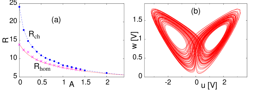
Figure 2: Lorenz-like dynamics at $\nu<1$ with $\sigma$=10 and $b$=8/3.
(a): Bifurcations on the parameter plane. Solid line $R_{\rm hom}$ (numerics), and crosses (experiment): homoclinic explosion. Dashed line $R_{\rm ch}$ (numerics) and circles (experiment): onset of chaotic motion. (b): Projection of the phase portrait at $A$=1.5, $R$=3.6 (experiment).

4.2 Sequences of gluing bifurcations

According to the above reasoning, homoclinic explosion should be replaced by the gluing bifurcation when the corresponding value of $R_{\rm hom}$ gets below $R_{\nu}$=209/45=4.6444$\ldots$; this corresponds to the range $A\geq$ 4. Indeed, we observed in the experiment the Lorenz-like chaotic attractors for $A<4$ and gluing bifurcations for $A>4$.

We illustrate the transformation of the phase portrait along the gluing bifurcation scenario with the plots of projections which correspond to increase of $A$ at constant values of other parameters.

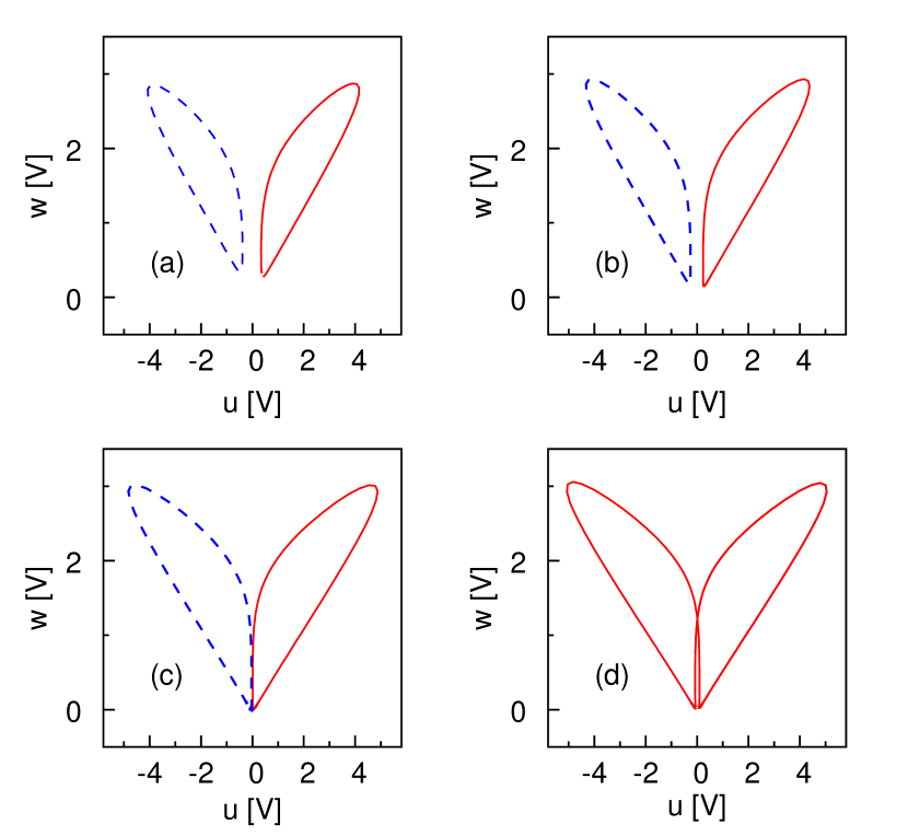
Figure 3: Principal gluing bifurcation in the circuit: Evolution of the attracting set. Parameter values: $\sigma$=10, $b$=8/3, $R$=3.6.
(a): $A$=6.4; two stable periodic orbits. (b): $A$=6.55; two stable periodic orbits. (c): $A$=7.; formation of two trajectories, homoclinic to the equilibrium. (d): $A$=7.05; stable self-symmetric orbit with two loops.

By varying initial conditions, we are able to identify in the phase space of the circuit two attracting closed trajectories which are almost symmetric to each other (Fig.3a). As the parameter $A$ is increased, these two orbits come closer (Fig.3b), approach the invariant manifolds of the saddle equilibrium at the origin and form the pair of symmetric homoclinic orbits to this saddle (Fig.3c). A slight increase of the parameter $A$ makes the homoclinic orbits break up and disappear: the only attractor of the system, plotted in Fig.3d, is the periodic orbit with two loops which is (up to instrumental resolution) invariant under the symmetry transformation $\{u\to-u$, $v\to-v\}$ . Close to the homoclinic bifurcation, the measured values of the period $T_{0}$ of the oscillations match the known logarithmic asymptotics: $T_{0}(A)\sim-\log(A_{\rm hom}-A)$.

As seen in Fig.4, the oscillations are strongly anharmonic: the overwhelming part of the period is spent in nearly motionless state. This corresponds to long hovering of the trajectory in the vicinity of the saddle point.

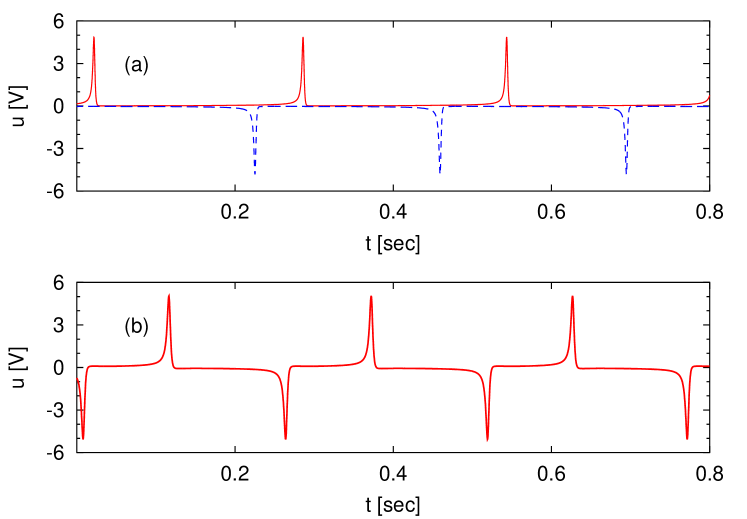
Figure 4: Temporal evolution close to the gluing bifurcation.
(a): $A$=7.0; oscillations on limit cycles with 1 loop prior to the bifurcation. (b): $A$=7.05; oscillations on the limit cycle with 2 loops. Other parameters like in Fig. 3.

Further stages of the evolution of the attracting trajectory are sketched in Fig.5. The symmetric limit cycle with two turns (Fig.3d) loses stability as a result of the pitchfork bifurcation. One of the two resulting stable asymmetric limit cycles is shown in Fig.5a. As the parameter is further increased, these two limit cycles approach the invariant manifolds of the equilibrium, and the secondary gluing bifurcation takes place: two homoclinic orbits with 2 turns are formed. Their subsequent breakup produces a single symmetric stable orbit with 4 turns (Fig.5b). Further, the events are repeated on the new level: the symmetric orbit with 4 turns is destabilized, and two stable asymmetric ones are born (Fig.5c). These asymmetric periodic orbits merge in the next gluing bifurcation, form a pair of homoclinic orbits with 4 turns, and leave the stable periodic orbit with 8 turns, shown in Fig.5d.

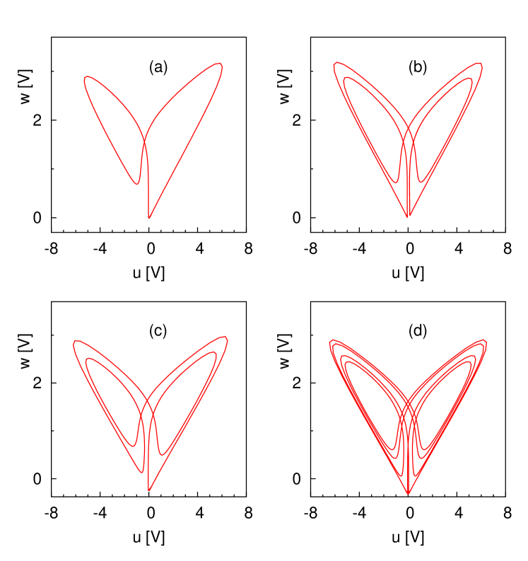
Figure 5: Further stages of the gluing scenario (parameters: $\sigma$=10, $b$=8/3, $R$=3.6). (a): $A$=8.05; asymmetric stable periodic orbit with two turns (b): $A$=8.10; symmetric stable periodic orbit with 4 turns, born from the secondary gluing bifurcation. (c): $A$=9.37; asymmetric stable periodic orbit with 4 turns; (d): $A$=9.38; symmetric stable periodic orbit with 8 turns, born from the third gluing bifurcation.

In the perfectly symmetric setup this bifurcation sequence would continue, each time doubling the number of turns of the attracting periodic orbit in the phase space [16]. Presence of asymmetry is known to disable the complete sequence of homoclinic “doublings” [28, 29]; mathematically, this owes to the fact, that linearization of the corresponding renormalization operator near its fixed point possesses an additional unstable direction, responsible for the asymmetry. Finite resolution of our measurements (finite step-size for variable resistance R17 in Fig. 1) as well as the inevitable asymmetry in the electronic circuit did not allow us to resolve the further stages of the gluing process: instead we observe rapid emergence of the chaotic attractor (top row of Fig. 6).

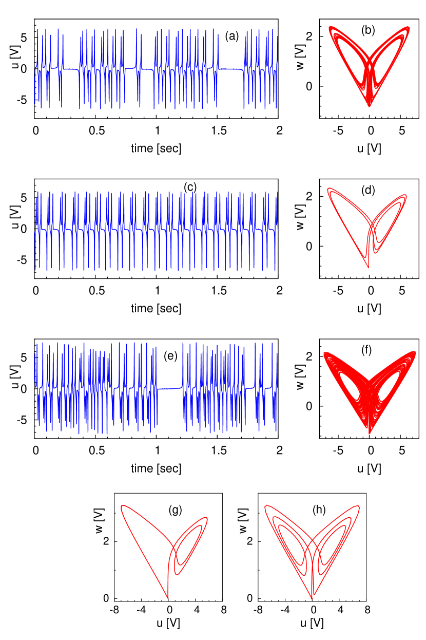
Figure 6: Experimental records of dynamics beyond the first gluing sequence. (a,b): Chaotic attractor at $A$=9.39. (c,d): Limit cycle with 5 turns at $A$=10.17. (e,f): Chaotic attractor at $A$=13.46. (g,h) gluing bifurcation, mediated by homoclinic orbits with 3 turns at $A$=11.51. Other parameters: $\sigma$=10, $b$=8/3, $R$=3.6.

A characteristic feature of chaotic oscillations in this circuit, well recognizable in the oscillograms of Fig. 6(a,e), is presence of relatively long nearly quiescent plateaus: they correspond to hovering near the saddle point. Further increase of the parameter $A$ has disclosed that the range in which oscillations are chaotic, is interspersed by numerous windows in which various stable symmetric and asymmetric periodic oscillations are observed. One of such periodic states is shown in Fig. 6(c,d). In terms of the parameter $A$, periodic windows are bounded from above by secondary homoclinic bifurcations and serve as starting states of further gluing scenarios. An example of bifurcation, in which two periodic regimes with three turns glue together and create a periodic orbit with six turns is shown in Fig. 6(g,h). It should be noted, that increase of the resistance R17 enhances asymmetry in the circuit, therefore, in general, homoclinic trajectories formed, respectively, by the “left” and the “right” components of the unstable manifold occur at slightly different values of the parameter $A$.

5 Discussion and Outlook

We have demonstrated in the experiment on the analog electronic circuit the Lorenz scenario of transition to chaos as well as several initial stages of the sequence of gluing bifurcations. The circuit mimics the modified Lorenz system, and we utilized the fact that modification allows, by variation of a single resistance, to move across the parameter space without changing the value of the saddle index. Observed sequence of transformations of phase portraits provides an unambiguous qualitative confirmation of theoretical predictions. For a quantitative comparison (convergence rate of the bifurcation scenario and other scaling constants), the experimental resolution – in particular the step-size of the active parameter – should be improved.

In a wider context of dynamical systems with gluing bifurcations, it should be noted that a straightforward coding procedure maps temporal evolution of voltages onto the binary alphabet: a symbol 1 is assigned to each turn of the orbit in the half-space $u>0$, and a symbol 0 marks each turn in the half-space $u<0$. In this sense, a pair of binary codes which correspond to two components of the unstable manifold of the saddle, provides a complete characterization of dynamics [19]. In presence of symmetry, one code is sufficient; remarkably, it is related to the kneading sequence of the family of logistic mappings. In case of noticeable asymmetry, both kneading sequences are needed; here, certain aspects of the description are analogous to the formalism for (in general, discontinuous) circle mappings: rotation numbers, devil staircase etc. [21]. Since our experimental results match well the theoretical description of the route to chaos for symmetric systems, we may hope that explicit introduction of controlled asymmetry into equations (3) and into the analog circuit of Fig. 1 should allow to detect in the circuit bifurcation also those scenarios which theory predicts for asymmetric gluing bifurcations.

References

References

- [1] H. G. Schuster, Deterministic Chaos, An Introduction, VCH – Verlag, Weinheim, 1988.
- [2] J. Argyris, G. Faust, and M. Haase, An Exploration of Chaos, North-Holland, Amsterdam, 1994.
- [3] E. N. Lorenz, J. Atmos. Sci., 20, 130 (1963).
- [4] C. Sparrow, The Lorenz Equations: Bifurcations, Chaos, and Strange Attractors, Springer, Berlin, 1982.
- [5] V. S. Afraimovich, V. V. Bykov, and L. P. Shilnikov, Sov. Phys. Doklady 22, 253 (1977).
- [6] J. M. Gambaudo, P. Glendinning and C. Tresser, Nonlinearity 1 203 (1988).
- [7] D. V. Lyubimov and M. A. Zaks, Physica D 9, 52 (1983).
- [8] F. H. Busse, M. Kropp, and M. Zaks, Physica D 61, 94 (1992).
- [9] A. M. Rucklidge, Nonlinearity 6, 1565 (1994).
- [10] G. Demeter and L. Kramer, Phys. Rev. Lett. 83, 4744 (1999).
- [11] V. Carbone, G. Cipparrone, and G. Russo, Phys. Rev. E 63, 051701 (2001).
- [12] R. Herrero, J. Farjas, R. Pons, F. Pi, and G. Orriols, Phys. Rev. E 57, 5366 (1998).
- [13] J. Abshagen, G. Pfister, and T. Mullin, Phys. Rev. Lett 87, 224501 (2001).
- [14] P. K. Roy and S. K. Dana, Int. J. Bifurcation Chaos 16, 3497 (2006).
- [15] L. P. Shilnikov, Mat. Sbornik 61 (103), 443 (1963).
- [16] A. Arneodo, P. Coullet, and C. Tresser, Phys. Lett. A 81, 197 (1981).
- [17] A. S. Pikovsky, M. A. Zaks, U. Feudel, and J. Kurths, Phys. Rev. E , 52, 285 (1995).
- [18] J.-M. Gambaudo, I. Procaccia, S. Thomae, and C. Tresser, Phys. Rev. Lett 57, 925 (1986).
- [19] I. Procaccia, S. Thomae, and C. Tresser, Phys. Rev. A 35, 1884 (1987).
- [20] D. V. Lyubimov, A. S. Pikovsky, and M. A. Zaks, in Mathematical Physics Review, vol.8, edited by S. P. Novikov (Gordon and Breach, Chur, 1989), pp. 221–292.
- [21] M. A. Zaks, Physica D 62, 300 (1993).
- [22] L. A. Sanchez, J. Differential Equations 217, 341 (2005).
- [23] P. Yu, X. Liao, Int. J. Bif. Chaos 16, 757 (2006).
- [24] G. A. Leonov, Phys. Lett. A 376, 3045 (2012).
- [25] G. A. Leonov, Int. J. Bif. Chaos 23, 1350058 (2013).
- [26] E. Sanchez, M. A. Matias, Phys. Rev. E 57, 6184 (1998).
- [27] J. A. Yorke, E. D. Yorke, J. Stat. Phys. 21, 263 (1979).
- [28] P. Collet, P. Coullet, C. Tresser, J. Physique Lett. 46, 143-147 (1985).
- [29] M. A. Zaks, Phys. Lett. A 175, 193 (1993).