Weighted statistical parameters for irregularly sampled time series
Abstract
Unevenly spaced time series are common in astronomy because of the day-night cycle, weather conditions, dependence on the source position in the sky, allocated telescope time, corrupt measurements, for example, or be inherent to the scanning law of satellites like Hipparcos and the forthcoming Gaia. Irregular sampling often causes clumps of measurements and gaps with no data which can severely disrupt the values of estimators. This paper aims at improving the accuracy of common statistical parameters when linear interpolation (in time or phase) can be considered an acceptable approximation of a deterministic signal. A pragmatic solution is formulated in terms of a simple weighting scheme, adapting to the sampling density and noise level, applicable to large data volumes at minimal computational cost. Tests on time series from the Hipparcos periodic catalogue led to significant improvements in the overall accuracy and precision of the estimators with respect to the unweighted counterparts and those weighted by inverse-squared uncertainties. Automated classification procedures employing statistical parameters weighted by the suggested scheme confirmed the benefits of the improved input attributes. The classification of eclipsing binaries, Mira, RR Lyrae, Delta Cephei and Alpha2 Canum Venaticorum stars employing exclusively weighted descriptive statistics achieved an overall accuracy of 92 per cent, about 6 per cent higher than with unweighted estimators.
keywords:
methods: data analysis – methods: statistical – stars: variables: general.1 Introduction
Unevenly sampled astronomical time series are common in both ground- and satellite-based observations, and typically include time intervals with clustered and scattered data. For example, the sampling laws of surveys such as the Hipparcos111http://hipparcos.esa.int (ESA, 1997; Perryman et al., 1997) and the forthcoming Gaia222http://gaia.esa.int (Perryman et al., 2001) missions are characterized by gaps and clumps of measurements on time-scales much greater and smaller than the average sampling interval, respectively.333In the case of the Hipparcos data, sources were typically observed in sequences of 4 to 6 transits separated by 20 and 108 min and repeated every 3 to 5 weeks (Eyer et al., 1994).
A significant number of studies were devoted to the estimation of power spectra and modelling of irregularly sampled time series (e.g., Carbonell, Oliver & Ballester, 1992; Koen, 2005; Vio, Strohmer & Wamsteker, 2000). Various theoretical approaches to the problem of estimating the true values of irregularly sampled signals are described in the literature (e.g., Rybicki & Press, 1992; Scargle, 1989, 1990). This paper evaluates pragmatically the effectiveness of some of the simplest solutions which can be implemented in a pipeline to process extremely large data volumes. Big data constitute one of the current challenges in astronomy, with surveys like Gaia, the Panoramic Survey Telescope & Rapid Response System444http://pan-starrs.ifa.hawaii.edu/public (Pan-STARRS, Kaiser et al., 2002) and the Large Synoptic Survey Telescope555http://www.lsst.org/lsst (LSST, Ivezić et al., 1994), among others, which require efficient algorithms to produce results that are as accurate as possible. Considering that per-cent level improvements can impact on decisions of a very large number of sources, tuning the balance between efficiency and accuracy is an important task of data processing.
The objectives of the present study are statistical parameters (like moments and percentiles) of time series of deterministic signals. If linear interpolation in time or phase is able to describe major features of signals, simple recipes can improve the accuracy of statistical parameters and that of subsequent analyses such as automated classification. The effect of the latter is tested on data related to periodic variable stars from the Hipparcos mission, which is one of the closest proxies for the sampling of Gaia (for which the improvement of a few per cent in classification accuracy can increase by millions the number of correctly classified variable sources).
The parameters considered for better accuracy include descriptive statistics such as the mean, variance, higher central moments and robust equivalents: they can summarize essential features of signals in a few numbers employing straightforward computations, which makes them excellent precursors of more detailed analyses like modelling and classification. Herein, a simple recipe to mitigate the effects of irregular sampling on the characterization of a signal in terms of statistical parameters is presented. Separate works describe corrections of biases induced by small sample sizes and Gaussian uncertainties in the calculation of weighted moments and cumulants (Rimoldini, 2013a, b).
Time series sampled irregularly or with varying candences may lead to very different estimates of statistical parameters for the same signal. For example, if a sinusoid is sampled mostly at maximum or minimum, the mean is offset by about the amplitude of the signal, the variance might be much smaller than expected (since most points sample the same region of the signal), and the distribution appears very skewed (the few non-clumped measurements form an asymmetric tail in the distribution of measurements). If the same clump of data was in proximity of the average level, instead, the mean and skewness values could be close to the correct value (by serendipity), but the variance would be much smaller than the true one.
Sampling-induced biases do not arise from sparsely sampled data only and they might manifest independently of the number of measurements. While time series with more measurements are generally associated with better coverage of signal features, the importance implicitly assigned to different parts of the signal by unweighted estimators is related to the relative frequency of measurements.
In principle, the most accurate and precise statistical parameters could be inferred from the model of a signal. Alas, models are often complicated, in the attempt to describe the signal features under many circumstances, they might require lengthy processing and their accuracy cannot be guaranteed in all cases. For example, Fourier series are well fitted to model periodic signals, but the description of sharp features, like those present in EA-type eclipsing binaries, requires a high number of harmonics, which can overfit smoother parts of the signal and cause unrealistic excursions in large intervals with no data (Dubath et al., 2011).
Linear interpolation is one of the simplest methods to approximate a model, assuming the signal features are sufficiently sampled. This work estimates statistical parameters by averaging the linear interpolation of functions of time series measurements (depending on the specific estimator). If the signal can be recognized in time domain, interpolation can be performed in time without requiring further information. If a sparsely sampled signal is primarily mono-periodic, it can be interpolated in phase by folding the time series with the corresponding period. While the interpolated function might include profiles with spiky artefacts, its average is more robust and can be expressed as a weighted mean which assigns more relevance to scattered than clumped measurements. Statistical parameters weighted by such a scheme were tested on data from the Hipparcos periodic catalogue and led to a significant general improvement in the accuracy and precision of estimator values and automated classification results, with respect to those obtained with the unweighted or error-weighted counterparts.
This paper is organized as follows. After the definition of the notation and terminology in Sec. 2, the description of weighted estimators as averages of linear interpolations is presented in Sec. 3, with weights defined in time and phase, including adaptations for low signal-to-noise regimes and small sample sizes. The new weighting scheme is applied to time series from the Hipparcos periodic catalogue in Sec. 4, which includes a comparison of the values of statistical parameters computed with different weighting schemes and their effect on automated classification. The conclusions are drawn in Sec. 5, followed by a series of appendices with more details on the interpolation of (mono-)periodic signals (Appendix A), the illustration of modelled light curves to verify the accuracy of estimators (Appendix B), the definitions of the statistical parameters employed (Appendix C) and additional scatter plots of estimators (Appendices D and E).
2 Notation and terminology
For a set of measurements , the following quantities are defined:
-
(i)
The population central moments of order around the mean are denoted by and respective cumulants , and (e.g., Stuart & Ord, 1969).
-
(ii)
Sample weighted central moments are defined in terms of weights as , with respective cumulants , where and .
-
(iii)
Standardized skewness and kurtosis are and , with population values and , respectively.
-
(iv)
Noise-unbiased estimates (sometimes called ‘denoised’ for brevity) of central moments and cumulants (Rimoldini, 2013b) are denoted by an asterisk superscript.
-
(v)
No systematics or instrumental errors are considered herein and uncertainties are often referred to as errors.
-
(vi)
The accuracy of an estimator is related to its distance from the true value and thus combines the concepts of bias and precision, while the classification accuracy rate is the ratio between the number of true positives and the total number of stars (of a given type).
-
(vii)
The precision of an estimator is quantified by its dispersion, while the classification precision rate is the ratio between the number of true positives of a given type and the total number of stars classified as such a type.
3 Method
The proposed weighting scheme is derived from linear interpolation and thus all of its pros and cons are inherited by definition. In particular, applications are limited to deterministic signals and the characterization of stochastic processes is excluded. Considering the great variety of signal shapes and sampling laws, simulations are suggested to better assess the accuracy gains and losses of the method based on a representative subset of the data and estimators under consideration, as illustrated in Sec. 4. Strictly speaking, statistical estimators like the mean and moments are not defined for deterministic signals. However, such estimators can still give acceptable approximations when the time scale of features (or period) is much smaller than the time series duration. In the case of mono-periodic signals, the proposed weighting scheme leads to estimator values of the signal as if the latter was measured on a complete cycle.
Herein, the targeted (population) value of a generic statistical parameter of a continuous deterministic signal in time is computed by integrating the estimator function of such a signal over the time series duration :
| (1) |
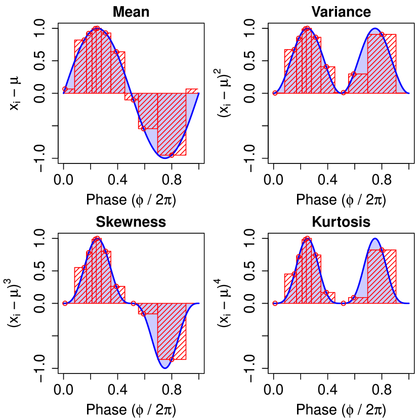
where is a function of the signal at a given time . For example, in the case of a periodic source, time can be replaced by phase and is represented by the mean areas shaded in blue in Fig. 1. In the case of regular sampling in fine intervals, replacing the integration with the sum of discrete elements tends to the population result for infinitely small intervals. This limit is not necessarily satisfied when a continuous signal is sampled irregularly. The weighting scheme described in Sec. 3.1 recovers the property that the sum of discrete (weighted) terms approaches the result of the continuous function, in the limit of very dense (although not necessarily uniform) sampling.
Linear interpolation is a simple method to approximate a function with a broken line connecting the data points, provided the function is sufficiently sampled in time or phase. In this section, such a function is represented by the expression of the additive terms of a statistical estimator. For example, a central moment of order is defined by the average of terms of the form . Results from linearly interpolating such a function are equivalent to those obtained from an effectively infinite regular sampling of the interpolated function. In Sec. 3.1, it is shown that the average of a linear interpolation in time or phase can be expressed as a weighted mean. For example, central moments of a sinusoidal signal are illustrated in Fig. 1 and they are related to the areas enclosed by , which are approximated by terms (corresponding to the heights of bars) with weights (related to the widths of bars) adapting to the sampling density in phase.
Weighting can decrease the effective sample size, since more importance is given to some measurements at the expense of other ones (e.g., a large sample with only a few important elements will be similar to one with only these few elements) and exploiting correlations in the data with weights (e.g., assigning small weights to measurements separated by small intervals because their values are expected to be similar) might introduce biases if applied to expressions assuming independent data. However, small biases could be justified by significant improvements in precision and a mixed weighting scheme which balances precision and accuracy depending on the signal-to-noise () level and sample size is described in Sec. 3.1.3.
3.1 Weighting schemes
If the targeted features of signals are sufficiently sampled in time, as for the data from the Kepler (Borucki et al., 2010) and CoRoT (Auvergne et al., 2009) missions, linear interpolation is expected to provide reliable approximations of most deterministic signals and weights might be expressed in time domain (see Sec. 3.1.1). If typical time intervals between measurements are larger than the resolution needed to sample the signal (as it is often the case in the Hipparcos and Gaia surveys) but the latter is mono-periodic or dominated by a single period, sampling can be improved by folding the light curve with the value of the fundamental period and computing interpolations (or weights) in phase (see Sec. 3.1.2).
The interpolation-based weighting scheme naturally removes importance from clumped data (oversampling the same region of the signal) in favour of more scattered measurements (probing extended parts of the signal). If gaps in time or phase occasionally cover a relevant fraction of a signal, measurements at the gap boundaries might not provide sufficient information on the features of the signal and the importance of such data could be limited, for example, to some maximum weight value. This strategy can extend the applicability of the weighting scheme described in Sec. 3.1.1 to under-sampled deterministic signals, periodic or non-periodic, to mitigate statistical biases due to data clumps on scales smaller than the signal features aimed at. For example, rare stellar bursts of short duration are expected to be associated with a skewed distribution of magnitudes. If sampling happens to be denser during one of the bursts, the value of the skewness can differ strongly, while appropriately weighting dense measurements could alleviate the problem.
3.1.1 Weights in time
If an estimator is defined by the average of a function in time as in Eq. (1), it can be approximated by the mean of the linear interpolation of terms at times , where for a time series of measurements sorted in time, and it can be expressed as a weighted average as follows:
| (2) | ||||
| (3) | ||||
| (4) | ||||
| (5) | ||||
| (6) |
where
| (7) | |||
| (8) | |||
| (9) |
and
| (10) |
When differences between successive times are too large for sensible interpolation, they might be limited to some maximum interval as follows:
| (11) | ||||
| (12) | ||||
| (13) |
and, of course, then .
3.1.2 Weights in phase
If sampling in time is sparse but the data exhibit periodicity, the time series can be folded with the dominant period to increase the average sampling rate in phase (by a factor of the order of the duration of the time series divided by the period).
3.1.3 Examples of mixed weighting schemes
In order to avoid interpolating large noise fluctuations, weights could be set to reduce to inverse-squared uncertainties at low , which proved more precise in the simulations described by Rimoldini (2013b). The transition between high and low regimes could be pursued with weights of the form
| (17) |
where and denote the uncertainty and interpolation-based weight (introduced in the preceding paragraphs) associated with the -th measurement, respectively, and
| (18) |
The family of functions defined in Eq. (18) is only one example of many possible alternatives with the same limit behaviours. The dependence on the ratio and a set of tuning parameters (such as ) make it possible to control a mixed weighting scheme and in particular regulate the transition of weights from to in the limits of high and low ratios, respectively. In the same spirit, a further function of the form could be used to reduce the relevance of interpolation-based weights for small sample sizes (as alternative to weights limited by maximum interpolation intervals):
| (19) |
where is defined by Eqs (7)–(9) or (26)–(28). Tuning parameters offer the possibility to reach a compromise solution between precision and accuracy at high and low values of and ratios, according to the specific set of estimators, signals, sampling, errors, sample sizes and their distributions in the data. The determination of such parameters might involve the maximization of the overall accuracy of the set of estimators under consideration, employing data simulated in a context similar to the one intended for analysis. The effect of such tuning parameters on simple simulated signals is illustrated in Rimoldini (2013a, b) as a function of sample size and ratio, while an application to real data is presented in the next section.
4 Hipparcos periodic variable stars
The effect of interpolation-based weights on statistical parameters was explored for a realistic distribution of signals, represented by time series from the Hipparcos catalogue of periodic variable stars. The Hipparcos mission (ESA, 1997) performed astrometric and photometric measurements of the brightest sources in the sky. The full catalogue (Perryman et al., 1997) contains 118 204 sources with photometry. Among the 11 597 stars identified as variables, a reliable period could be computed (or was consistent with the one from literature) for 2 712 objects, which were published in the periodic catalogue (Vol. 11 ESA, 1997; Eyer, 1998). This set of sources, which contained light variations dominated mostly by single periods, was chosen to illustrate the application of one of the weighting schemes described in Sec. 3.
4.1 Statistical parameters
In order to assess the accuracy of estimators with respect to the (unknown) real signal, the latter was assumed to be represented by a model of the time series and the magnitude measurements were simulated employing the true uncertainties as Gaussian random variables (around the model) at the phases given by the real data. Only good quality measurements were accepted, flagged by the field HT4 as zero or one (see Vol. 1 of ESA, 1997), which reduced the number of sources considered to 2683.666The Hipparcos identifiers of sources with no good quality measurements (i.e., with field HT4 only) were: 1196, 10027, 17878, 20570, 24019, 25673, 39084, 42715, 42726, 46502, 52538, 53937, 58112, 60904, 61997, 63125, 69582, 72583, 88905, 90026, 93595, 93724, 96007, 99675, 102246, 102409, 112317, 112470 and 118188.
4.1.1 Light-curve models
Time series were folded with the period provided by the Hipparcos catalogue777The mean period (field P11 of ESA, 1997) derived from the Hipparcos data was employed. If this was not available, the period from the literature (listed in field P18) was considered. and modelled by a cubic smoothing spline (the smooth.spline function from the stats package in R, R Development Core Team, 2013). The condition of periodicity at the boundaries was approximated by replicating a whole cycle of folded data before and after the cycle considered as reference for the ‘true’ statistical parameters and for the generation of simulated data. The smoothing parameter was estimated from the data with a generalized cross-validation method (e.g., Ruppert, Wand, & Carroll, 2003) and the degrees of freedom were adjusted in special cases, to mitigate over-fitting highly clumped data with large gaps as well as under-fitting the profile of eclipsing binaries.888The number of degrees of freedom df depended on the unweighted standardized sample skewness of the data, which identified light variations typical of eclipsing binaries, and the ratio between the median and the third largest gaps in phase, to better deal with clumped data with large gaps. Denoting by the number of measurements in a time series, df equalled 15, 24 and 36 for less than , and , respectively, provided . For greater values of , df was set to the smallest integer not less than . The quoted values of df take into account the replicated data at each of the extremes of the folded light curve (to induce quasi-periodic boundary conditions on the model of the central cycle). The combination of large gaps and sharp features did not lead to accurate models and other methods might help avoid modelling artefacts in gapped data, although these are out of the scope of this application. Also, cases in which sparse sampling missed important features could not be improved. Nevertheless, the smoothed best-fitting curves seemed to capture the relevant shapes of true signals in most cases.
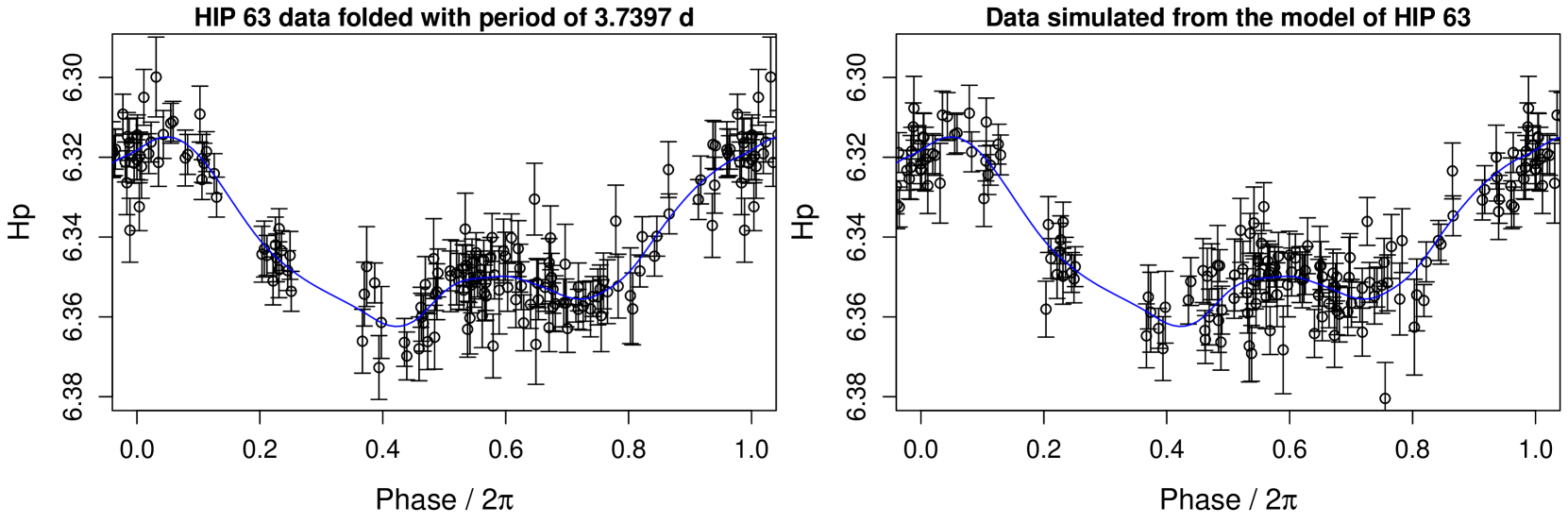
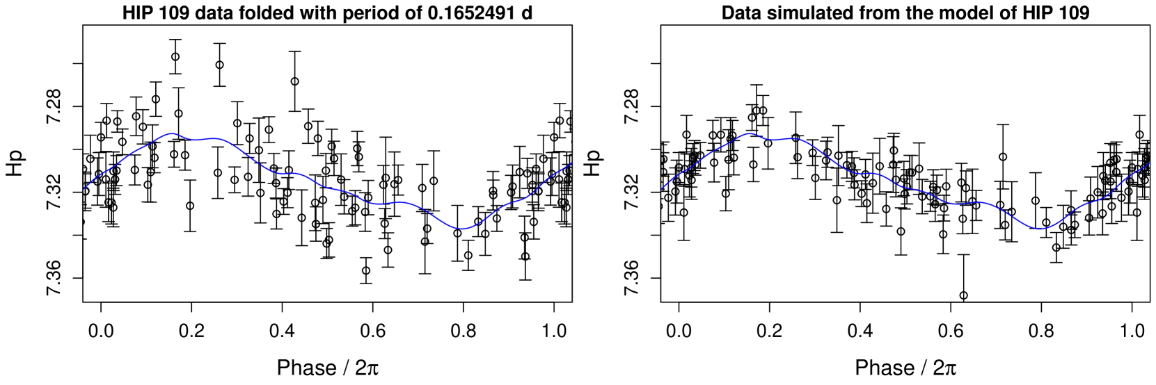
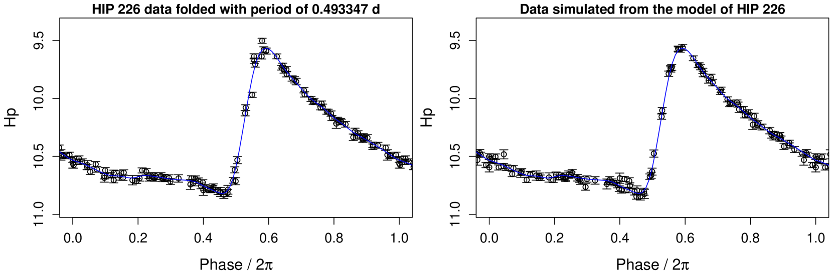
The resulting models are presented together with the original and simulated data in Appendix B. The difficulty to achieve accurate models for all sources and the need of more complex modelling techniques were confirmed. While models were sometimes not ideal, most of them were of sufficient quality to supply a realistic distribution of the relevant features of the Hipparcos periodic variable stars. Differences from data of other surveys were expected to be greater than those due to modelling inaccuracies. Less than one per cent of all sources (23 time series)999The Hipparcos identifiers of the 23 sources removed from consideration because of poor modelling were: 1901, 4279, 21600, 23416, 23453, 25591, 32397, 40853, 42853, 45094, 48054, 58854, 61281, 68064, 73533, 76152, 89579, 90313, 95611, 96739, 104483, 108317 and 112928. with significant modelling artefacts in gaps with no data were removed (many of them were EA-type eclipsing binaries with large data gaps), thus 2660 objects were included in the assessment of statistical parameters. The number of measurements per time series ranged from 18 to 331, with ratios from 0.2 to 116, according to the definition in Eq. (20).
4.1.2 Weighting scheme
The Hipparcos light curves were folded with the catalogue period and interpolation-based weights were computed in phase. For brevity, such weights are referred to as ‘phase weights’, while inverse-squared uncertainties are called ‘error weights’.
The estimators employed herein included weighted moments and cumulants corrected for biases from Gaussian uncertainties (called ‘noise-unbiased’ or ‘denoised’ estimators; see Rimoldini, 2013b) and some robust weighted measures, as defined in Appendix C. Simulations in Rimoldini (2013a, b) suggested that noise-unbiased phase-weighted sample moments can be more accurate for and sample sizes with respect to other schemes, while error weighting appeared the most appropriate option for noisy signals. Thus, the weighting scheme chosen for this application combined error and phase information as described by Eqs (17) and (26)–(28). The balance between phase weights (at high ) and error weights (at low ) was controlled by the parameters and , which provided a satisfactory overall accuracy for the set of estimators and light-curve shapes of the Hipparcos periodic variable stars. The signal-to-noise ratio was estimated from the true (model) signal variance and the average of squared measurement uncertainties as follows:
| (20) |
4.1.3 Results
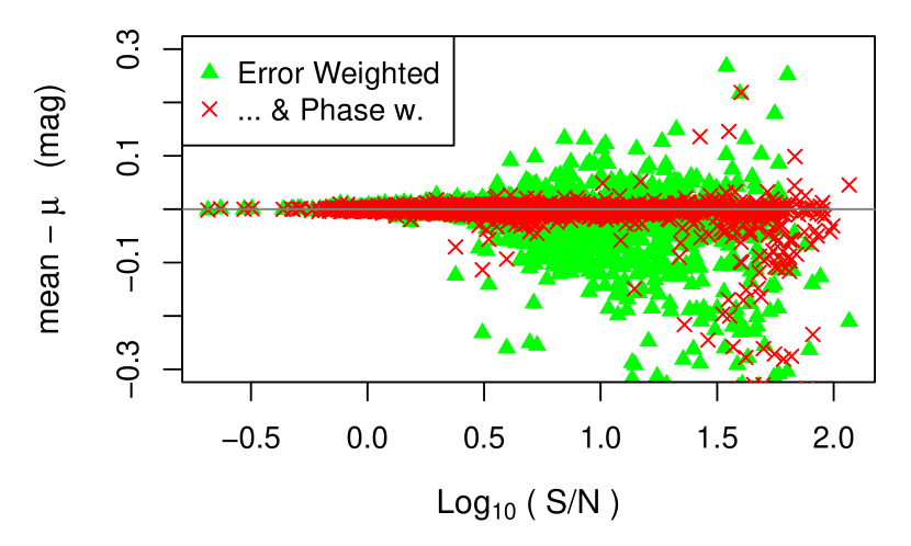
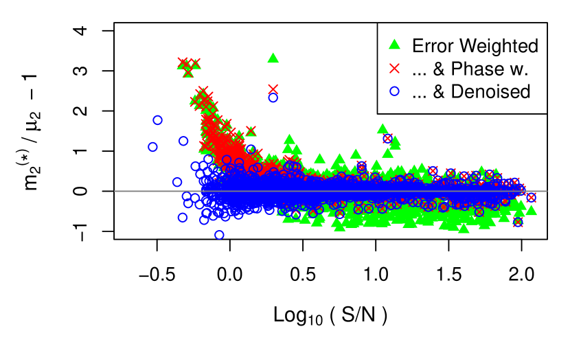
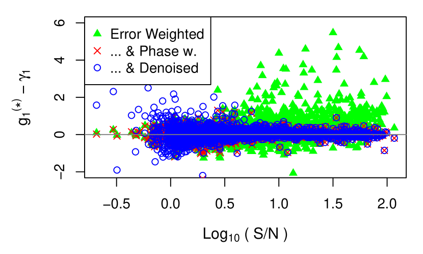
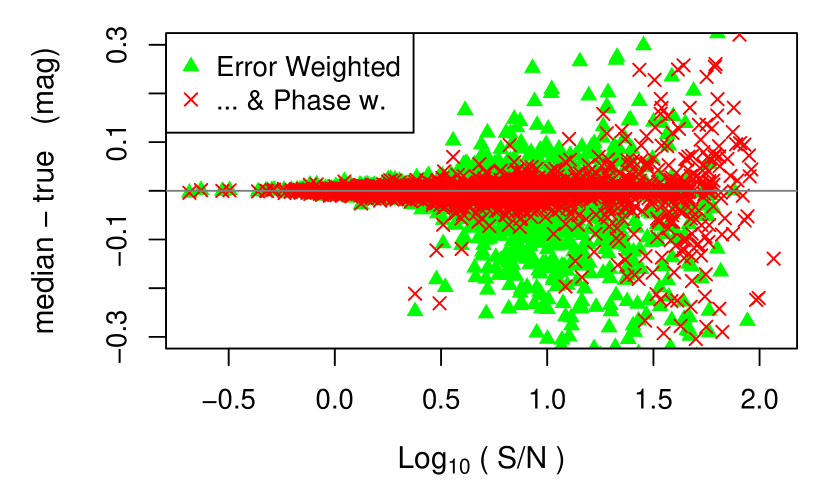
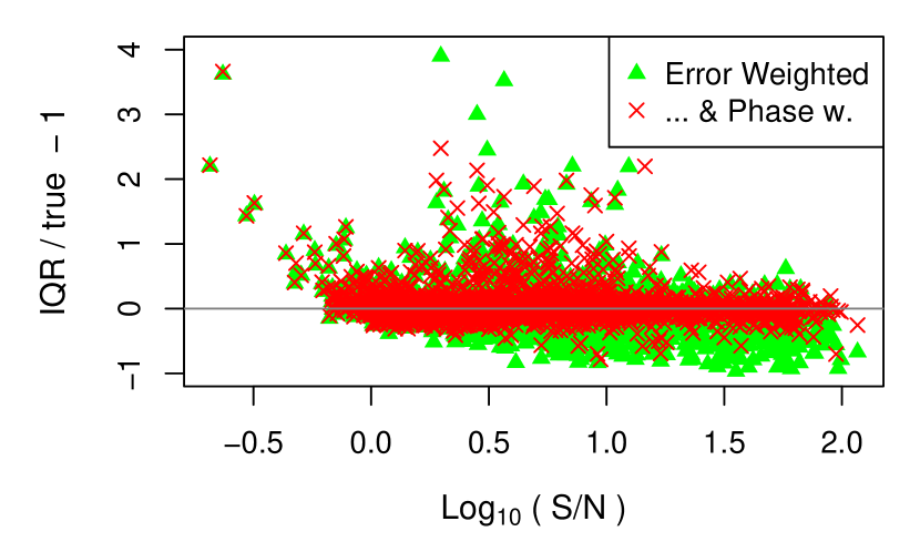
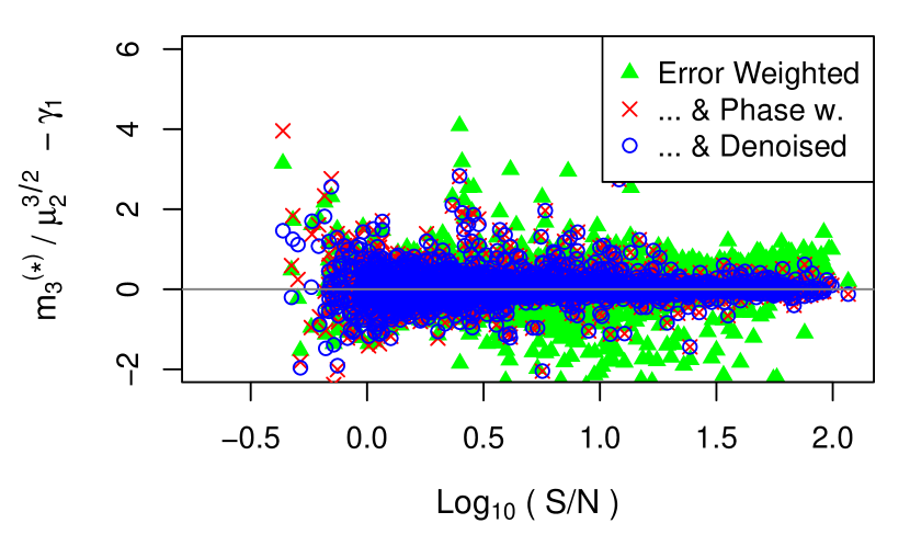
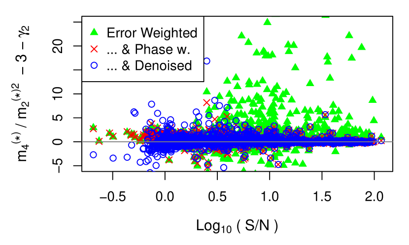
The deviations of error-weighted sample statistical parameters from population values (computed from a fine regular sampling of the models) are compared to the noise-unbiased error-phase weighted counterparts as a function of ratio in Figs 2–3. Error-phase weighted (and noise-unbiased, when applicable) estimators were generally more accurate than error-weighted estimators. Since larger light variations were correlated with higher levels, the effect of the correlation between errors and magnitudes (e.g., see van Leeuwen, 1997) was visible when weighting by errors at high : the mean was biased towards brighter measurements, the variance tended to be smaller than the real value and the scatter of higher moments around the true values was greater. Such effects were significantly alleviated by error-phase weights. Also, the accuracy of the noise-unbiased variance and kurtosis moment were much improved at . In the particular case of the standardized kurtosis, the value of equalled the one of the cumulant by definition, for any weighting scheme (unlike the noise-unbiased counterparts).101010The deviations from model values of the standardized noise-unbiased kurtosis moment and cumulant differ because involves a term in , which does not simplify after the normalization by .
(a)
(c)
(e)
(b)
(d)
(f)
(a)
(c)

(b)
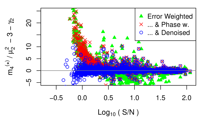
(d)
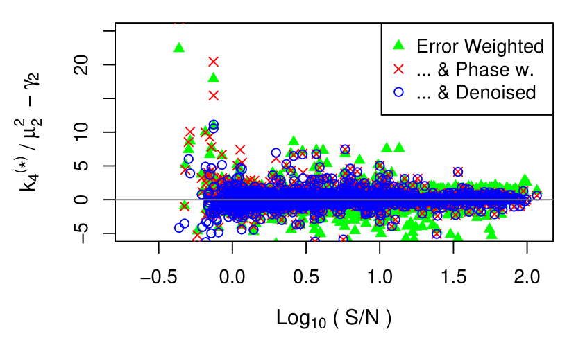
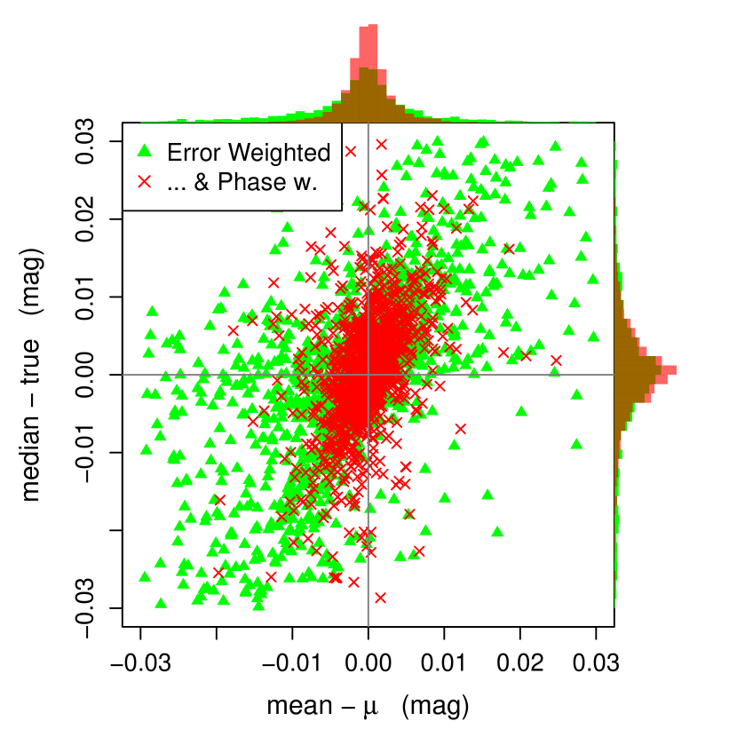
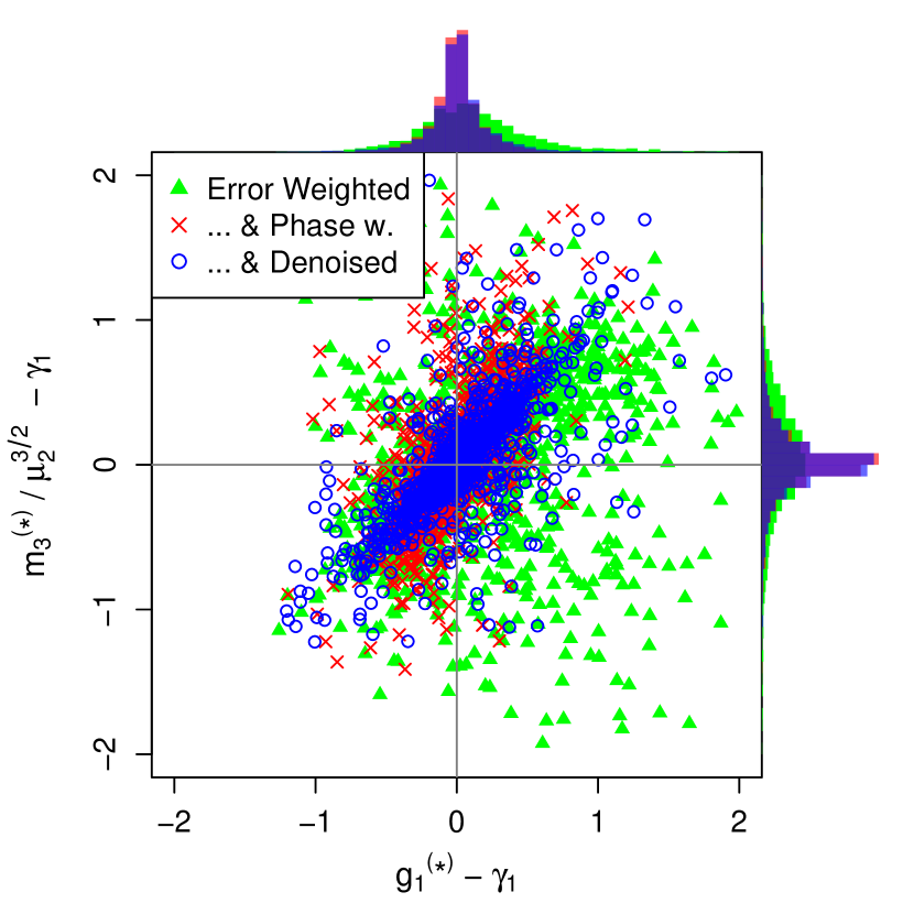
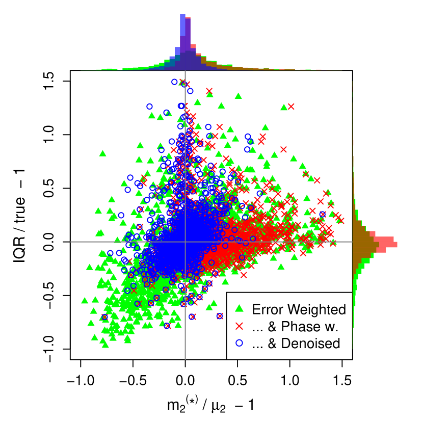
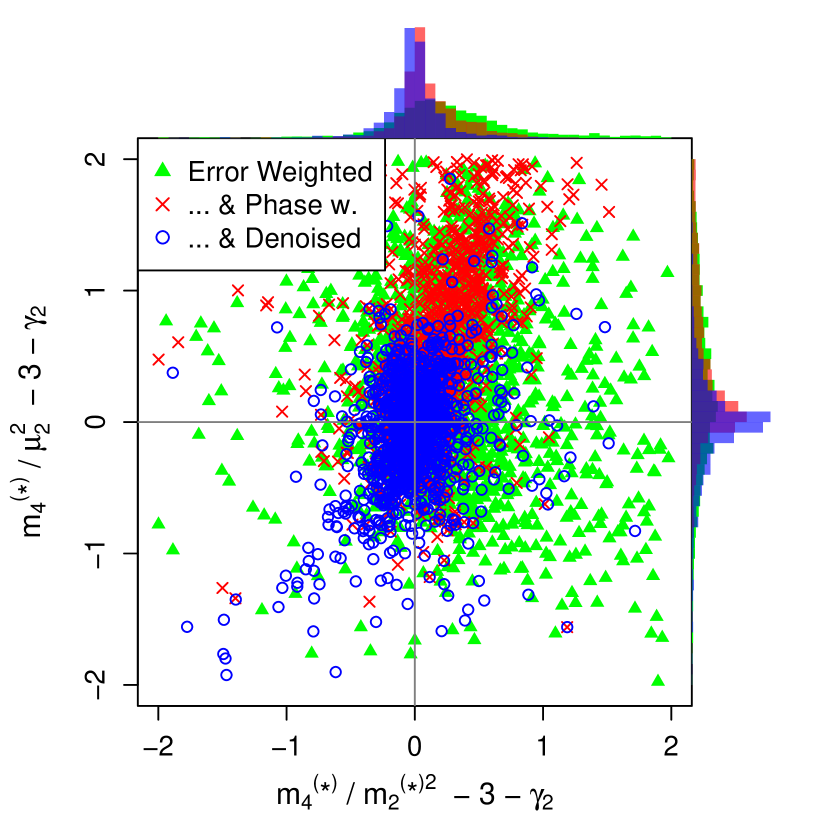
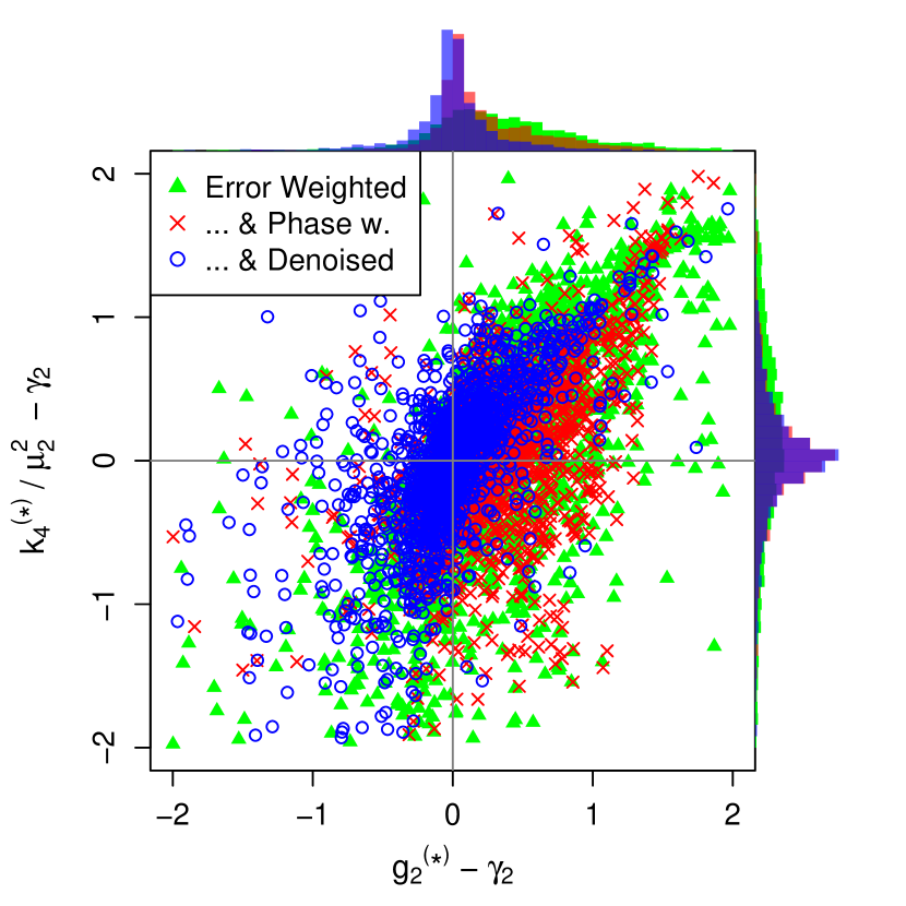
Estimators which provide similar information (such as the mean and median, variance and interquartile range, skewness and kurtosis standardized by the estimated or true variance) are compared in scatter plots in Appendix D. Although contributions from different ratios are not distinguished, error-phase weighted (and noise-unbiased, when applicable) estimators are always associated with more strongly peaked distributions around the true values than the error-weighted analogues.
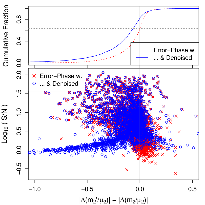
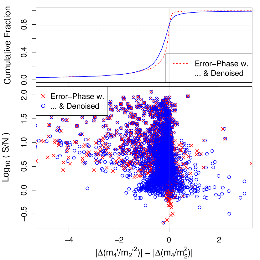
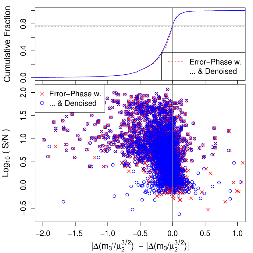
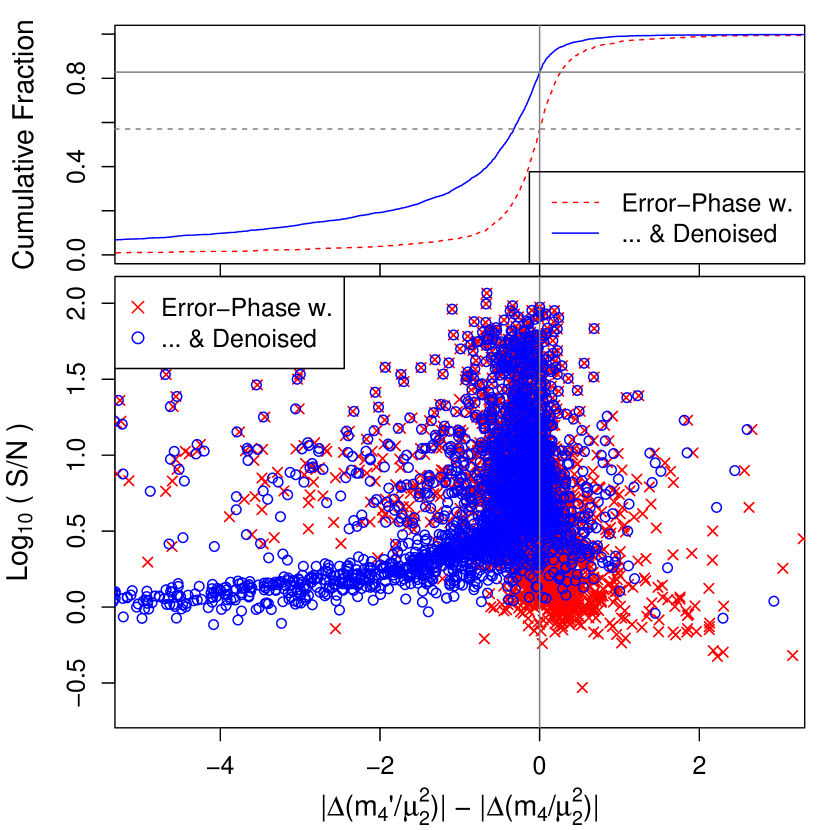
In order to quantify the effect of error-phase weighting and additional denoising with respect to simple error weighting, the top panels in Figs 4–6 indicate the fraction of sources associated with estimators improved by phase weights and noise correction. The accuracy of a generic estimator is assessed by its distance from the true value . The abscissas in Figs 4–6 represent the difference between the distance of error-phase weighted (and noise-unbiased, when applicable) estimators and the one of error-weighted estimators from the correct values: negative differences indicate smaller distances to the true values and thus improved accuracy with respect to error-weighted estimators. The accuracy of error-phase weighted and noise-unbiased estimators improved in 70-to-90 per cent of the cases and deteriorations were typically smaller in frequency and magnitude than improvements. In the singular case of the standardized skewness , denoising worsened almost 8 per cent of the estimates with respect to error-phase weighting. As apparent in Fig. 5a, the accuracy of the standardized noise-unbiased skewness worsened at low ratios. This was expected because the noise-unbiased variance might be easily underestimated when uncertainties are of the same order as the signal, and the normalization of the skewness by a much smaller number than the correct one could rapidly degrade the precision of the estimator. A similar (less pronounced) tendency at low ratios was also observed in the case of the standardized kurtosis.
(a)

(c)
(b)

(d)

(a)
(c)
(b)
(d)
(a)

(b)
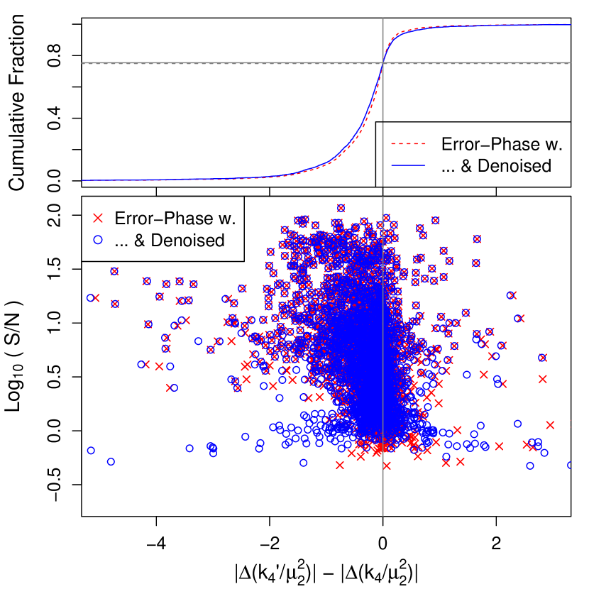
As noted in Rimoldini (2013b), the noise-unbiased variance can become too small at low levels, overestimating the standardized noise-unbiased skewness and kurtosis, or leading to an undetermined skewness value in case of non-positive variance. On the other hand, when the variance is not corrected by noise biases, it is generally overestimated, and if the true values of skewness or kurtosis are sufficiently close to zero, the standardized noise-biased skewness and kurtosis become more accurate (by serendipity).
4.2 Automated classification
The effect of statistical parameters weighted by different schemes on automated classification was assessed by comparing the classification accuracy and precision as a function of variability type employing unweighted, error-weighted, phase-error weighted and noise-unbiased phase-error weighted estimators.
4.2.1 Attributes and variability types
Automated classification of stellar variability types was pursued with a set of attributes which characterized features of different classes. Some studies employed only information from light-curve modelling (Debosscher et al., 2007, 2009; Blomme et al., 2010, 2011), with additional statistical parameters (Richards et al., 2011) or colour information (Sarro et al., 2009), while attributes from modelling, statistical and astrophysical quantities were used in Dubath et al. (2011); Rimoldini et al. (2012).
The list of attributes employed for classification herein was restricted to descriptive statistics (mean, median, variance, interquartile range, normalized and non-normalized skewness and kurtosis), in order to test the effect of different weighting schemes on classification. Only variability types which could be identified by the distribution of measurements were included in the training set, such as eclipsing binaries, RR Lyrae, Mira, Cephei and Alpha2 Canum Venaticorum stars, accounting for over 60 per cent of all sources in the Hipparcos periodic catalogue.
In these classification experiments, statistical parameters did not depend on modelling and were computed on the original (not simulated) data, which thus included the sources previously excluded because of modelling issues. The same quality flags, periods and weighting schemes were applied as described in Sec. 4.1. Since the true signal variance was unknown, the ratio was estimated by substituting the unknown in Eq. (20) with the noise-unbiased phase-weighted sample variance and by weighting the average of squared errors in the denominator with the same weights for consistency:
| (21) |
The ratios of the sources selected for classification (as described in Sec. 4.2.2) spanned a range from 0.4 to 140.
4.2.2 Data selection
Sources from the Hipparcos periodic catalogue were cross-matched with classifications from literature as available in the Variable Star Index (Watson, Henden & Price, 2012)111111See http://www.aavso.org/vsx/index.php?view=about.top for more details on how literature information has been selected, maintained and revised. A comprehensive list of variability types, labels and their descriptions is available at http://www. aavso.org/vsx/help/VariableStarTypeDesignationsInVSX.pdf of the American Association of Variable Star Observers (AAVSO) with the nearest object within 1 arcsec.121212Only one source, Hip 31400, was not considered because associated with different classes at very similar angles from the direction of the Hipparcos source.
Uncertain classifications (with class labels followed by the mark ‘:’) were excluded, unless the uncertainty referred to properties of eclipsing binaries other than light-curve shapes, such as the physical characteristics, the luminosity class of the components, or the degree of filling of the inner Roche lobes. Objects associated with combinations of different classes (with labels joined by the symbol ‘+’) were not addressed herein. The subset of variability types chosen to test classification with statistical parameters are listed in Table 1 and include 1605 sources associated with class labels EA, EB, EW, ACV, M, RRAB, RRC, DCEP and DCEPS, defined in Table 1 together with the corresponding sample sizes. Sources which poorly represented their class were not removed from the training set in order to avoid the introduction of selection biases (e.g., by favouring objects with higher ratios) and because the focus of this application was related to the relative classification accuracy employing attributes with different weighting schemes.
| Variability Type | Label | Number |
|---|---|---|
| Eclipsing Binary: Algol type | EA | 409 |
| Beta Lyrae type | EB | 208 |
| W Ursae Majoris type | EW | 170 |
| Alpha2 Canum Venaticorum | ACV | 183 |
| Mira Ceti | M | 218 |
| RR Lyrae: Asymmetric light curve | RRAB | 139 |
| Nearly symmetric light curve | RRC | 28 |
| Delta Cephei | DCEP | 220 |
| First overtone pulsators | DCEPS | 30 |
| Total: | 1605 |
4.2.3 Training-set attributes
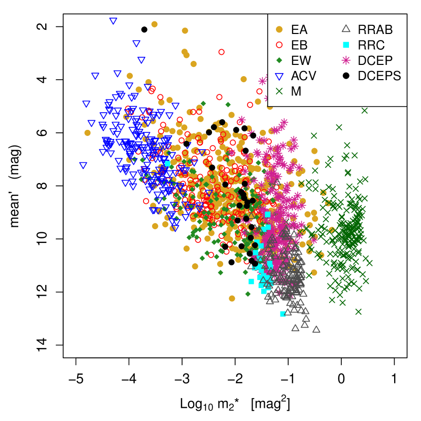
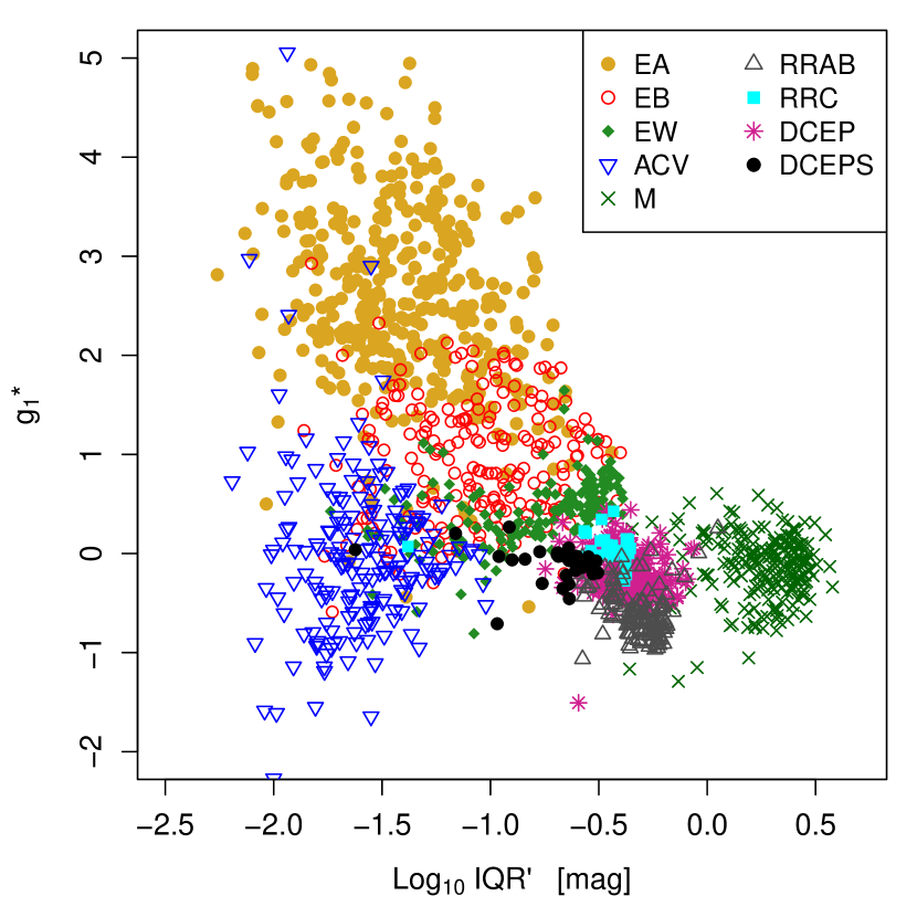
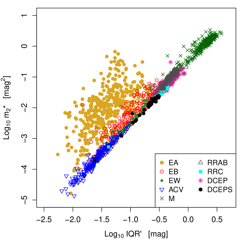
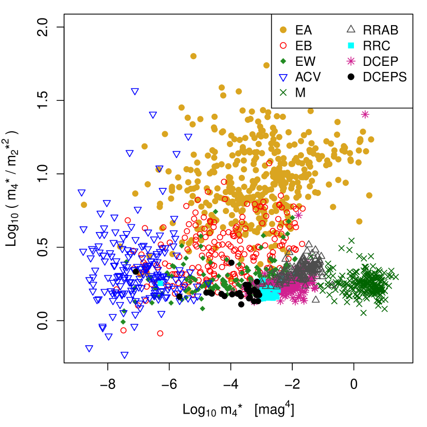
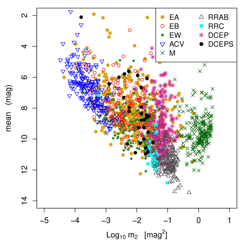
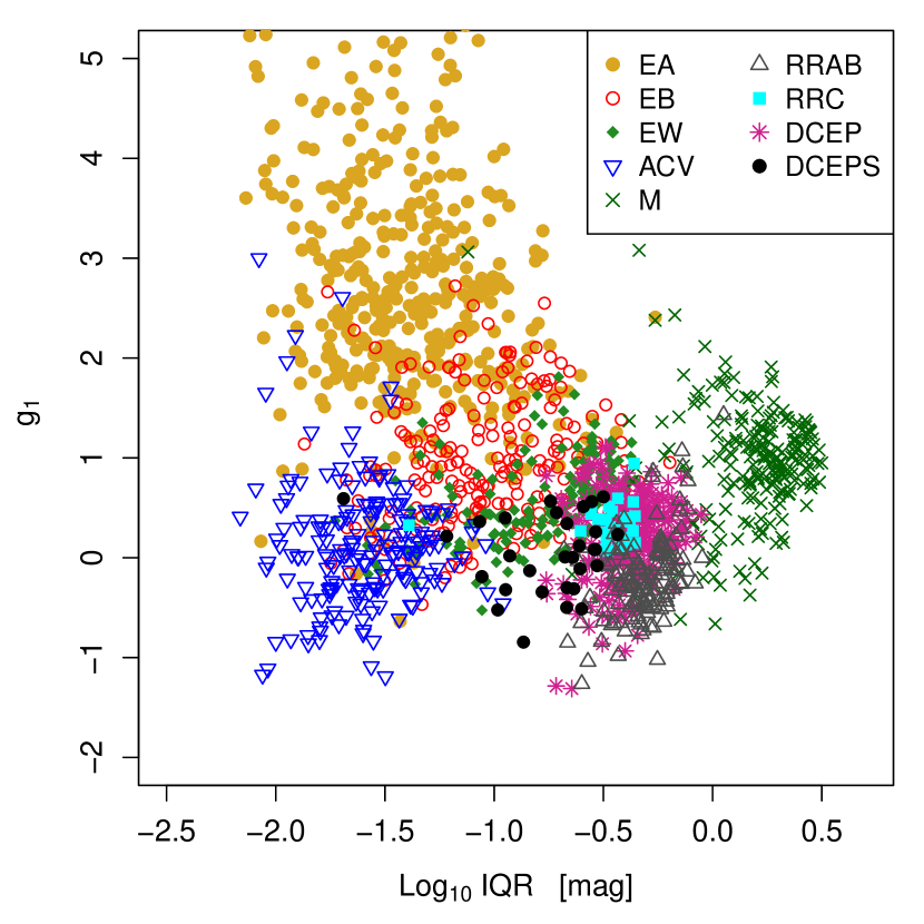
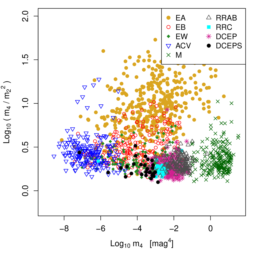
The distributions of a selection of error-phase weighted (and noise-unbiased, when applicable) statistical parameters as a function of variability type are presented in Fig. 7. The mean or median magnitudes of sources at broadly different distances from the observer do not provide information on the intrinsic source properties. However, the correlation between magnitude and noise, coupled with the interquartile range or variance (as shown in Fig. 7a), is related to the level and thus to an observational selection. Figure 7b illustrates clearly the difference between robust and non-robust estimators for the same quantity, such as the interquartile range versus the variance, which proves effective at separating eclipsing binaries (mostly EA and some fraction of EB types). The interquartile range and standardized skewness are presented in Fig. 7c: the skewness separates the eclipsing binary subtypes from most other classes, which are better distinguished by the interquartile range. A similar scatter plot is shown in Fig. 7d in terms of normalized and non-normalized kurtosis moments, with the difference that some classes occupy different relative loci (such as the EA types and the RRAB with respect to DCEP variables).
The estimators and variability types illustrated in Fig. 7 are also presented for the unweighted case in Appendix E. The distributions of most unweighted estimators in Fig. 14 tend to be more scattered than the ones shown in Fig. 7. In the case of ACV stars, instead, the unweighted skewness and kurtosis are less scattered, because these sources have very low ratios (typically ) and the correction of noise biases at such levels can decrease significantly the precision of higher moments (Rimoldini, 2013b). Another noticeable difference between Figs 7 and 14 is related to the larger skewness of Mira stars in the unweighted case, which can be understood by the systematic difference in the uncertainties associated with faint and bright measurements (e.g., van Leeuwen, 1997). Such a difference is enhanced by the large amplitudes of light variations of Mira types, so that greater uncertainties on the faint side of the signal generate more faint than bright ‘outliers’, biasing the unweighted skewness towards greater values.
(a)
(c)
(b)
(d)
4.2.4 Classification method
Automated classification tests were performed employing random forests (Breiman, 2001).131313This work employed the randomForest package implemented in R (R Development Core Team, 2013) by Liaw & Wiener (2002). Random forest is an accurate tree-based classification method (e.g., see Richards et al., 2011), quite robust to outliers and strongly correlated attributes. The accuracy of the classifier was estimated from a subset of sources (about one-third of all objects) randomly omitted from the learning process and thus called ‘out-of-bag’ sources. The importance of an attribute for classification was measured by the mean decrease in accuracy after permuting the values of that attribute in the out-of-bag sources (see Rimoldini et al., 2012, for more details).
The random forest classifier was trained with estimators employing a single weighting scheme per run, i.e., unweighted, error-weighted, error-phase weighted or noise-unbiased error-phase weighted. For each weighting scheme, random forest was executed 1000 times with 500 trees and the classification accuracy and precision rates were aggregated after each run in order to assess their mean and dispersion.
4.2.5 Results
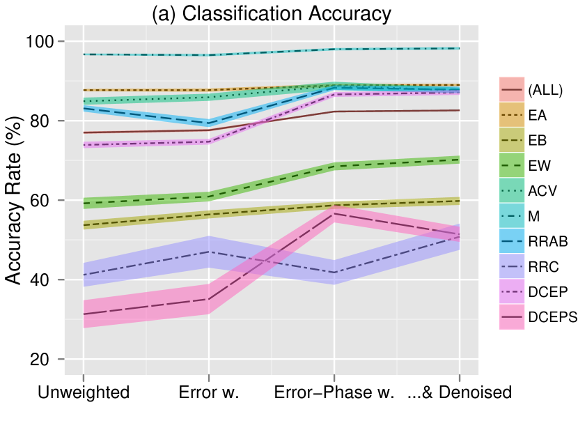
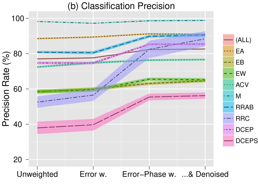
The mean classification accuracy and precision rates are listed as a function of variability type and attribute weighting scheme in Tables 2 and 3, and illustrated in Figs 8a and 8b, respectively. Training-set sources were reclassified by sole statistical parameters with an overall accuracy from 77.0 to 82.6 per cent on average, depending on the weighting scheme adopted. Unweighted estimators led to the smallest accuracy level, closely followed by error-weighted estimators at 77.6 per cent. The introduction of phase weights improved the accuracy to 82.3 per cent and noise-unbiased error-phase weighted estimators achieved the best overall classification accuracy of 82.6 per cent (with uncertainty at the level of 0.2 to 0.3 per cent). The overall trends were generally reflected by single variability types with only a few exceptions. In particular, error-weighted estimators of RRAB types led to significantly worse classification accuracy than unweighted estimators. This was explained by the relatively large amplitude of RRAB variables, which enhanced the systematic difference of uncertainties between bright and faint measurements in the light curve: weighting by errors decreased the importance of faint measurements, increasing the similarity (and thus confusion) with DCEP and M-type light curves. In the case of DCEPS variables, denoising was marginally counterproductive for accuracy, although still significantly better with respect to the unweighted or error-weighted schemes. This was expected to be related to the increased confusion with the noise-unbiased estimators of EW types, which were more numerous and extended to lower ratios than the DCEPS stars: while the distributions of the standardized error-phase weighted kurtosis moments of DCEPS and EW types could just be separated, the additional denoising decreased the values of standardized kurtosis moments more for the EW than the DCEPS stars, leading to overlapping distributions dominated by the EW types.
| Var. | Error | Error-Phase | Err.-Ph. w. | |
|---|---|---|---|---|
| Type | Unweighted | Weighted | Weighted | & Denoised |
| EA | 87.7 0.3 | 87.7 0.4 | 88.9 0.4 | 89.0 0.3 |
| EB | 53.7 1.1 | 56.4 1.0 | 58.7 0.9 | 59.8 1.0 |
| EW | 59.2 1.4 | 60.9 1.2 | 68.5 1.0 | 70.2 1.0 |
| ACV | 84.9 0.9 | 85.9 0.9 | 88.8 1.0 | 87.6 0.7 |
| M | 96.7 0.2 | 96.5 0.3 | 98.0 0.3 | 98.2 0.3 |
| RRAB | 83.1 0.8 | 79.4 1.0 | 88.3 0.6 | 87.8 0.8 |
| RRC | 41.2 3.0 | 47.0 4.0 | 41.8 3.1 | 50.8 3.3 |
| DCEP | 73.9 0.8 | 74.7 0.7 | 86.6 0.6 | 87.1 0.6 |
| DCEPS | 31.3 3.5 | 35.1 3.8 | 56.6 2.2 | 51.4 1.9 |
| ALL | 77.0 0.3 | 77.6 0.3 | 82.3 0.2 | 82.6 0.2 |
Precision rates of classification per variability type showed successive improvements (consistent within uncertainties) from the unweighted to the error-weighted, error-phase weighted and noise-unbiased schemes. A single exception was related to Mira stars: their classification precision with error-weighted estimators was about one per cent worse than with unweighted attributes, as a consequence of the increased contamination by RRAB stars (as explained above).
| Var. | Error | Error-Phase | Err.-Ph. w. | |
|---|---|---|---|---|
| Type | Unweighted | Weighted | Weighted | & Denoised |
| EA | 88.5 0.4 | 89.4 0.4 | 91.2 0.4 | 91.0 0.3 |
| EB | 58.4 1.0 | 59.9 1.0 | 63.1 0.9 | 64.5 0.8 |
| EW | 58.5 1.1 | 59.4 1.0 | 65.5 0.9 | 65.2 0.9 |
| ACV | 72.4 0.5 | 74.8 0.6 | 76.3 0.5 | 76.6 0.5 |
| M | 98.2 0.2 | 97.2 0.2 | 98.6 0.3 | 98.8 0.3 |
| RRAB | 80.8 0.7 | 80.5 0.9 | 89.8 0.8 | 90.5 0.9 |
| RRC | 52.5 3.2 | 56.5 3.3 | 82.4 4.9 | 88.4 4.3 |
| DCEP | 74.7 0.8 | 74.7 0.8 | 85.3 0.6 | 85.4 0.6 |
| DCEPS | 37.9 3.5 | 39.7 3.3 | 55.4 1.9 | 56.2 1.8 |
| ALL | 77.0 0.3 | 77.6 0.3 | 82.3 0.2 | 82.6 0.2 |
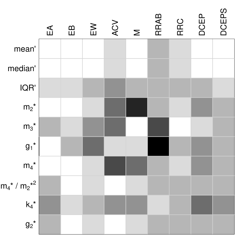
The importance of phase-weighted (and noise-unbiased, when applicable) attributes as a function of variability type from a run of random forest is depicted in Fig. 9, with darker cells indicating more important attributes for a given class. For example, the skewness confirmed to be particularly useful to distinguish eclipsing binaries and the asymmetric light curves of RRAB stars. Also, large and small amplitude variables, such as ACV and M types, could easily be separated by the variance.
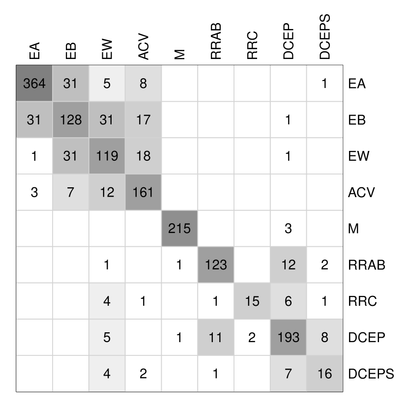
The confusion matrix from a run of random forest, employing error-phase weighted (and noise-unbiased, when applicable) estimators, is shown in Fig. 10. The overall classification accuracy was 83 per cent and reached 92 per cent after aggregating the subtypes of eclipsing binary, RR Lyrae and Delta Cephei into their superclasses. The improvement in classification accuracy, with respect to results employing unweighted estimators, was about 6 per cent in both cases of separated and aggregated variability subtypes. The level of confusion between eclipsing binaries of EA, EB and EW types was expected from the natural overlap in their definitions. The misclassification of many ACV types as eclipsing binaries was attributed to the restricted set of attributes employed herein (e.g., the attribute ‘QSO variations’ in Rimoldini et al., 2012, proved to be useful in this context). Similarly, the confusion between RR Lyrae and Delta Cephei variables would not have occurred if the period was included in the set of classification attributes. On the other hand, simple amplitude estimators such as variance and interquartile range were sufficient to separate Mira stars from most other classes with high accuracy (as apparent in Fig. 7).
5 Conclusions
A simple weighting scheme based on linear interpolation, applicable in phase or time, was proposed in order to improve the accuracy of descriptive statistics of unevenly sampled time series. Weights represented by time intervals could be applied to well-sampled deterministic signals. For sparsely sampled but periodic time series (dominated by a single period), light curves could be folded with the fundamental periods and weights expressed in terms of phase intervals.
The Hipparcos catalogue of periodic variables represented a suitable test bed of unevenly sampled light curves with realistic distributions of variability types to investigate the accuracy of estimators weighted by different schemes. Noise-unbiased estimators weighted by phase intervals (or inverse-squared uncertainties at low ratios) improved the accuracy for 70-to-90 per cent of the sources with respect to the values of the error-weighted counterparts. Deteriorations in accuracy were observed in 10-to-30 per cent of the cases, with magnitudes typically smaller than the ones corresponding to improvements.
Automated classification experiments confirmed that the best overall results were achieved employing the set of the most accurate attributes, i.e., the noise-unbiased estimators weighted by phase intervals and inverse-squared uncertainties at high and low ratios, respectively. The overall improvement in classification accuracy with respect to the result employing unweighted estimators was about 6 per cent and most of it was related to the introduction of phase weights which adapted to the varying sampling density of the light curve.
Acknowledgments
The author is grateful to M. Süveges, P. Dubath and the anonymous referee for useful comments on the original manuscript. This work made use of the Hipparcos catalogue obtained from the European Space Agency astrometric mission Hipparcos, the VizieR service, operated at the Centre de Données astronomiques de Strasbourg (Strasbourg, France) and the International Variable Star indeX (VSX), operated by the American Association of Variable Star Observers (Cambridge, Massachusetts, USA).
References
- Auvergne et al. (2009) Auvergne M. et al., 2009, A&A, 506, 411
- Blomme et al. (2010) Blomme J. et al., 2010, ApJ, 713, L204
- Blomme et al. (2011) Blomme J. et al., 2011, MNRAS, 418, 96
- Borucki et al. (2010) Borucki W.J. et al., 2010, Science, 327, 977
- Breiman (2001) Breiman L., 2001, Machine Learning, 45, 5
- Carbonell, Oliver & Ballester (1992) Carbonell M., Oliver R., Ballester J.L., 1992, A&A, 264, 350
- Debosscher et al. (2007) Debosscher J., Sarro L.M., Aerts C., Cuypers J., Vandenbussche B., Garrido R., Solano E., 2007, A&A, 475, 1159
- Debosscher et al. (2009) Debosscher J. et al., 2009, A&A, 506, 519
- Dubath et al. (2011) Dubath P. et al., 2011, MNRAS, 414, 2602
- ESA (1997) European Space Agency, 1997, The Hipparcos and Tycho Catalogues, ESA SP-1200
- Eyer (1998) Eyer L., 1998, Les étoiles variables de la mission HIPPARCOS, PhD Thesis No 3002, Université de Genève
- Eyer & Mignard (2005) Eyer L., Mignard F., 2005, MNRAS, 361, 1136
- Eyer et al. (1994) Eyer L., Grenon M., Falin J.-L., Froeschle M., Mignard F., 1994, Solar Physics, 152, 91
- Ivezić et al. (1994) Ivezić Ž. et al., 2011, preprint (arXiv:0805.2366)
- Kaiser et al. (2002) Kaiser N. et al., 2002, in Tyson J. A., Wolff S., eds, Proc. SPIE Vol. 4836, Survey and Other Telescope Technologies and Discoveries. SPIE, Bellingham, p. 154
- Koen (2005) Koen C., 2005, MNRAS, 361, 887
- Liaw & Wiener (2002) Liaw A., Wiener M., 2002, R News, 2 (3), 18
- Perryman et al. (1997) Perryman M.A.C. et al., 1997, A&A, 323, L49
- Perryman et al. (2001) Perryman M.A.C. et al., 2001, A&A, 369, 339
- R Development Core Team (2013) R Development Core Team, 2013, R: A Language and Environment for Statistical Computing, R Foundation for Statistical Computing, Vienna, Austria
- Richards et al. (2011) Richards J.W. et al., 2011, ApJ, 733, 10
- Rimoldini et al. (2012) Rimoldini L. et al., 2012, MNRAS, 427, 2917
- Rimoldini (2013a) Rimoldini L., 2013a, preprint (arXiv:1304.6564)
- Rimoldini (2013b) Rimoldini L., 2013b, preprint (arXiv:1304.6715)
- Rybicki & Press (1992) Rybicki G.B., Press W.H., 1992, ApJ, 398, 169
- Ruppert, Wand, & Carroll (2003) Ruppert D., Wand M.P., Carroll R.J., 2003, Nonparametric Regression, Cambridge University Press
- Sarro et al. (2009) Sarro L.M., Debosscher J., Aerts C., López M., 2009, A&A, 506, 535
- Scargle (1989) Scargle J.D., 1989, ApJ, 343, 874
- Scargle (1990) Scargle J.D., 1990, ApJ, 359, 469
- Stuart & Ord (1969) Stuart A., Ord J., 1969, Kendall’s Advanced Theory of Statistics, Charles Griffin & Co. Ltd, London
- van Leeuwen (1997) van Leeuwen F., 1997, Sp. Sci. Rev., 81, 201
- Vio, Strohmer & Wamsteker (2000) Vio R., Strohmer T., Wamsteker W., 2000, PASP, 112, 74
- Watson et al. (2012) Watson C., Henden A.A., Price A., 2012, VizieR Online Data Catalogue, AAVSO International Variable Star Index, Version 2012-09-23
Appendix A Periodic interpolation
Substituting time-sorted data with phase-sorted measurements in Eq. (2) and adding the interpolation term from the last to the first point in phase, it follows:
| (22) | ||||
| (23) | ||||
| (24) | ||||
| (25) |
where and , so that
| (26) | |||
| (27) | |||
| (28) |
and
| (29) |
When differences between successive phases are a significant fraction of a cycle, they might be limited to some maximum interval as follows:
| (30) | ||||
| (31) | ||||
| (32) |
and, of course, then .
Appendix B The Hipparcos periodic light curves
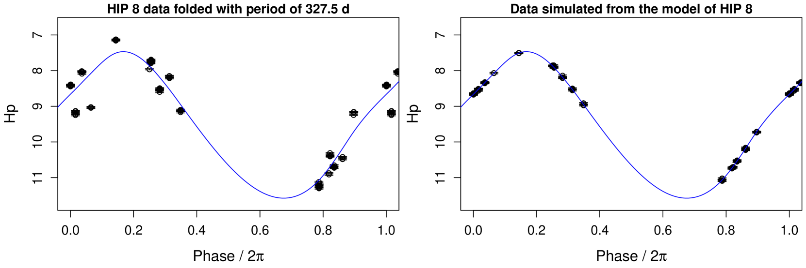
Light curves of the Hipparcos periodic variables are illustrated in Fig. 11. Panels on the left-hand side show the Hipparcos data folded with the catalogue period, while the right-hand panels present data simulated around the model according to the measurement uncertainties (assumed Gaussian) and the observed phases. Simulated data were employed to assess the accuracy of statistical estimators (with respect to the model), while classification was performed on the original data. Figure 11 provides sample light curves for 4 of the 2683 Hipparcos sources available online (see supporting information).141414The 29 objects with no data associated with good quality flags (i.e., field HT4 only) were not included in Fig. 11.
Appendix C Statistical parameters
The statistical estimators employed to test different weighting schemes are defined below.
C.1 Variance, skewness and kurtosis
Sample noise-unbiased weighted moments and cumulants are defined following Rimoldini (2013b). Denoting the sample weighted central moments of order by
| (33) |
and representing the Gaussian uncertainties by , the noise-unbiased estimators (starred) are defined as follows:
| (34) | ||||
| (35) | ||||
| (36) | ||||
| (37) | ||||
| (38) | ||||
| (39) | ||||
| (40) |
C.2 Percentiles
Percentiles depend on the rank of sorted values, thus they are less sensitive to extreme values than moments and cumulants which involve powers of deviations from the mean and average over all elements. The -th percentile is defined as the (interpolated) value such that per cent of the data are smaller than . Two common percentiles are the median and interquartile range .
Denoting the list of measurements sorted in increasing values by , associated with weights , respectively, the -th weighted percentile is defined as follows:
| (41) |
where
| (42) |
Appendix D Scatter plots of related estimators
Figures 12–13 compare statistical parameters which provide similar information, such as robust versus non-robust or normalized versus non-normalized estimators, as a function of the weighting scheme. Error-phase weighted (and noise-unbiased, when applicable) estimators correspond to the most strongly peaked distributions around the correct values.
(a)
(c)
(b)
(d)
Appendix E Unweighted estimators as a function of variability type
Figure 14 presents a selection of unweighted estimators for stars of different variability types. This Figure is intended to be compared to Fig. 7, which illustrates the same information for phase-error weighted and noise-unbiased estimators.
(a)
(c)
(b)
(d)
Supporting Information
Additional Supporting Information may be found in the online version of this paper:
Figure B1. The folded light curves from the Hipparcos periodic catalogue and the smoothing spline models employed to generate simulated data.