Robust error correction for real-valued signals via message-passing decoding and spatial coupling

Abstract

We revisit the error correction scheme of real-valued signals when the codeword is corrupted by gross errors on a fraction of entries and a small noise on all the entries. Combining the recent developments of approximate message passing and the spatially-coupled measurement matrix in compressed sensing we show that the error correction and its robustness towards noise can be enhanced considerably. We discuss the performance in the large signal limit using previous results on state evolution, as well as for finite size signals through numerical simulations. Even for relatively small sizes, the approach proposed here outperforms convex-relaxation-based decoders.

I Introduction

Although information is discrete in the classical coding theory, there are situations of interest where one should consider real-valued signals, such as scrambling of discrete time analog signals for privacy [1], network [2, 3] or jointed source and channel coding [4], or in the impulse noise cancellation in orthogonal frequency division multiplexing system [5]. To perform error correction for such real signals over a channel with a gross errors on a fraction of elements (and small noise for all of them) a compressed-sensing-based scheme has been proposed by Donoho and Huo [6] and Candes and Tao [7]. Here we reconsider this problem, taking full advantage of the recent progresses in compressed sensing theory.

The problem is easily stated. One is given a real-valued signal x, and a channel that adds gross errors to a fraction of elements. Is there a way to encode the signal such that the errors added by the channel can be corrected? Can this approach still be used when the channel is in addition adding a small noise to all elements (a situation arguably much closer to some real channels [6, 8, 9])? The method proposed in [6, 7, 8] is to first multiply the signal x by a random matrix in order to create a codeword of larger dimension, and then to use the classical compressed sensing approach, based on convex-relaxation decoding, to correct the errors of transmission.

Our contribution in the present paper is three-fold. (1) We replace the convex-relaxation decoding by the Bayesian Approximate Message-Passing (AMP) decoder that uses the available prior information about the error vector [10, 11]. This provides a significant improvement in performances. (2) We consider a quasi-sparse channel where, in addition to the gross errors on a fraction of elements, there is a small additive random white noise, and in the lines of [12] show that the performance of AMP decoder is stable under this additional noise. (3) We use spatially-coupled measurement matrices in the decoding [11, 13], which allows to further enhance the possibility for error correction (and up to its information-theoretical limit in the case of strictly sparse noise).

Our paper relies on the development of the Bayesian AMP algorithm [10, 11, 14, 15], whose behavior for large signal sizes can be studied rigorously using the state evolution technique [16, 17]; on the development of spatially coupled error correcting codes on binary variables, see [18] for a review, and related measurement matrices in compressed sensing [11, 13, 19]; and on the use of quasi-sparsity in the Bayesian approach [12]. While the analysis of the reconstruction performance of AMP are rigorous in the large signal limit, we also consider the performance for finite size signals through numerical experiments.

II Compressed-sensing Based Error-Correction

Consider a real-valued vector of information ${\textbf{x}}\!\in\!\mathbb{R}^{N}$, encode this vector by a full-rank real $M\!\times\!N$ matrix $A$, with $R\!=\!N/M\!<\!1$ being the coding rate (the redundancy rate introduced in the code), so that the encoded vector is ${\textbf{y}}=A{\textbf{x}}\in\mathbb{R}^{M}$. Since $A$ is full rank, one can recover the original signal x from the encoded one multiplying by the pseudo-inverse. The encoded signal is sent through a noisy channel and gives rise to the corrupted codeword ${\tilde{\textbf{y}}}={\textbf{y}}+{\textbf{e}}$ where the element of e are iid with a distribution

$$P(e_{i})=\rho{\cal N}(0,1+\epsilon)+(1-\rho){\cal N}(0,\epsilon)\,,$$ (1)

where $0<\rho<1$. We thus have a fraction $\rho$ of elements with gross (variance $1+\epsilon$) errors, the rest having small (variance $\epsilon$) amplitudes. One then considers a full rank ”parity-check”-like matrix $F$ such that $FA=0$. We construct such a pair of matrices by first choosing a $P\times M$ matrix $F$ with independent normally distributed elements of zero mean and variance $1/M$ (or variance specified by the seeding matrix, see later), the kernel of $F$ is then the range of the encoding matrix $A$ . One must have $P\leq M-N$, in order to maximize the coding rate $R=N/M$, we take from now on $P=M-N$. The application of $F$ to the corrupted signal ${\tilde{\textbf{y}}}$ results in the real-valued vector

$${\textbf{h}}=F({\textbf{y}}+{\textbf{e}})=F{\textbf{e}}\,,$$ (2)

where h has dimension $M-N$ and e is a quasi-sparse vector of dimension $M$. This is a compressed sensing problem: reconstruct the quasi-sparse $M$-dimensional error e given $M-N$ of its linear projections (measurements) h. In the context of compressed sensing $F$ is the measurement matrix.

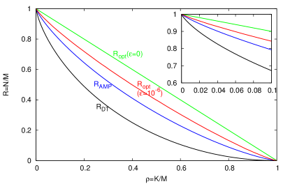
Let us first review the possibility of this error-correction scheme when the error e is exactly sparse, i.e. $\epsilon=0$. Using an intractable $\ell_{0}$ minimization, the gross error e in eq. (2) can be found exactly as long as $M-N>M\rho$. So error correction in real valued signals corrupted by sparse gross noise is possible (but may be hard) for coding rates $R<R_{\rm opt}=1-\rho$. Popular tractable $\ell_{1}$ minimization, as used in [7, 8], recovers the error e exactly when $M-N\geq\alpha_{\rm DT}M$, where $\alpha_{\rm DT}$ is the Donoho-Tanner measurement rate [20]. This means that the coding rate must be lower than $R\leq R_{\rm DT}=1-\alpha_{\rm DT}$. These two transitions are depicted in Fig. 1 and one can see that $R_{\rm DT}$ is considerably lower than $R_{\rm opt}$. A first step to improvement is to decode with an approximate message passing approach.

Figure 1: Phase diagram showing the coding rate $R=N/M$ below which error correction can be performed over a channel with noise described by eq. (1), plotted as a function of the noise sparsity $\rho$, zoom in the inset. The black (bottom) curve $R_{\rm DT}$ depicts the limit of performance of the $\ell_{1}$-minimization approach for $\epsilon=0$. The blue (2nd from bottom) curve shows the limit of performance of the Bayesian AMP approach for $\epsilon=0$, note that up to about $\epsilon\lesssim 10^{-5}$ this curve does not change visibly. The green (top) curve, given by $R_{\rm opt}=1-\rho$, depicts the highest possible coding rate for which exact decoding is possible for $\epsilon=0$. Below the red (2nd from top) line error correction with MSE comparable to $\epsilon=10^{-6}$ is possible with the Bayes optimal estimation of the error vector. These two rates $R_{\rm opt}$ can be reached in the limit of large signal size using the seeded Bayesian AMP approach.

III Decoding with approximate message passing

Consider the compressed sensing problem in eq. (2) to reconstruct the vector e based on the knowledge of the $M-N$-dimensional h and the matrix $F$. When the distribution of the error elements is known, the Bayes optimal way of estimating $\hat{\textbf{e}}$ that minimizes the MSE $E=\sum_{i=1}^{M}(e_{i}-\hat{e}_{i})^{2}/M$ with the true error e is given as

$$\hat{e}_{i}=\int\text{d}e_{i}\,e_{i}\,\nu_{i}(e_{i})\,,$$ (3)

where $\nu_{i}(e_{i})$ is the marginal probability distribution of the variable $i$

$$\nu_{i}(e_{i})\equiv\int_{\{e_{j}\}_{j\neq i}}P({\textbf{e}}|{\textbf{h}})\prod_{j\neq i}de_{j}$$ (4)

under the posterior measure

$$P({\textbf{e}}|{\textbf{h}})=\frac{1}{Z({\textbf{h}})}P({\textbf{e}})\prod_{\mu=1}^{M-N}\delta(h_{\mu}-\sum_{i=1}^{M}F_{\mu i}e_{i})\,.$$ (5)

Such an optimal Bayes reconstruction is not computationally tractable in general and in order to get an estimate of the marginals $\nu_{i}(e_{i})$, we use the AMP algorithm.

III-A AMP reminder

AMP is defined over a graphical model and iteratively updates pre-estimates of the mean and variance $R_{i}$, $\Sigma_{i}^{2}$ and a posteriori estimates of the mean and variance $a_{i}$, $v_{i}$ for each component $i$ of $\hat{\textbf{e}}$. They are updated as follows (for the derivation in the present notation see [15] and for the original one [14, 10]) where, for convenience, we have also defined for every component $\mu$ of h auxiliary variables $V_{\mu}$ and $\omega_{\mu}$:

$$V^{t+1}_{\mu} = \sum_{i}F_{\mu i}^{2}\,v^{t}_{i}\,,$$ (6)

$$\omega^{t+1}_{\mu} = \sum_{i}F_{\mu i}\,a^{t}_{i}-\frac{(h_{\mu}-\omega^{t}_{\mu})}{V^{t}_{\mu}}\sum_{i}F_{\mu i}^{2}\,v^{t}_{i}\,,$$ (7)

$$(\Sigma^{t+1}_{i})^{2} = \left[\sum_{\mu}\frac{F^{2}_{\mu i}}{V^{t+1}_{\mu}}\right]^{-1}\,,$$ (8)

$$R^{t+1}_{i} = a^{t}_{i}+\frac{\sum_{\mu}F_{\mu i}\frac{(h_{\mu}-\omega^{t+1}_{\mu})}{V^{t+1}_{\mu}}}{\sum_{\mu}\frac{F_{\mu i}^{2}}{V^{t+1}_{\mu}}}\,,$$ (9)

$$a^{t+1}_{i}\!\! = \!\!f_{a}\left((\Sigma^{t+1}_{i})^{2},R^{t+1}_{i}\right),v^{t+1}_{i}\!\!=\!\!f_{c}\left((\Sigma^{t+1}_{i})^{2},R^{t+1}_{i}\right)\,.$$

Where, using $P({\textbf{e}})=\prod_{i}P(e_{i})$ as given in eq. (1), the functions $f_{a}$ and $f_{c}$ read [12]

$$f_{a}(\Sigma^{2},R)=\frac{\sum_{a=1}^{2}w_{a}e^{-\frac{R^{2}}{2(\Sigma^{2}+\sigma_{a}^{2})}}\frac{R\sigma_{a}^{2}}{(\Sigma^{2}+\sigma_{a}^{2})^{\frac{3}{2}}}}{\sum_{a=1}^{2}w_{a}\frac{1}{\sqrt{\Sigma^{2}+\sigma_{a}^{2}}}e^{-\frac{R^{2}}{2(\Sigma^{2}+\sigma_{a}^{2})}}}\,,$$ (10)

$$f_{b}(\Sigma^{2},R)=\frac{\sum_{a=1}^{2}w_{a}e^{-\frac{R^{2}}{2(\Sigma^{2}+\sigma_{a}^{2})}}\frac{\sigma_{a}^{2}\Sigma^{2}(\Sigma^{2}+\sigma_{a}^{2})+R^{2}\sigma_{a}^{4}}{(\Sigma^{2}+\sigma_{a}^{2})^{\frac{5}{2}}}}{\sum_{a=1}^{2}w_{a}\frac{1}{\sqrt{\Sigma^{2}+\sigma_{a}^{2}}}e^{-\frac{R^{2}}{2(\Sigma^{2}+\sigma_{a}^{2})}}}\,,$$

$$f_{c}(\Sigma^{2},R)=f_{b}(\Sigma^{2},R)-f_{a}^{2}(\Sigma^{2},R)\,.$$ (11)

with

$$w_{1}=\rho\,,\quad\sigma_{1}^{2}=1+\epsilon\,,w_{2}=1-\rho\,,\quad\sigma_{2}^{2}=\epsilon\,.$$ (12)

The initialization is set as: $a_{i}^{t=0}=0$, $v_{i}^{t=0}=\rho+\epsilon$, $\omega_{\mu}^{t=0}=h_{\mu}$. Once the convergence of the iterative procedure is obtained the estimate of the $i$th component of the error $\hat{\textbf{e}}$ is $a^{t}_{i}$.

III-B Performance of AMP

As shown by Bayati and Montanari [16], in the limit of large system sizes, i.e. when parameters $\rho,\epsilon,R$ are fixed whereas $M\to\infty$, the evolution of the AMP algorithm can be described exactly using the “state evolution”. This allows to evaluate the MSE achieved by the AMP reconstruction. When $F$ is an homogeneous random iid matrix the state evolution is written in terms of MSE at iteration-time $t$, which evolves as (for a derivation see e.g. [14, 15, 16])

$$E^{t+1}\!=\!\!\sum_{a=1}^{2}w_{a}\int{\cal D}zf_{c}\left(\frac{1}{\hat{m}^{t}},z\sqrt{\sigma_{a}^{2}+\frac{1}{\hat{m}^{t}}}\right)\!\!,{\hat{m}}^{t}=\frac{\alpha}{E^{t}}\,,$$ (13)

where ${\cal D}z=dze^{-z^{2}/2}/\sqrt{2\pi}$ is a Gaussian measure for the integral, and where $E^{t=0}=\rho+\epsilon$.

The analysis of the Bayesian AMP for Gauss-Bernoulli noise e (that is, with $\epsilon=0$) has been considered in great details in [11, 15]. In that case AMP reconstructs perfectly the solution in a region larger than the $\ell_{1}$-minimization and up to the so-called spinodal transition $\alpha_{\rm AMP}$. In the notation of the present problem, where this leads exact decoding for considerably larger coding rates: The resulting $R_{\rm AMP}=1-\alpha_{\rm AMP}$ is shown in blue in Fig. 1 (with data adapted from [11]) where the advantage over the $\ell_{1}$-minimization decoding is clear. For a fraction of $\rho\!=\!0.1$ gross elements, for instance, the improvement goes from a necessary coding rate $R\approx 0.67$ for $\ell_{1}$ to $R\approx 0.79$ for AMP. It should be noted, however, that the $\ell_{1}$ performance is independent of the distribution of the gross error, whereas the Bayes AMP uses the distribution of the elements of the gross error. The properties of the channel are, however, often well known, in which case the improvement depicted if Fig. 1 is indeed achievable.

To assess how robust are these results towards approximately sparse noisy channels (nonzero value of $\epsilon$ in eq. (1)) we use the analysis that was performed in [12]. It was shown that for about $\epsilon\lesssim 10^{-5}$ and $\alpha>\alpha_{\rm AMP}$ the AMP algorithm leads to reconstruction with MSE comparable to $\epsilon$. This shows that the AMP approach is actually very robust to such noise.

IV Spatially coupled measurements

Despite the advantage of the AMP-based decoding over the $\ell_{1}$-minimization, it is still not asymptotically optimal since $R_{\rm AMP}<R_{\rm opt}$, and one ideally aims to perform error correction with highest possible coding rates. In order to do so, we shall mimic the strategy used in LDPC error correcting codes over binary signals (see [18] for a review) in compressed sensing based-codes over real-valued signals. It has been shown recently [11, 13] (first heuristically and numerically, and later rigorously) that for compressed sensing of sparse signals with known empirical distribution of components the theoretically optimal reconstruction can be achieved in the large system size limit with the combined use of AMP algorithm [10, 14] and seeding (spatially coupled) measurement matrices [11, 19].

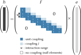
In the present framework of error correction of real-valued signals, the spatial coupling can be implemented by first constructing the matrix $F$ as the seeding matrix of [11], then determining the coding matrix $A$ as the null space of the matrix $F$. We refer to [11, 12, 13, 21] for a general discussion of spatial coupling in compressed sensing. The seeding measurement matrices $F_{\mu i}\in\mathbb{R}^{(M-N)\times N}$ that we use in the rest of this paper are constructed as in [12], see Fig. 2 for an example. The $M$ components of the error vector are sliced into $L_{c}$ equally-sized groups and the $M-N$ measurements into $L_{r}$ groups, the first of which having a larger number of measurements $m_{\rm seed}$ than the others $m_{\rm bulk}$. Define $\alpha_{\rm seed}=L_{c}m_{\rm seed}/M$ and $\alpha_{\rm bulk}=L_{c}m_{\rm bulk}/M$. Define $\alpha=(M-N)/M$ as the total measurement rate, we have $\alpha=[\alpha_{\rm seed}+(L_{r}-1)\alpha_{\rm bulk}]/L_{c}$. The matrix $F$ is then composed of $L_{r}\times L_{c}$ blocks where the elements $F_{\mu i}$ are generated independently, such that if $\mu$ is in group $q$ and $i$ in group $p$ then $F_{\mu i}$ is a random number with zero mean and variance $J_{q,p}/M$. In this work we use seeding matrices illustrated in Fig. 2 parameterized by $L$, $W$, and $J$.

Figure 2: Sketch of the seeding matrix $F$ we used to approach optimal reconstruction of the error vector with the AMP algorithm (see [12]). We use a number of variable-blocks $L_{c}=L$, and $L_{r}=L+1$ measurement blocks. The matrix components are iid with zero mean and variance $1/M$ for the blocks on the diagonal and for a number $W$ of lower diagonals, the upper diagonal blocks have components with variance $J/M$.

A rigorous analysis of the evolution of AMP reconstruction was performed for such matrices, assuming the knowledge of the $L_{r}\times L_{c}$ coupling matrix $J_{q,p}$ [17]. The state evolution for the block matrices can be done by defining $E_{p}^{t}$ to be the mean-squared error in block $p$ at time $t$. Then, $E_{p}^{t+1}$ depends on $\hat{m}_{p}^{t}$ from the same block according to eq. (13). The quantity $\hat{m}_{p}^{t}$ depends on the MSE $E^{t}_{q}$ from all the blocks $q=1,\dots,L_{c}$ as

$$\hat{m}_{p}^{t}=\frac{\alpha_{\rm seed}J_{1p}}{\sum_{q=1}^{L_{c}}J_{1q}E_{q}^{t}}+\alpha_{\rm bulk}\sum_{r=2}^{L_{r}}\frac{J_{rp}}{\sum_{q=1}^{L_{c}}J_{rq}E_{q}^{t}}\,.$$ (14)

This kind of state evolution belongs to the class for which threshold saturation (asymptotic achievement of performance matching the optimal Bayes estimation of the error) was proven in [22] (when $L\to\infty$, $W\to\infty$ and $L/W\gg 1$). It is also possible to compute the possible performance of Bayes-optimal reconstruction of the error analytically in the $N\to\infty$ limit as done in [12], and the results are shown again in Fig. 1 in green (upper-most) curve for $\epsilon=0$ and in red (2nd from top) curve for $\epsilon=10^{-6}$. The conclusion is that with the seeding matrices $F$, one can perform error correction using AMP up to these high coding rates.

Figure 3: Robustness to noise of the error correction for signal of size $N=256$. We compare the performances of the AMP-based and $\ell_{1}$ decoders, using $\epsilon=10^{-6}$ and homogeneous matrices $F$. The figure shows the probability density function (estimated with $500$ instances) of the robustness ratio eq. (15), called ${\hat{\rho}}_{\rm ideal}$ in [8] at different values of the coding rate $R$ and gross noise sparsity $\rho$. For coding rate $R=1/2$ and gross noise sparsity $\rho=0.1$, both methods (AMP in red and $\ell_{1}$ in black) are giving values close to one. However, AMP is better, on average it gives $0.89$ versus $0.74$ for $\ell_{1}$. Furthermore, AMP still performs very well when the fraction of gross errors is double (blue curve, with $\rho=0.2$) or when the coding rate $R$ is higher (green curve, with $R=2/3$). In both these cases, the $\ell_{1}$-based reconstruction gives poor results, an average value ${\hat{\rho}}_{\rm ideal}=37.1$ for $\rho=0.2$, $R=1/2$, versus $1.30$ for AMP; and ${\hat{\rho}}_{\rm ideal}=18.3$ for $\rho=0.1$, $R=2/3$, versus $1.20$ for AMP.

V Numerical tests

The asymptotic guarantees given in the last sections are encouraging, but evaluating analytically finite $M$ correction is intrinsically more difficult and hence we withdraw to numerical verifications of the achievable coding rates for sizes relevant for practical applications. Our Matlab code and demo are available on http://aspics.krzakala.org.

For numerical verifications, we used $N$-dimensional Gaussian signal x with zero mean and unit variance (the algorithm is not using this information) and a channel noise distributed according to eq. (1). We performed the Bayesian AMP algorithm to estimate the error $\hat{\textbf{e}}$. For exactly sparse channel, $\epsilon=0$, the exact reconstruction of e is possible and hence x can be recovered exactly. For approximately sparse channel, $\epsilon>0$, we use the AMP estimate of the error $\hat{\textbf{e}}$ to compute the estimate of $A\hat{\textbf{x}}$ and finally a pseudoinverse of $A$ to estimate the signal $\hat{\textbf{x}}$. We compare to the $\ell_{1}$ decoding approach (including the reprojection step) as developed in [7, 8].

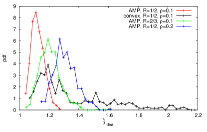
The data for $N\!=\!256$ are shown in Fig. 3 where the performance of our Bayes AMP decoding algorithm is compared to the $\ell_{1}$-based decoding of [8]. Following [8] we introduce an estimator of the robustness to noise called ${\hat{\rho}}_{\rm ideal}$ as the ratio of the MSE of the reconstructed signal $\hat{\textbf{x}}$ with the MSE of the ”ideal” reconstruction $\hat{\textbf{x}}_{\rm ideal}$, where the pseudoinverse of $A$ is applied to y that was corrupted only by the small additive noise without gross errors

$${\hat{\rho}}_{\rm ideal}=\frac{||\hat{\textbf{x}}-{\textbf{x}}||_{2}}{||\hat{\textbf{x}}_{\rm ideal}-{\textbf{x}}||_{2}}\,.$$ (15)

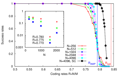
Fig. 3 depicts the histogram of ${\hat{\rho}}_{\rm ideal}$ over 500 random instances of the problem. We find that in all the cases we have tried with AMP (which were all in the favorable region of the asymptotic phase diagram), the robustness estimator ${\hat{\rho}}_{\rm ideal}$ is very close to unity, even at these relatively small sizes. Moreover the robustness estimator of AMP was always on average closer to unity than the one based on $\ell_{1}$ estimation and the distribution more peaked, thus demonstrating the advantage of the Bayesian AMP reconstruction in terms of performance, and noise robustness. Another important point is that the probability of a unsuccessful reconstruction is decaying exponentially fast when the system size increases. It is also decaying faster as $R$ decreases (see Fig. 4).

We also applied spatially coupled approach by choosing the matrix $F$ as described in Fig. 2 with $L=10$, $W=3$, $J=0.2$, $\alpha_{\rm seed}=0.22$, and varying $\alpha_{\rm bulk}$. While such parameters are far from the limit $L\to\infty$, $W\to\infty$, $W/L\to 0$ in which the optimal performance is guaranteed, we still obtain a considerable improvement in the achievable coding rate, as shown again in Fig. 4. In Fig. 5 we give a more visual illustration of the performance of the spatially coupled AMP decoder for $N=4096$. For gross error sparsity $\rho=0.1$ and small error variance $\epsilon=10^{-6}$ we were able to perform reliable error correction at coding rate $R=0.8$. This has to be compared with the original approach of [8] which only allows, even for infinite system sizes and in absence of small noise, an asymptotic $R\approx 0.67$.

Figure 4: Success rates of the decoding over $500$ instances for different signal sizes $N$ with noise parameters $\rho=0.1$, $\epsilon=10^{-6}$, both with seeding matrices $F$ (SC) and homogeneous random ones, as a function of the coding rate $R$. The vertical lines represent the limiting asymptotic coding rate for AMP with homogeneous and seeding matrices respectively. The maximum number of iterations in these simulations is set to $1000$. An instance is considered as successful if the final mean-squared-error of the reconstructed signal is less than $10^{-5}$. The inner plot shows the probability of failure that decays exponentially with the signal size for three different values of coding rate $R$.

Figure 5: Illustration of the error correcting scheme with the spatially coupled AMP approach and the $\ell_{1}$-based method of [8], applied to the benchmark Lena picture. The original $256\times 256$ image is decomposed in patches of size $N=64^{2}$. The noisy channel is given by eq. (1) using $\rho=0.1$, $\epsilon=10^{-6}$ and the coding rate is $R=0.796$ (to be compared with $R_{\rm opt}(\epsilon=10^{-6})=0.845$) is used together with spatially-coupled (seeded) matrix $F$ with parameters $L=10$, $W=3$, $J=0.2$, $\alpha_{\rm seed}=0.22$, $\alpha_{\rm bulk}=0.1830$.

VI Conclusion and perspectives

We have considered an error-correcting scheme for real-valued signals over channels that disrupt the transmitted signal by a large error on a small fraction of elements. We combined a Bayesian AMP reconstruction and spatially-coupled decoding matrices. We show that this approach is robust to non-sparse small noise, we computed the phase diagram in the limit of large signal sizes and showed numerically that the probability of failure decreases exponentially in the signal size.

There is a number of possible improvements on the present approach. First, the AMP approach is parallelizable, thus allowing substantial gain in execution time. One could also use structured $F$ matrices, for instance Fourrier, Gabor or Hadamard, as in [23], to further decrease the execution time of the AMP algorithm. Finally, another natural extension of the present work is when the signal x is itself compressible, so that a joint source and channel coding approach can be applied. We have done preliminary investigations on sparse signals in this direction.

References

- [1] A. Wyner, “An analog scrambling scheme which does not expand bandwidth, part i: Discrete time,” Information Theory, IEEE Transactions on, vol. 25, no. 3, pp. 261–274, 1979.
- [2] S. Feizi and M. Medard, “A power efficient sensing/communication scheme: Joint source-channel-network coding by using compressive sensing,” in Communication, Control, and Computing (Allerton), 2011 49th Annual Allerton Conference on. IEEE, 2011, pp. 1048–1054.
- [3] S. Shintre, S. Katti, S. Jaggi, B. Dey, D. Katabi, and M. Medard, “Real and complex network codes: Promises and challenges,” 2008.
- [4] M. Grangetto, P. Cosman, and G. Olmo, “Joint source/channel coding and map decoding of arithmetic codes,” Communications, IEEE Transactions on, vol. 53, no. 6, pp. 1007–1016, 2005.
- [5] G. Caire, T. Al-Naffouri, and A. Narayanan, “Impulse noise cancellation in ofdm: an application of compressed sensing,” in IEEE International Symposium on Information Theory Proceedings (ISIT), 2008, pp. 1293–1297.
- [6] D. Donoho and X. Huo, “Uncertainty principles and ideal atomic decomposition,” Information Theory, IEEE Transactions on, vol. 47, no. 7, pp. 2845–2862, 2001.
- [7] E. J. Candès and T. Tao, “Decoding by linear programming,” IEEE Trans. Inform. Theory, vol. 51, p. 4203, 2005.
- [8] E. J. Candes and P. A. Randall, “Highly robust error correction byconvex programming,” IEEE Trans. Inf. Theor., vol. 54, no. 7, pp. 2829–2840, Jul. 2008.
- [9] L. Lampe, “Bursty impulse noise detection by compressed sensing,” in Power Line Communications and Its Applications (ISPLC), 2011 IEEE International Symposium on. IEEE, 2011, pp. 29–34.
- [10] D. Donoho, A. Maleki, and A. Montanari, “Message passing algorithms for compressed sensing: I. motivation and construction,” in Information Theory Workshop (ITW), 2010 IEEE, 2010, pp. 1 –5.
- [11] F. Krzakala, M. Mézard, F. Sausset, Y. Sun, and L. Zdeborová, “Statistical physics-based reconstruction in compressed sensing,” Phys. Rev. X, vol. 2, p. 021005, 2012.
- [12] J. Barbier, F. Krzakala, M. Mézard, and L. Zdeborová, “Compressed sensing of approximately-sparse signals: Phase transitions and optimal reconstruction,” in 50th Annual Allerton Conference on Communication, Control, and Computing, 2012.
- [13] D. L. Donoho, A. Javanmard, and A. Montanari, “Information-theoretically optimal compressed sensing via spatial coupling and approximate message passing,” in IEEE International Symposium on Information Theory Proceedings (ISIT), 2012, pp. 1231–1235.
- [14] S. Rangan, “Generalized approximate message passing for estimation with random linear mixing,” in IEEE International Symposium on Information Theory Proceedings (ISIT), 31 2011-aug. 5 2011, pp. 2168 –2172.
- [15] F. Krzakala, M. Mézard, F. Sausset, Y. Sun, and L. Zdeborová, “Probabilistic reconstruction in compressed sensing: Algorithms, phase diagrams, and threshold achieving matrices,” J. Stat. Mech., vol. P08009, 2012.
- [16] M. Bayati and A. Montanari, “The dynamics of message passing on dense graphs, with applications to compressed sensing,” IEEE Transactions on Information Theory, vol. 57, no. 2, pp. 764 –785, 2011.
- [17] M. Bayati, M. Lelarge, and A. Montanari, “Universality in polytope phase transitions and message passing algorithms,” arXiv preprint arXiv:1207.7321, 2012.
- [18] S. Kudekar, T. Richardson, and R. Urbanke, “Spatially coupled ensembles universally achieve capacity under belief propagation,” in IEEE International Symposium on Information Theory Proceedings (ISIT), 2012, pp. 453–457.
- [19] S. Kudekar and H. Pfister, “The effect of spatial coupling on compressive sensing,” in Communication, Control, and Computing (Allerton), 2010, pp. 347–353.
- [20] D. L. Donoho and J. Tanner, “Sparse nonnegative solution of underdetermined linear equations by linear programming,” Proceedings of the National Academy of Sciences of the United States of America, vol. 102, no. 27, pp. 9446–9451, 2005.
- [21] M. C. Angelini, F. Ricci-Tersenghi, and Y. Kabashima, “Compressed sensing with sparse, structured matrices,” in Communication, Control, and Computing (Allerton), 2012 50th Annual Allerton Conference on, 2012, pp. 808–814.
- [22] A. Yedla, Y.-Y. Jian, P. S. Nguyen, and H. D. Pfister, “A simple proof of threshold saturation for coupled scalar recursions,” in 7th International Symposium on Turbo Codes and Iterative Information Processing (ISTC), 2012, pp. 51–55.
- [23] A. Javanmard and A. Montanari, “Subsampling at information theoretically optimal rates,” in IEEE International Symposium on Information Theory Proceedings (ISIT), 2012, pp. 2431–2435.