Obtaining the CMB anomalies with a bounce from the contracting phase to inflation
Abstract
Recent Planck data show the anomalies of CMB fluctuations on large angular scales, which confirms the early observations by WMAP. We continue studying an inflationary model, in which before the slow roll inflation the universe is in a contracting phase, and fit the model with the Planck data. It is showed that this model may generate not only the power deficit at low-, but also a large hemispherical power asymmetry in CMB. We also discuss the implication of the result to the eternal inflation scenario.
I Introduction
The inflation scenario is the current paradigm of the early universe. The inflation may be realized with the inflationary models, which will be identified by the observations. Recently, the Planck collaboration has released the data of the power on cosmic microwave background (CMB) [1],[2], which prefers the single field slow roll inflationary model with a concave potential.
However, the Planck collaboration has reported a power deficit in the low- CMB power spectrum at [3], which also is found in WMAP data, and not concordant with the Planck bestfit model, though the data points are still consistent well with the cosmic variance. Its statistical significance is about . In the meantime, the Planck collaboration has also reported a hemispherical power asymmetry in CMB [3], which conformed a similar result of WMAP [4, 5], but has better precision. The Planck data have larger statistical significance than in the WMAP data, which makes this asymmetry difficult to attribute the asymmetry to foregrounds.
These anomalies are actually intriguing, which has motivated some relevant studies. The curvaton scenario may explain the power asymmetry [6],[7],[8],[9],[10]. However, we will consider a different possibility, i.e. these anomalies might be a hint of the preinflationary physics. In this case, the inflation might last for just the minimum number of efoldings, the Planck bestfit single field inflationary model only actually provides a fit for the intermediate and small angular scales. After the WMAP1 data, the power deficit at low- has been investigated in Refs.[11],[12],[13],[14],[15],[17],[18] [19],[20],[21] along this line.
The study of the bouncing model has a long history, e.g.,Pre big-bang (PBB) scenario [22] and ekpyrotic scenario [23]. In the bouncing model, initially the universe is in a contracting phase, and then it bounces into an expanding phase, which results in a solution to the cosmological singularity problem. In Refs.[12],[13], the model, in which before the slow roll inflation the universe is in a contracting phase and after the bounce it begins to inflate, has been studied, which will be called the bouncing inflation model for simplicity here. In this model, the contracting phase is similar to that in PBB scenario, see [24],[25] for reviews, and in principle also may be that in ekpyrotic scenario. In the PBB scenario, the spectrum of the adiabatic perturbation generated during the kinetic contraction is highly blue, which is not consistent with the observations. However, here this blue spectrum is just required for the power suppression on large angular scale [12].
The slow roll inflation generally start in a high scale, which is required to insure that the amplitude of primordial perturbation is consistent with the observations and the reheating temperature is suitable with a hot big bang evolution after inflation. Recently, in the eternal inflation scenario, it has been argued that if the scale of the eternally inflating background is very low, the beginning of the slow roll inflation will requires a large uptunneling, which is exponentially unfavored. However, the introduction of the bounce before the slow roll inflation might significantly alter this result [26], and also [27],[28].
In Ref.[27], it is showed that in different cycle of cyclic universe, the universe may be in different minimum of a landscape, in which the bouncing inflation is responsible for the emergence of observational universe. In Ref.[29], it is showed that the inflation after bounce causes the cosmological hysteresis, which leads to the increase in the amplitude of cycles.
Thus whether theoretically or observationally, the studying of the bouncing inflation model is interesting. We will begin with a clarify of the primordial perturbation in this model in Sec.II. In Sec.III, we fit the model with the Planck data, and show that this model may generate the power deficit at low- and the hemispherical power asymmetry in CMB, which is consistent with the Planck data. The Sec.IV is the conclusion. We will briefly illustrate the model building and discuss the implication of the result to the eternal inflation scenario in the Appendix.
Note added: While this work is completed, Ref.[30] appeared, in which the authors discussed the effect of an instantaneous superinflationary phase after the bounce to the inflationary power spectrum.
II The primordial perturbation in bouncing inflation scenario
We will clarify the results of the primordial perturbation in bouncing inflation scenario. Here, we require that the bounce occurs at a higher scale than the inflationary scale and in the meantime all physical quantities continuously pass through the bounce. We will see that the result is insensitive with respect to implementing detail of the bounce.
The quadratic action of the curvature perturbation is
| (1) |
which is actually universal for single field, e.g. [31], where definition of is . The equation of in momentum space is [32],[33]
| (2) |
after is defined, where ′ is the derivative with respect to conformal time , . We have for canonical scalar field.
When , the perturbation mode is leaving the horizon. When , the solution of given by Eq.(2) is
| (3) | |||||
| (4) |
where the change of mode is dependent on the evolution of .
Before the bounce the universe is kinetic-dominated, whilst after the bounce it will get into an inflationary phase, we have , see Appendix for the detailed models. Thus in conformal time, after adopting an instantaneous matching between both regimes, we have
| (5) | |||||
where in the contracting phase and in the inflationary, respectively, and for is set, is the comoving Hubble length at matching time , which sets the inflationary energy scale by .
When , i.e. the perturbation is deep inside its horizon, oscillates with a constant amplitude,
| (6) |
In the contracting phase before inflation,
| (7) |
which will increase with time. When , i.e. the perturbation is far outside the horizon, the solution of Eq.(2) is
| (8) |
where is Hankel function of the first kind and of zeroth order.
In the inflationary phase,
| (9) |
When , the solution of Eq.(2) is
| (10) |
where is Hankel functions of the first kind and of order, and is Hankel functions of the second kind and of order, and are only dependent on .
When the bounce is nonsingular, all physical quantities should continuously pass through the bounce. The continuity of curvature perturbation brings
| (11) | |||||
| (12) | |||||
where is Hankel functions of the second kind and of zeroth order, and is Hankel functions of the second kind and of first order.
The spectrum of is
| (13) |
We substitute Eq.(10) into (13), and have the spectrum of curvature perturbation
| (14) | |||||
| (15) |
where is that of the standard slow roll inflation, which may has a slight red spectrum consistent with the observation, and are determined by Eqs. (11) and (12), respectively. Here, we have expanded and in term of , and used
Here, is the comoving Hubble length at matching time , which implies that for is given in the contracting phase, while for is in the inflationary phase. In and , the Hankel functions are the function of . We can expand the Hankel functions in term of and have approximately
| (16) | |||||
Thus on the scale , the spectrum is strongly blue , which is the usual result of PBB scenario. While for , we have
| (17) |
which is almost scale invariant but modulated with a small oscillation. The scale invariance of spectrum is actually the result of inflationary evolution after the bounce. The reason is in the contracting phase the perturbation mode with is still inside the horizon, and its evolution is determined by Eq.(6) and is insensitive to the background at this stage, only when the corresponding perturbation mode leaves the horizon, which occurs in the inflationary phase, the perturbation spectrum is determined by the evolution of the background.
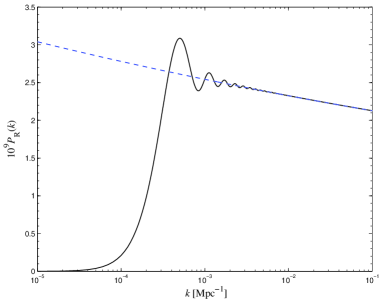
We plot in (14) as a function of in Fig.1. We see that for , the spectrum is almost scale invariant with a slightly red tilt and an oscillation with a decaying amplitude, and for the amplitude of spectrum decreases rapidly and gets a cutoff, which is consistent with our analytical results (16) and (17).
III The CMB anomalies with Planck
III.1 The power deficit in low-
In Eq.(14), may be parameterized as a power law with
| (18) |
Here we emphasize that in terms of this definition, the spectral index of curvature perturbation defined in Eq.(15) is for and for . Thus the primordial spectrum (14) is described by three free parameters, {,,}. The pivot scale, , is chosen to be Mpc-1, roughly in the middle of the logarithmic range of scales probed by Planck. In addition, cosmological evolution at late times can be characterized by four free parameters, {}, where is the dimensionless Hubble parameter such that kms-1 Mpc-1, and are the physical baryon and dark matter densities relative to the critical density, is the ratio of the sound horizon to the angular diameter distance at the photon decoupling, and is the reionization optical depth. We impose a uniform prior on the logarithm of in the range . For the other parameters, prior ranges are chosen to be much larger than the posterior. In order to compute the theoretical CMB power spectrum, we modify the Boltzmann CAMB code in [34]. In Fig. 2 we plot the angular power spectrum for the pure power law (dashed) and bouncing inflation with the best-fit value of (solid). Compared to the standard power-law model, the spectrum in the bouncing Universe is suppressed in the quadrupole and octupole. Moreover, a small bump around arises from the oscillations of the primordial power spectrum at large scales.
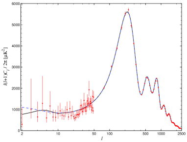
We use the combination of the Planck CMB temperature power spectrum [1, 2] with the WMAP large-scale polarization data [35] (denoted “Planck+WP”). The Planck temperature likelihood is based on a hybrid approach, which combines a pixel-based likelihood at low multipoles () with a Gaussian likelihood approximation at high multipoles (). The Planck high- likelihood involves 14 nuisance parameters to describe unresolved small-scale foreground and CMB secondary anisotropies. Since Planck doesn’t release polarization data, the WMAP polarization data at low multipoles () is used to constrain the optical depth.
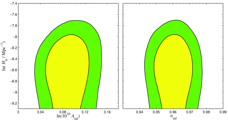
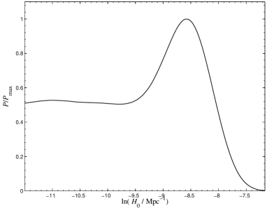
In our analysis we use a modified version of the publicly available CosmoMC package to explore the parameter space by means of Monte Carlo Markov chains technique [36]. From the Planck+WP data we find the best-fit values of , and with . This indicates that the bouncing inflation model can improve the fit to the data with with respect to the standard power-law model. However, a phenomenological exponential-form cutoff of the primordial power spectrum improves the fit only with reported in [2]. Moreover, the exponential-form cutoff in [2] is described by two parameters, the cutoff steepness and the cutoff scale . In the bouncing inflation model, the cutoff is characterized by only one parameter . We show the joint constraints on , and in Fig. 3. Since characterizes local features in the power spectrum while and characterize the global shape of the power spectrum (see [37] for a general shape reconstructed from CMB data), there is nearly no correlation between them, as shown in Fig. 3. The marginalized posterior distribution of is shown in Fig. 4, which illustrates the asymmetric shape of the likelihood functions.
III.2 The hemispherical power asymmetry
Recently, the Planck collaboration has reported a hemispherical power asymmetry in CMB [3], which conformed a similar result of WMAP [4], but has better precision. It could be thought that this power asymmetry might result from a superhorizon perturbation crossing the observable universe. We will estimate the hemispherical power asymmetry in the bouncing inflation, along the line of Ref.[6] by Erickcek et.al and Ref.[7] by Lyth.
The CMB power asymmetry might be modeled as a dipole modulation of the power [38],[39],[40]. This modulation can be explained in light of the spatial change of the power spectrum of primordial curvature perturbation ,
| (19) |
where is the amplitude of the modulation, the unit vector is the dipole modulation direction, is the distance to the last scattering surface, and is given by Eq.(14).
The asymmetry can be calculated as,
| (20) | |||||
where is the amplitude of the power spectrum of a single modulating mode , i.e.,
| (21) |
and for this modulating mode we have . Here, for the contracting phase and for the inflationary phase. The inflationary result is recovered for [6],[7]. Here, arises from the dependence of on the time in Eq.(15), since .
The maximum achievable value of is given by the limits on the terms on the right-hand side of Eq.(20). The perturbation amplitude of the superhorizon mode with can be constrained by its contribution to the CMB quadrupole, i.e., the Grishchuk-Zel’dovich effect. This has been computed using the Sachs-Wolfe approximation in Ref.[7] as
| (22) | |||||
In deriving the second line of (22) we have used Eq.(21). Requiring to be the measured rms value of the quadrupole, we have
| (23) |
which gives , since for the perturbation theory to apply. Plugging this result into Eq.(20), we have an upper bound on the modulation amplitude of the CMB power asymmetry,
| (24) |
This amplitude is measured to be from the 5-year WMAP analyses [5], which is consistent with the Planck results [3].
In single field inflationary scenario, and . Thus we have , which is too small to fit the observation, as pointed out in Refs. [6],[7]. However, the case is altered in curvaton scenario, see [7],[8].
In bouncing inflation scenario discussed here, on large angular scale , the curvature perturbation origins from the fluctuation of during the contraction. We have and , as have been calculated in Sec.II. Thus in this scenario the power asymmetry on large angular scale is
| (25) |
which is consistent with Planck data. The power spectrum at intermediate and small angular scales is that of slow roll inflation, thus the corresponding power asymmetry is small, which is consistent with the constraint from the SDSS sample of quasars [41].
Here, (25) applies only to scales , while the required range is 444We thank David H. Lyth for pointing out this to us.. Our best-fit value is , which corresponds to , since the distance to the last scattering surface is estimated as . This result seems to imply that our model has a tension with the observation. However, as shown in Fig.3, at confidence level may be , and further, at which though was not plotted, it may be . Thus our model is consistent with Planck’s constraints at . The observation has placed strong constraints on our model, which makes it easily falsified by further Planck data.
IV Conclusion
Recently, the Planck collaboration has released the data of the power on cosmic microwave background, which is consistent with the slow roll inflationary model. However, the Planck data also show a power deficit at and a hemispherical power asymmetry in CMB, which conformed the early observations by WMAP. This result is intriguing, since it might be a hint of the physics at the epochs before the inflation.
We continue studying the bouncing inflation model. In this model, we assume that initially the universe is in a contracting phase, and after the bounce it begins to inflate. The contraction before the bounce leads to that the primordial power spectrum on large angular scales has the spectral index , where is a new degree of freedom, which sets the cutoff scale. We find that this spectrum generates not only the power deficit at low-l, but also the hemispherical power asymmetry in CMB, which may be consistent with the Planck data. Thus our model can explain the CMB anomalies, which may be falsified by further Planck data.
The bouncing inflation model not only sets a natural initial condition for the beginning of the slow roll inflation, significantly but also is connected with the preinflationary physics. We discussed the model building in the Appendix. It is interesting to embed a bouncing model into a fundamental theory. In principle, depending on the implemented detail of the bounce, the models may be different. However, these details do not quanlitatively affect the result of the primordial spectrum given here.
We also showed that in the eternal inflation scenario, the bouncing inflation might be a favored channel to implement the slow roll inflation. Thus it is interesting to have a detailed study in a string landscape motivated well.
Acknowledgments
We thank David H. Lyth for helpful discussions. ZKG is supported by the project of Knowledge Innovation Program of Chinese Academy of Science, NSFC under Grant No.11175225, and National Basic Research Program of China under Grant No.2010CB832805. YSP is supported by NSFC under Grant No.11075205, 11222546, and National Basic Research Program of China, No.2010CB832804. We used CosmoMC and CAMB. We acknowledge the use of the Planck data and the Lenovo DeepComp 7000 supercomputer in SCCAS.
Appendix A: The models of bouncing inflation
In this Appendix, we will discuss some models of the bouncing inflation.
The Lagrangian is
| (26) |
where the potential is only the function of the field . Here, we regard the potential as
| (27) |
This potential is a Higgslike potential for the parameters , and . While for and , this potential corresponds to that from the minimal supersymmetric standard model e.g.[42]. There might be two or three minima in this potential, dependent of the values of parameters, see Fig.5.
Here, is the ghost field, whose only role is to simply implement the bounce. In principle, the ghost instability may be dispelled by applying the Galileon interaction [43]. The bounce may be also implemented like in e.g.[24],[25] for PBB scenario, [23] for ekpyrotic scenario. The Lagrangian of is specially selected for convenience, since it may lead to an analytical solution of around the bounce.
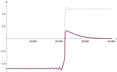
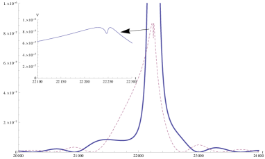
We plot the evolution of , and in Fig.6 for the potential in the upper panel of Fig.5, and the evolutions of , the kinetic energy and the potential energy in Figs.7 and 8 for the potential in the lower panel of Fig.5. The universe initially is in a contracting phase, and the field is in one among the minima of its potential. We see that before the bounce, the field will climb up along its potential [12],[44], and its kinetic energy will become dominated, while after the bounce, the kinetic energy of will be rapidly diluted and the universe will get into an inflationary phase, and finally the field will roll down along the potential to the other minima. Here, the contracting phase actually provides a homogeneous patch for the beginning of slow roll inflation, which helps to relax the initial conditions problem argued in Ref.[46].
The Lagrangian of implies . When is dominated, we have for field. Thus the Friedmann equation is
| (28) |
Thus we have
| (29) |
There is a bounce at , while when deviates from , which is consistent with Fig.6.
The field will walk with certain distance during is dominated, before it finally lands in an inflationary region. Here, “land” means that the effective potential of field begins to become dominated. The change of before the field lands is . We have , which gives [29],[45]
| (30) |
where for is applied, and is the Hubble parameter before and after the bounce and is that at the time when the kinetic energy of field begins to dominate. We generally have , which implies .


Appendix B: The implication for the eternal inflation scenario
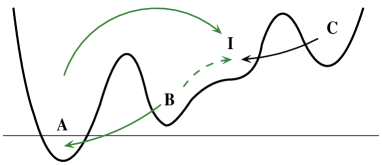
In the eternal inflation scenario [47], an infinite number of universes will be spawned in the eternally inflating background. It might be thought that a phase of the slow roll inflation and reheating is required for a spawned universe becoming our observable universe.
The slow roll inflation should start in a high scale, which is required to insure that the amplitude of primordial perturbation is consistent with the observations and the reheating temperature is suitable for a hot big bang model. In this sense, if the scale of the eternally inflating background is very low, the spawning of observational universe will requires a large uptunneling, which is exponentially unfavored.
However, the introduction of the nonsingular bounce might significantly alter this result [26],[27],[28]. Here, we will briefly revisit this issue with the bouncing inflation. We will show that the bouncing inflation is a favored channel to the slow roll inflation in a given landscape.
In a landscape of the effective potential in Fig.9, we have a AdS minimum ‘A’, a dS minimum ‘B’ with lower energy, a dS minimum with higher energy and a slow-roll inflationary region ‘I’. The transitions in this landscape are ‘B’ ‘A’, ‘B’ ‘I’ and ‘I’ ‘C’. In addition, ‘I’ may also classically roll into ‘B’, and the AdS crunch in ‘A’ is replaced with the bounce, and the corresponding probabilities of bouncing to ‘B’, ‘C’ and ‘I’ are , and , respectively, with .
We follow Ref.[48]. The rate equation describing the fractions in corresponding regions is , where
| (31) |
| (32) |
where is the transition rate, and is the nucleation rate of bubble, and , is the time the slow roll inflation lasts and is the efolds number. The distributions will be fixed at late time. Thus we have
| (33) | |||||
| (34) | |||||
where and are used. We have
| (35) |
which is consistent with the result of Garriga and Vilenkin [26], i.e. the ratio is not suppressed by the small uptunnelling rate.
Here, we are interested in the ratio of probabilities of the different channels to the slow-roll inflationary region. Here, one channel is the AdS bounce from ‘A’, the others are the uptunnelling from ‘B’ and the tunnelling from ‘C’. We have, after noting the corresponding terms with a plus sign at the right side of the equation in Eqs.(32),
| (36) | |||||
| (37) | |||||
| (38) |
for these channels, respectively, in which denotes the incoming probability current into the slow roll inflationary region, as defined in [49], and the subscript “Ainf” denotes that from ‘A’ into the inflationary region. Thus the ratio of to is given by
| (39) |
where we have made the integral for both sides of Eq.(33), and substituted it into this equation. We generally have , since is that of the uptunnelling. Thus Eq.(39) implies that, compared with the channel of uptunnelling to slow roll inflation, the bouncing inflation is favored exponentially.
The ratio of to is given similarly by
| (40) |
Thus in a given landscape, the bouncing inflation and the inflationary bubble from ‘C’ have almost equal possibility. However, it should be noticed that in Eq.(34), if is negligible, we will have , in which is the contribution from the AdS bounce.
References
- [1] P. A. R. Ade et al. [ Planck Collaboration], arXiv:1303.5062 [astro-ph.CO].
- [2] P. A. R. Ade et al. [Planck Collaboration], arXiv:1303.5082 [astro-ph.CO].
- [3] P. A. R. Ade et al. [Planck Collaboration], arXiv:1303.5083 [astro-ph.CO].
- [4] H. K. Eriksen, A. J. Banday, K. M. Gorski, F. K. Hansen and P. B. Lilje, Astrophys. J. 660, L81 (2007) [astro-ph/0701089].
- [5] J. Hoftuft, H. K. Eriksen, A. J. Banday, K. M. Gorski, F. K. Hansen and P. B. Lilje, Astrophys. J. 699, 985 (2009) [arXiv:0903.1229 [astro-ph.CO]].
- [6] A. L. Erickcek, M. Kamionkowski and S. M. Carroll, Phys. Rev. D 78, 123520 (2008) [arXiv:0806.0377 [astro-ph]].
- [7] D. H. Lyth, arXiv:1304.1270 [astro-ph.CO].
- [8] L. Wang and A. Mazumdar, arXiv:1304.6399 [astro-ph.CO].
- [9] J. McDonald, arXiv:1305.0525 [astro-ph.CO].
- [10] M. H. Namjoo, S. Baghram and H. Firouzjahi, arXiv:1305.0813 [astro-ph.CO].
- [11] C. R. Contaldi, M. Peloso, L. Kofman and A. D. Linde, JCAP 0307, 002 (2003) [astro-ph/0303636]; G. Nicholson and C. R. Contaldi, JCAP 0801, 002 (2008) [astro-ph/0701783].
- [12] Y. -S. Piao, B. Feng and X. -m. Zhang, Phys. Rev. D 69, 103520 (2004) [hep-th/0310206]; Y. -S. Piao, Phys. Rev. D 71, 087301 (2005) [astro-ph/0502343].
- [13] Y. -S. Piao, S. Tsujikawa and X. -m. Zhang, Class. Quant. Grav. 21, 4455 (2004) [hep-th/0312139].
- [14] B. A. Powell and W. H. Kinney, Phys. Rev. D 76, 063512 (2007) [astro-ph/0612006].
- [15] D. Boyanovsky, H. J. de Vega and N. G. Sanchez, Phys. Rev. D 74, 123006 (2006) [astro-ph/0607508]; D. Boyanovsky, H. J. de Vega and N. G. Sanchez, Phys. Rev. D 74, 123007 (2006) [astro-ph/0607487];
- [16] C. Destri, H. J. de Vega and N. G. Sanchez, Phys. Rev. D 78, 023013 (2008) [arXiv:0804.2387 [astro-ph]]; D. Boyanovsky, C. Destri, H. J. De Vega and N. G. Sanchez, Int. J. Mod. Phys. A 24, 3669 (2009) [arXiv:0901.0549 [astro-ph.CO]].
- [17] J. Mielczarek, JCAP 0811, 011 (2008) [arXiv:0807.0712 [gr-qc]]; J. Mielczarek, M. Kamionka, A. Kurek and M. Szydlowski, JCAP 1007, 004 (2010) [arXiv:1005.0814 [gr-qc]].
- [18] M. J. Mortonson and W. Hu, Phys. Rev. D 80, 027301 (2009) [arXiv:0906.3016 [astro-ph.CO]].
- [19] J. Liu, Y. -F. Cai and H. Li, J. Theor. Phys. 1, 1 (2012) [arXiv:1009.3372 [astro-ph.CO]].
- [20] E. Dudas, N. Kitazawa, S. P. Patil and A. Sagnotti, JCAP 1205, 012 (2012) [arXiv:1202.6630 [hep-th]].
- [21] M. Bouhmadi-Lopez, P. Chen, Y. -C. Huang and Y. -H. Lin, arXiv:1212.2641 [astro-ph.CO].
- [22] M. Gasperini and G. Veneziano, Astropart. Phys. 1 317 (1993).
- [23] J. Khoury, B. A. Ovrut, P. J. Steinhardt and N. Turok, Phys. Rev. D 64, 123522 (2001) [hep-th/0103239]; E. I. Buchbinder, J. Khoury and B. A. Ovrut, Phys. Rev. D 76, 123503 (2007) [hep-th/0702154];
- [24] M. Gasperini, G. Veneziano, Phys. Rept. 373, 1 (2003).
- [25] J.E. Lidsey, D. Wands and E.J. Copeland, Phys. Rept. 337, 343 (2003).
- [26] J. Garriga and A. Vilenkin, arXiv:1210.7540 [hep-th]; A. Vilenkin, AIP Conf. Proc. 1514, 7 (2012) [arXiv:1301.0121 [hep-th]].
- [27] Y. -S. Piao, Phys. Rev. D 70, 101302 (2004) [hep-th/0407258]; Y.S. Piao, Phys. Lett. B677, 1 (2009); Phys. Lett. B691, 225 (2010).
- [28] M. C. Johnson and J. -L. Lehners, Phys. Rev. D 85, 103509 (2012) [arXiv:1112.3360 [hep-th]]; J. -L. Lehners, Phys. Rev. D 86, 043518 (2012) [arXiv:1206.1081 [hep-th]].
- [29] V. Sahni and A. Toporensky, Phys. Rev. D 85, 123542 (2012) [arXiv:1203.0395 [gr-qc]].
- [30] T. Biswas and A. Mazumdar, arXiv:1304.3648 [hep-th].
- [31] J. Garriga, V.F. Mukhanov, Phys. Lett. B458, 219 (1999).
- [32] V.F. Mukhanov, JETP lett. 41, 493 (1985); Sov. Phys. JETP. 68, 1297 (1988).
- [33] H. Kodama, M. Sasaki, Prog. Theor. Phys. Suppl. 78 1 (1984).
- [34] A. Lewis, A. Challinor and A. Lasenby, Astrophys. J. 538, 473 (2000) [arXiv:astro-ph/9911177].
- [35] L. Page et al. [WMAP Collaboration], Astrophys. J. Suppl. 170, 335 (2007) [astro-ph/0603450].
- [36] A. Lewis and S. Bridle, Phys. Rev. D 66, 103511 (2002) [arXiv:astro-ph/0205436]; A. Lewis, Phys. Rev. D87, 103529 (2013) [arXiv:1304.4473].
- [37] Z. K. Guo, D. J. Schwarz and Y. Z. Zhang, JCAP 1108, 031 (2011) [arXiv:1105.5916]; Z. K. Guo and Y. Z. Zhang, JCAP 1111, 032 (2011) [arXiv:1109.0067]; Z. K. Guo and Y. Z. Zhang, Phys. Rev. D 85, 103519 (2012) [arXiv:1201.1538].
- [38] S. Prunet, J. -P. Uzan, F. Bernardeau and T. Brunier, Phys. Rev. D 71, 083508 (2005) [astro-ph/0406364].
- [39] C. Gordon, W. Hu, D. Huterer and T. M. Crawford, Phys. Rev. D 72, 103002 (2005) [astro-ph/0509301].
- [40] C. Gordon, Astrophys. J. 656, 636 (2007) [astro-ph/0607423].
- [41] C. M. Hirata, JCAP 0909, 011 (2009) [arXiv:0907.0703[astro-ph.CO]].
- [42] R. Allahverdi, K. Enqvist, J. Garcia-Bellido, A. Jokinen and A. Mazumdar, JCAP 0706, 019 (2007) [hep-ph/0610134].
- [43] T. Qiu, J. Evslin, Y.F. Cai, M.Z. Li, X.M. Zhang, JCAP 1110, 036 (2011); D.A. Easson, I. Sawicki, A. Vikman, JCAP 1111, 021 (2011); M. Osipov and V. Rubakov, arXiv:1303.1221; T. Qiu, X. Gao and E. N. Saridakis, arXiv:1303.2372; D.A. Easson, I. Sawicki, A. Vikman, arXiv:1304.3903.
- [44] N. Kanekar, V. Sahni and Y. Shtanov, Phys. Rev. D 63, 083520 (2001) [astro-ph/0101448].
- [45] Y. -S. Piao and Y. -Z. Zhang, Nucl. Phys. B 725, 265 (2005) [gr-qc/0407027].
- [46] A. Ijjas, P. J. Steinhardt and A. Loeb, arXiv:1304.2785 [astro-ph.CO].
- [47] A. Vilenkin, Phys. Rev. D27, 2848 (1983); A.D. Linde, Phys. Lett. B175, 395 (1986); P.J. Steinhardt, in “The Very Early Universe”, ed. by G.W. Gibbons, S.W. Hawking and S.T.C. Siklos (Cambridge University Press, 1983).
- [48] J. Garrige and A. Vilenkin, Phys. Rev. D57, 2230 (1998).
- [49] A. D. Linde, JCAP 0701, 022 (2007) [hep-th/0611043].