Numerical Integration of the Extended Variable Generalized Langevin Equation with a Positive Prony Representable Memory Kernel

Abstract

Generalized Langevin dynamics (GLD) arise in the modeling of a number of systems, ranging from structured fluids that exhibit a viscoelastic mechanical response, to biological systems, and other media that exhibit anomalous diffusive phenomena. Molecular dynamics (MD) simulations that include GLD in conjunction with external and/or pairwise forces require the development of numerical integrators that are efficient, stable, and have known convergence properties. In this article, we derive a family of extended variable integrators for the Generalized Langevin equation (GLE) with a positive Prony series memory kernel. Using stability and error analysis, we identify a superlative choice of parameters and implement the corresponding numerical algorithm in the LAMMPS MD software package. Salient features of the algorithm include exact conservation of the first and second moments of the equilibrium velocity distribution in some important cases, stable behavior in the limit of conventional Langevin dynamics, and the use of a convolution-free formalism that obviates the need for explicit storage of the time history of particle velocities. Capability is demonstrated with respect to accuracy in numerous canonical examples, stability in certain limits, and an exemplary application in which the effect of a harmonic confining potential is mapped onto a memory kernel.

Copyright 2013 American Institute of Physics. This article may be downloaded for personal use only. Any other use requires prior permission of the author and the American Institute of Physics.

I Introduction

Langevin dynamicsCoffey, Kalmykov, and Waldron (2004) is a modeling technique, in which the motion of a set of massive bodies in the presence of a bath of smaller solvent particles is directly integrated, while the dynamics of the solvent are “averaged out”. This approximation may lead to a dramatic reduction in computational cost compared to “explicit solvent” methods, since dynamics of the solvent particles no longer need to be fully resolved. With Langevin dynamics, the effect of the solvent is reduced to an instantaneous drag force and a random delta-correlated force felt by the massive bodies. This framework has been applied in a variety of scenarios, including implicit solvents,Uhlenbeck and Ornstein (1930); Kubo (1966) Brownian dynamics,Ermak and McCammon (1978) dynamic thermostats,Schneider and Stoll (1978) and the stabilization of time integrators.Izaguirre et al. (2001)

In spite of the numerous successes of conventional Langevin dynamics it has long been recognized that there are physically compelling scenarios in which the underlying assumptions break down, necessitating a more general treatment.Mori (1965a); Kubo (1966) To this end, generalized Langevin dynamics (GLD) permits the modeling of systems in which the inertial gap separating the massive bodies from the smaller solvent particles is reduced. Here the assumptions of an instantaneous drag force and a delta-correlated random force become insufficient, leading to the introduction of a temporally non-local drag and a random force with non-trivial correlations. GLD has historically been applied to numerous problems over the years,Doll and Dion (1976); Shugard, Tully, and Nitzan (1977); Toxvaerd (1987); Schweizer (1989) with a number of new applications inspiring a resurgence of interest, including microrheology,Mason and Weitz (1995); Mason, Gang, and Weitz (1997); Fricks et al. (2009); Didier et al. (2012) biological systems,Kou and Xie (2004); Min et al. (2005); Gordon, Krishnamurthy, and Chung (2009) nuclear quantum effects,Ceriotti, Bussi, and Parrinello (2009, 2009); Ceriotti and Manolopoulos (2012) and other situations in which anomalous diffusion arises.Sokolov (2012)

To facilitate computational exploration of some of these applications, a number of authors have developed numerical integration schemes for the generalized Langevin equation (GLE), either in isolation or in conjunction with extra terms accounting for external or pairwise forces as would be required in a molecular dynamics (MD) simulation. These schemes must deal with a number of complications if they are to remain computationally efficient and accurate.

• The retarded drag force takes the form of a convolution of the velocity with a memory kernel. This requires the storage of the velocity history, and the numerical evaluation of a convolution at each time step, which can become computationally expensive.

• The generation of a random force with non-trivial correlations may also require the storage of a sequence of random numbers, and some additional computational expense incurred at each time step.

Numerous methods exist that circumvent either one or both of these difficulties.Doll and Dion (1976); Ciccotti and Ryckaert (1980); Berkowitz, Morgan, and McCammon (1983); Guàrdia and Padró (1985); Straub, Borkovec, and Berne (1986); Smith and Harris (1990); Nilsson and Padró (1990); Wan, Wang, and Shi (1998); Gordon, Krishnamurthy, and Chung (2008) Each has a different computational cost, implementation complexity, order of convergence, and specific features, e.g., some are restricted to single exponential memory kernels, require linear algebra, etc. To this end, it is difficult to distinguish any individual method as being optimal, especially given the broad range of applications to which GLD may be applied.

Motivated by the aforementioned applications and previous work in numerical integrators, we have developed a new family of time integration schemes for the GLE in the presence of conservative forces, and implemented it in a public domain MD code, LAMMPS.Plimpton (1995) Our primary impetus was to enable the development of reduced order models for nanocolloidal suspensions, among a variety of other applications outlined above. Previous computational studies of these systems using explicit solvents have demonstrated and resolved a number of associated computational challenges. in ’t Veld (2008) Our method enables a complementary framework for the modeling of these types of systems using implicit solvents that can include memory effects. Otherwise, to date the GLE has only been solved in the presence of a number of canonically tractable external potentials and memory kernels.Kou and Xie (2004); Despósito and Viñales (2009); Viñales and Despósito (2006) Integration into the LAMMPS framework, provides a number of capabilities. LAMMPS includes a broad array of external, bonded, and non-bonded potentials, yielding the possibility for the numerical exploration of more complex systems than have been previously studied. Finally, LAMMPS provides a highly scalable parallel platform for studying N-body dynamics. Consequently, extremely large sample statistics are readily accessible even in the case of interacting particles, for which parallelism is an otherwise non-trivial problem.

In this paper, details germane to both the development of our time integration scheme, as well as specifics of its implementation are presented. The time integration scheme to be discussed is based upon a two-parameter family of methods specialized to an extended variable formulation of the GLE. Some of the salient advantages of our formulation and the final time integration scheme are:

• Generalizability to a wide array of memory kernels representable by a positive Prony series, such as power laws.

• Efficiency afforded by an extended variable formulation that obviates the explicit evaluation of time convolutions.

• Inexpensive treatment of correlated random forces, free of linear algebra, requiring only one random force evaluation per extended variable per timestep.

• Exact conservation of the first and second moments of either the integrated velocity distribution or position distribution, for harmonically confined and free particles.

• Numerically stable approach to the Langevin limit of the GLE.

• Simplicity of implementation into an existing Verlet MD framework.

The specialization to Prony-representable memory kernels is worth noting, as there is a growing body of literature concerning this form of the GLE.Fricks et al. (2009); McKinley, Yao, and Gregory (2009); Ottobre and Pavliotis (2011) A number of results have been presented that establish the mathematical well-posedness of this extended variable GLE including a term accounting for smooth conservative forces, as may arise in MD.Ottobre and Pavliotis (2011) These results include proofs of ergodicity and exponential convergence to a measure, as well as a discussion of the Langevin limit of the GLE in which the parameters of the extended system generate conventional Langevin dynamics.

One somewhat unique feature of our framework is that we are analyzing the GLE using methods from stochastic calculus. In particular, we focus on weak convergence in the construction our method, i.e., error in representing the moments of the stationary distribution or the distribution itself. The optimal parametrization of our two-parameter family of methods will be defined in terms of achieving accuracy with respect to this type of convergence. In particular, the optimal method that has been implemented achieves exactness in the first and second moments of the integrated velocity distribution for harmonically confined and free particles. Few authors have considered this type of analysis for even conventional Langevin integrators, with a notable exception being Wang and Skeel,Wang and Skeel (2003) who have carried out weak error analysis for a number of integrators used in conventional Langevin dynamics. To the best of our knowledge, this is the first time that such a weak analysis has been carried out for a GLE integrator. We hope that these considerations will contribute to a better understanding of existing and future methods.

The remainder of this paper is structured as follows:

• Section II.1 introduces the mathematical details of the GLE.

• Section II.2 presents the extended variable formulation and its benefits.

• Section II.3 develops the theory associated with integrating the extended variable GLE in terms of a two-parameter family of methods.

• Section II.4 provides details of the error analysis that establishes the ‘optimal’ method among this family.

• Section II.5 discusses the extension of our method to a multi-stage splitting framework.

• Section III summarizes details of the implementation in LAMMPS.

• Section IV presents a number of results that establish accuracy in numerous limits/scenarios, including demonstration of utility in constructing reduced order models.

II Mathematical Details

II.1 Statement of the Problem

The GLE for $N_{p}$ particles moving in $d$-dimensions can be written as

$$MdV(t)=F^{c}\left(X(t)\right)dt-\int\limits_{0}^{t}\Gamma(t-s)V(s)dsdt+F^{r}(t)dt,$$ (1a)

$$dX(t)=V(t)dt,$$ (1b)

with initial conditions $X(0)=X_{0}$ and $V(0)=V_{0}$. Here, $F^{c}:\mathbb{R}^{dN_{p}}\rightarrow\mathbb{R}^{dN_{p}}$ is a conservative force, $F^{r}$ is a random force, $M$ is a diagonal mass matrix, and $\Gamma$ is a memory kernel. The solution to this stochastic integro-differential equation is a trajectory, which describes the positions $X:\mathbb{R}^{+}\rightarrow\mathbb{R}^{dN_{p}}$ and velocities $V:\mathbb{R}^{+}\rightarrow\mathbb{R}^{dN_{p}}$ of the particles as a function of time, $t\geq 0$. The second term on the right-hand side of Equation 1a accounts for the temporally non-local drag force, and the third term accounts for the correlated random force. The nature of both forces are characterized by the memory kernel, $\Gamma:\mathbb{R}^{+}\rightarrow\mathbb{R}$, consistent with the Fluctuation-Dissipation theorem (FDT).Kubo (1966); Callen and Welton (1951) The FDT states that equilibration to a temperature, T, requires that the two-time correlation of $F^{r}(t)$ and $\Gamma(t)$ be related as follows:

$$\langle F^{r}_{i}(t+s)F^{r}_{j}(t)\rangle=\text{k}_{B}\text{T}\,\Gamma(s)\delta_{ij},\quad s\geq 0.$$ (2)

Here, $\delta_{ij}$ is the Kronecker delta, and $\text{k}_{B}$ is Boltzmann’s constant.

In the context of an MD simulation, we are interested in solving Equation 1 for both $X(t)$ and $V(t)$ at a set of $N_{t}$ uniformly spaced discrete points in time. To this end, we seek to construct a solution scheme that is mindful of the following complications:

• Calculation of the temporally non-local drag force requires a convolution with $\Gamma(t)$, and thusly the storage of some subset of the time history of $V(t)$.

• Numerical evaluation of $F^{r}(t)$ requires the generation of a sequence of correlated random numbers, as specified in Equation 2.

• As Equation 1 is a stochastic differential equation (SDE), we are not concerned with issues of local or global error, but rather that the integrated solution converges in distribution.

To circumvent the first two complications, we work with an extended variable formalismFricks et al. (2009); Mori (1965b); Ceriotti, Bussi, and Parrinello (2009); Kupferman (2004) in which we assume that $\Gamma(t)$ is representable as a Prony series:

$$\Gamma(t)=\sum\limits_{k=1}^{N_{k}}\frac{c_{k}}{\tau_{k}}\text{exp}\left[-\frac{t}{\tau_{k}}\right],\quad t\geq 0.$$ (3)

As will be demonstrated in Section II.2, this form of the memory kernel will allow us to map the non-Markovian form of the GLE in Equation 1 onto a higher-dimensional Markovian problem with $dN_{k}$ extended variables per particle. The third complication is resolved in Sections II.3 and II.4, in which a family of integrators is derived, and then ‘optimal’ parameters are selected based upon an error analysis of the moments of the integrated velocity.

II.2 Extended Variable Formalism

We introduce the extended variable formalism in two stages. First, we define a set of extended variables that allow for an effectively convolution-free reformulation of Equation 1. Then, we demonstrate that the non-trivial temporal correlations required of $F^{r}(t)$ can be effected through coupling to an auxiliary set of Ornstein-Uhlenbeck (OU) processes.

We begin by defining the extended variable, $Z_{i,k}(t)$, associated with the $k$th Prony mode’s action on the $i$th component of $X(t)$ and $V(t)$:

$$Z_{i,k}(t)=-\int\limits_{0}^{t}\frac{c_{k}}{\tau_{k}}\exp\left[-\frac{(t-s)}{\tau_{k}}\right]V_{i}(s)ds$$ (4)

Component-wise, Equation 1 can now be rewritten as:

$$m_{i}dV_{i}(t)=F^{c}_{i}\left(X(t)\right)dt+\sum\limits_{k=1}^{N_{k}}Z_{i,k}(t)dt+F^{r}_{i}(t)dt,$$ (5a)

$$dX_{i}(t)=V_{i}(t)dt.$$ (5b)

Rather than relying upon the integral form of Equation 4 to update the value of $Z_{i,k}(t)$, we consider the total differential of $Z_{i,k}(t)$ to generate an equation of motion that takes the form of a simple SDE:

$$dZ_{i,k}(t)=-\frac{1}{\tau_{k}}Z_{i,k}(t)dt-\frac{c_{k}}{\tau_{k}}V_{i}(t)dt$$ (6)

Now, the system of Equations 5 and 6 can be resolved for $X_{i}(t)$, $V_{i}(t)$, and $Z_{i,k}(t)$ without requiring the explicit evaluation of a convolution integral.

Next, we seek a means of constructing random forces that obey the FDT, as in Equation 2. To this end, we consider the following SDE:

$$dF_{i,k}(t)=-\frac{1}{\tau_{k}}F_{i,k}(t)dt+\frac{1}{\tau_{k}}\sqrt{2\text{k}_{B}\text{T}c_{k}}dW_{i,k}(t)$$ (7)

If $W_{i,k}$ is a standard Wiener process, this SDE defines an Ornstein-Uhlenbeck (OU) process, $F_{i,k}(t)$. Using established properties of the OU process,Kloeden and Platen (1999) we can see that $F_{i,k}(t)$ has mean zero and two-time correlation:

$$\langle F_{i,k}(t+s)F_{i,k}(t)\rangle=\text{k}_{B}\text{T}\frac{c_{k}}{\tau_{k}}\exp\left[-\frac{1}{\tau_{k}}s\right],\quad s\geq 0$$ (8)

It is then clear, that the random force in Equation 1 can be rewritten as:

$$F^{r}_{i}(t)=\sum\limits_{k=1}^{N_{k}}F_{i,k}(t)$$ (9)

Here each individual contribution is generated by a standard OU process, the discrete-time version of which is the AR(1) process. While we are still essentially forced to generate a sequence of correlated random numbers, mapping onto a set of AR(1) processes has the advantage of requiring the retention of but a single prior value in generating each subsequent value. Further, standard Gaussian random number generators can be employed.

Combining both results, the final extended variable GLE can be expressed in terms of the composite variable, $S_{i,k}(t)=Z_{i,k}(t)+F_{i,k}(t)$:

$$m_{i}dV_{i}(t)=F^{c}_{i}\left(X(t)\right)dt+\sum\limits_{k=1}^{N_{k}}S_{i,k}dt$$ (10a)

$$dX_{i}(t)=V_{i}(t)dt$$ (10b)

$$dS_{i,k}(t)=-\frac{1}{\tau_{k}}S_{i,k}(t)dt-\frac{c_{k}}{\tau_{k}}V_{i}(t)dt+\frac{1}{\tau_{k}}\sqrt{2\text{k}_{B}\text{T}c_{k}}dW_{i,k}(t)$$ (10c)

It is for this system of equations that we will construct a numerical integration scheme in Section II.3.

It is worth noting that other authors have rigorously shown that this extended variable form of the GLE converges to the Langevin equation in the limit of small $\tau_{k}$.Ottobre and Pavliotis (2011) Informally, this can be seen by multplying the $S_{i,k}$ equation by $\tau_{k}$, and taking the limit as $\tau_{k}$ goes to zero, which results in

$$S_{i,k}(t)dt=-c_{k}V_{i}(t)dt+\sqrt{2\text{k}_{B}\text{T}c_{k}}dW_{i,k}(t).$$

Inserting this expression into the equation for $V_{i}$, we obtain

$$m_{i}dV_{i}(t) = F^{c}_{i}\left(X(t)\right)dt-\left(\sum_{k=1}^{N_{k}}c_{k}\right)V_{i}(t)dt+\sqrt{2\text{k}_{B}\text{T}}\sum_{k=1}^{N_{k}}\sqrt{c_{k}}dW_{i,k}(t),$$

$$dX_{i}(t) = V_{i}(t)dt,$$

which is a conventional Langevin equation. We have been careful to preserve this limit in our numerical integration scheme, and will explicitly demonstrate this theoretically and numerically.

II.3 Numerical Integration of the Extended GLE

We consider a family of numerical integration schemes for the system in Equation 10 assuming a uniform timestep, $\Delta t$. Notation is adopted such that $X_{i}(n\Delta t)=X^{n}_{i}$ for $n\in\mathbb{N}$. Given the values of $X_{i}^{n}$, $V_{i}^{n}$, and $S^{n}_{i,k}$, we update to the $(n+1)$th time step using the following splitting method:

1. Advance $V_{i}$ by a half step:

   $$V^{n+1/2}_{i}=V^{n}_{i}+\frac{\Delta t}{2m_{i}}F^{c}_{i}\left(X^{n}\right)+\frac{\Delta t}{2m_{i}}\sum\limits_{k=1}^{N_{k}}S^{n}_{i,k}$$ (11)

2. Advance $X_{i}$ by a full step:

   $$X^{n+1}_{i}=X^{n}_{i}+\Delta tV^{n+1/2}_{i}$$ (12)

3. Advance $S_{i,k}$ by a full step:

   $$S^{n+1}_{i,k}=\theta_{k}S^{n}_{i,k}-\left(1-\theta_{k}\right)c_{k}V^{n+1/2}_{i}+\alpha_{k}\sqrt{2\text{k}_{B}\text{T}c_{k}}B^{n}_{i,k}$$ (13)

4. Advance $V_{i}$ by a half step:

   $$V^{n+1}_{i}=V^{n+1/2}_{i}+\frac{\Delta t}{2m_{i}}F^{c}_{i}\left(X^{n+1}\right)+\frac{\Delta t}{2m_{i}}\sum\limits_{k=1}^{N_{k}}S^{n+1}_{i,k}$$ (14)

Here, each $B^{n}_{i,k}$ is drawn from an independent Gaussian distribution of mean zero and variance unity. The real-valued $\theta_{k}$ and $\alpha_{k}$ can be varied to obtain different methods. For consistency, we require that

$$\theta_{k}=1-\frac{\Delta t}{\tau_{k}}+\mathcal{O}(\Delta t^{2}),\quad\text{and}\quad\alpha_{k}=\frac{\sqrt{\Delta t}}{\tau_{k}}+\mathcal{O}(\Delta t).$$

For the remainder of this article, we restrict our attention three different methods, each of which corresponds to a different choice for $\theta_{k}$ and $\alpha_{k}$.

• Method 1: Using the Euler-Maruyama scheme to update $S_{i,k}$ is equivalent to using

  $$\theta_{k}:=1-\frac{\Delta t}{\tau_{k}}\quad\text{and}\quad\alpha_{k}:=\frac{\sqrt{\Delta t}}{\tau_{k}}$$

• Method 2: If $V_{i}$ is held constant, the equation for $S_{i,k}$ can be solved exactly. Using this approach is equivalent to setting

  $$\theta_{k}:=\exp(-\Delta t/\tau_{k})\quad\text{and}\quad\alpha_{k}:=\sqrt{\frac{(1-\theta_{k}^{2})}{2\tau_{k}}}$$

• Method 3: Both methods 1 and 2 are unstable as $\tau_{k}$ goes to zero. To improve the stability when $\tau_{k}$ is small, we consider the following modified version of method 2:

  $$\theta_{k}:=\exp(-\Delta t/\tau_{k})\quad\text{and}\quad\alpha_{k}:=\sqrt{\frac{(1-\theta_{k})^{2}}{\Delta t}}$$

Note that all three methods satisfy the consistency condition, and are equivalent to the Störmer-Verlet-leapfrog methodHairer, Lubich, and Wanner (2003) when $c_{k}=0$ and $S_{i,k}(0)=0$.

II.4 Error and Stability Analysis

To help guide our choice of method, we compute the moments of the stationary distribution for a one-dimensional harmonic potential (natural frequency $\omega$) and a single mode memory kernel (weight $c$ and time scale $\tau$). A similar approach has been used for the classical Langevin equation.Wang and Skeel (2003); Leimkuhler and Matthews (2013) The extended variable GLE for this system converges to a distribution of the form

$$\rho(X,V,S)=\frac{1}{Z}\exp\left[-(mV^{2}+m\omega^{2}X^{2}+\frac{\tau}{c}S^{2})/2\text{k}_{B}\text{T}\right]$$

Where $Z$ is the usual normalization constant. From this, we can derive the analytic first and second moments

$$\langle V\rangle=0,\quad\langle X\rangle=0,\quad\text{and}\quad\langle S\rangle=0.$$

$$\langle XV\rangle=0,\quad\langle VS\rangle=0,\quad\text{and}\quad\langle XS\rangle=0.$$

$$\langle V^{2}\rangle=\frac{\text{k}_{B}\text{T}}{m},\quad\langle X^{2}\rangle=\frac{\text{k}_{B}\text{T}}{m\omega^{2}},\quad\text{and}\quad\langle S^{2}\rangle=\frac{c\text{k}_{B}\text{T}}{\tau}.$$

Next, we consider the discrete-time process generated by our numerical integrators, and show that the moments of its stationary distribution converge to the analytic ones in $\Delta t$.

$$V^{n+1/2} = V^{n}-\frac{\Delta t}{2}\omega^{2}X^{n}+\frac{\Delta t}{2m}S^{n}$$

$$X^{n+1} = X^{n}+\Delta t\,V^{n+1/2}$$

$$S^{n+1} = \theta\,S^{n}-(1-\theta)c\,V^{n+1/2}+\alpha\sqrt{2\text{k}_{B}\text{T}c}\,B^{n}$$

$$V^{n+1} = V^{n+1/2}-\frac{\Delta t}{2}\omega^{2}X^{n+1}+\frac{\Delta t}{2m}S^{n+1}$$

The stationary distribution of this process is defined by the time independence of its first moments

$$\langle X^{n+1}\rangle=\langle X^{n}\rangle,\quad\langle V^{n+1}\rangle=\langle V^{n}\rangle,\quad\text{and}\quad\langle S^{n+1}\rangle=\langle S^{n}\rangle$$

Enforcing these identities, it can be shown that

$$\langle V^{n}\rangle=0,\quad\langle X^{n}\rangle=0,\quad\text{and}\quad\langle S^{n}\rangle=0.$$

Hence, the first moments are correctly computed by the numerical method for any choice of $\theta$ and $\alpha$. Computing the second moments, we obtain

$$\langle X^{n}V^{n}\rangle=0,\quad\langle V^{n}S^{n}\rangle=0,\quad\langle X^{n}S^{n}\rangle=\frac{2\Delta t^{2}\alpha^{2}c\,\text{k}_{B}\text{T}}{2c\Delta t(1-\theta)^{2}-m(1-\theta^{2})(4-(\omega\Delta t)^{2})},$$

$$\langle(V^{n})^{2}\rangle=\frac{\text{k}_{B}\text{T}}{m}\frac{\Delta t\alpha^{2}}{(1-\theta)^{2}},\quad\langle(X^{n})^{2}\rangle=\frac{\text{k}_{B}\text{T}}{m\omega^{2}}\frac{\Delta t\alpha^{2}(2c\Delta t(1-\theta)^{2}-4m(1-\theta^{2}))}{(1-\theta)^{2}(2c\Delta t(1-\theta)^{2}-m(1-\theta^{2})(4-(\omega\Delta t)^{2}))},$$

$$\text{and}\quad\langle(S^{n})^{2}\rangle=\frac{c\,\text{k}_{B}\text{T}}{\tau}\frac{2\tau\alpha^{2}m(4-(\omega\Delta t)^{2})}{m(1-\theta^{2})(4-(\omega\Delta t)^{2})-2c\Delta t(1-\theta)^{2}}$$

From this analysis, we conclude that we obtain the correct second moment for $V$ for any method with $\Delta t\alpha^{2}=(1-\theta)^{2}$. Now, applying the particular values of $\theta$ and $\alpha$, and expanding in powers of $\Delta t$, we obtain the following.

• Method 1:

  $$\langle(V^{n})^{2}\rangle=\frac{\text{k}_{B}\text{T}}{m},\quad\langle(X^{n})^{2}\rangle=\frac{\text{k}_{B}\text{T}}{m\omega^{2}}\left(1+\frac{(\omega\Delta t)^{2}}{4}\right)+\mathcal{O}(\Delta t^{4}),$$

  $$\langle X^{n}S^{n}\rangle=\frac{\Delta t^{2}\,c\,\text{k}_{B}\text{T}}{4m\tau}+\mathcal{O}(\Delta t^{3}),\quad\text{and}\quad\langle(S^{n})^{2}\rangle=\frac{c\,\text{k}_{B}\text{T}}{\tau}\left(1+\frac{\Delta t}{2\tau}\right)+\mathcal{O}(\Delta t^{2})$$

• Method 2:

  $$\langle(V^{n})^{2}\rangle=\frac{\text{k}_{B}\text{T}}{m}\left(1+\frac{\Delta t^{2}}{12\tau^{2}}\right)+\mathcal{O}(\Delta t^{4}),\quad\langle(X^{n})^{2}\rangle=\frac{\text{k}_{B}\text{T}}{m\omega^{2}}\left(1+\frac{(1+3(\omega\tau)^{2})\Delta t^{2}}{12\tau^{2}}\right)+\mathcal{O}(\Delta t^{4}),$$

  $$\langle X^{n}S^{n}\rangle=\frac{\Delta t^{2}\,c\,\text{k}_{B}\text{T}}{4m\tau}+\mathcal{O}(\Delta t^{4}),\quad\text{and}\quad\langle(S^{n})^{2}\rangle=\frac{c\,\text{k}_{B}\text{T}}{\tau}\left(1+\frac{c\Delta t^{2}}{4m\tau}\right)+\mathcal{O}(\Delta t^{4})$$

• Method 3:

  $$\langle(V^{n})^{2}\rangle=\frac{\text{k}_{B}\text{T}}{m},\quad\langle(X^{n})^{2}\rangle=\frac{\text{k}_{B}\text{T}}{m\omega^{2}}\left(1+\frac{(\omega\Delta t)^{2}}{4}\right)+\mathcal{O}(\Delta t^{4}),$$

  $$\langle X^{n}S^{n}\rangle=\frac{\Delta t^{2}\,c\,\text{k}_{B}\text{T}}{4m\tau}+\mathcal{O}(\Delta t^{4}),\quad\text{and}\quad\langle(S^{n})^{2}\rangle=\frac{c\,\text{k}_{B}\text{T}}{\tau}\left(1+\frac{(3c\tau-m)\Delta t^{2}}{12m\tau^{2}}\right)+\mathcal{O}(\Delta t^{4})$$

For methods 1 and 3, we obtain the exact variance for $V$, independent of $\Delta t$, since they both satisfy $\Delta t\alpha^{2}=(1-\theta)^{2}$. For method 2, the error in the variance of $V$ is second-order in $\Delta t$. All three methods overestimate the variance of $X$, with an error which is second-order in $\Delta t$. The error in the variance of $S$ is first-order for method 1, and second-order for methods 2 and 3.

It is possible to choose $\theta$ and $\alpha$ to obtain the exact variance for $X$, but this would require using a different value for $\theta$ and $\alpha$ for each value of $\omega$. This is not useful in our framework, since the method is applied to problems with general nonlinear interaction forces.

We would like our numerical method to be stable for a wide range of values for $\tau_{k}$. As we mentioned in Section II.2, the GLE converges to the conventional Langevin equation as $\tau_{k}$ goes to zero, and we would like our numerical method to have a similar property. For fixed $\Delta t$, both methods 1 and 2 are unstable ($\alpha_{k}$ is unbounded) as $\tau_{k}$ goes to zero. However, method 3 does not suffer from the same problem, with $\theta_{k}$ converging to zero and $\alpha_{k}$ bounded.

From this analysis, we conclude that method 3 is the best choice for implementation. Prior to providing implementation details, however, we briefly consider a simple multistage extension that can capture the exact first and second moments of position and velocity simultaneously at the expense of introducing a numerical correlation between them.

II.5 Multistage Splitting

Inspired by the work of Leimkuhler and Matthews,Leimkuhler and Matthews (2013) we consider a generalization of the splitting method considered in Section II.3 in which the position and velocity updates are further split,

$$V^{n+1/4}_{i} = V^{n}_{i}+\frac{\Delta t}{2m_{i}}F^{c}_{i}\left(X^{n}\right)+(1-\xi)\frac{\Delta t}{2m_{i}}\sum\limits_{k=1}^{N_{k}}S^{n}_{i,k}$$

$$X^{n+1/2}_{i} = X^{n}_{i}+\frac{\Delta t}{2}V^{n+1/4}_{i}$$

$$V^{n+1/2}_{i} = V^{n+1/4}_{i}+\xi\frac{\Delta t}{2m_{i}}\sum\limits_{k=1}^{N_{k}}S^{n}_{i,k}$$

$$S^{n+1}_{i,k} = \theta_{k}S^{n}_{i,k}-\left(1-\theta_{k}\right)c_{k}V^{n+1/2}_{i}+\alpha_{k}\sqrt{2\text{k}_{B}\text{T}c_{k}}B^{n}_{i,k}$$

$$V^{n+3/4}_{i} = V^{n+1/2}_{i}+\xi\frac{\Delta t}{2m_{i}}\sum\limits_{k=1}^{N_{k}}S^{n+1}_{i,k}$$

$$X^{n+1}_{i} = X^{n+1/2}_{i}+\frac{\Delta t}{2}V^{n+3/4}_{i}$$

$$V^{n+1}_{i} = V^{n+3/4}_{i}+\frac{\Delta t}{2m_{i}}F^{c}_{i}\left(X^{n+1}\right)+(1-\xi)\frac{\Delta t}{2m_{i}}\sum\limits_{k=1}^{N_{k}}S^{n+1}_{i,k}$$

In the special case that $\xi=0$, we have $V_{i}^{n+1/4}=V_{i}^{n+1/2}=V_{i}^{n+3/4}$, the two updates of $X$ can be combined, and we recover our original splitting method.

Repeating the analysis in Section II.4 for the harmonic oscillator with a single memory term, we find

$$\langle(V^{n})^{2}\rangle=\frac{\text{k}_{B}\text{T}}{m}\frac{\Delta t\alpha^{2}(4-(\Delta t\omega)^{2}\xi)}{4(1-\theta)^{2}},\quad\langle X^{n}V^{n}\rangle=0,\quad\langle V^{n}S^{n}\rangle=0,$$

$$\langle(X^{n})^{2}\rangle=\frac{\text{k}_{B}\text{T}}{m\omega^{2}}\frac{\Delta t\alpha^{2}(c\Delta t(1-\theta)^{2}(4-(\omega\Delta t)^{2}\xi^{2})-2m(1-\theta^{2})(4-(\omega\Delta t)^{2}\xi))}{(1-\theta)^{2}(c\Delta t(1-\theta)^{2}(4-(\omega\Delta t)^{2}\xi)-2m(1-\theta^{2})(4-(\omega\Delta t)^{2}))},$$

$$\langle X^{n}S^{n}\rangle=\frac{4\Delta t^{2}\alpha^{2}(1-\xi)c\,\text{k}_{B}\text{T}}{c\Delta t(1-\theta)^{2}(4-(\omega\Delta t)^{2}\xi)-2m(1-\theta^{2})(4-(\omega\Delta t)^{2})},$$

$$\text{and}\quad\langle(S^{n})^{2}\rangle=\frac{c\,\text{k}_{B}\text{T}}{\tau}\frac{4\tau\alpha^{2}m(4-(\omega\Delta t)^{2})}{2m(1-\theta^{2})(4-(\omega\Delta t)^{2})-c\Delta t(1-\theta)^{2}(4-(\omega\Delta t)^{2}\xi)}.$$

In the special case that $\xi=1$, we can simplify these expressions to obtain

$$\langle(V^{n})^{2}\rangle=\frac{\text{k}_{B}\text{T}}{m}\frac{\Delta t\alpha^{2}(4-(\Delta t\omega)^{2})}{4(1-\theta)^{2}},\qquad\langle(X^{n})^{2}\rangle=\frac{\text{k}_{B}\text{T}}{m\omega^{2}}\frac{\Delta t\alpha^{2}}{(1-\theta)^{2}},\quad\langle X^{n}V^{n}\rangle=0,$$

$$\langle X^{n}S^{n}\rangle=0,\quad\langle V^{n}S^{n}\rangle=0,\quad\text{and}\quad\langle(S^{n})^{2}\rangle=\frac{c\,\text{k}_{B}\text{T}}{\tau}\frac{4\tau\alpha^{2}m}{2m(1-\theta^{2})-c\Delta t(1-\theta)^{2}}.$$

From this analysis, we conclude that we obtain the correct second moment for $X$ for any method with $\xi=1$ and $\Delta t\alpha^{2}=(1-\theta)^{2}$. To guarantee the correct second moment for $V$, the choice of $\theta$ and $\alpha$ becomes $\omega$ dependent. As was discussed in the previous section, the parameters prescribed by methods 1 and 3 using the original splitting have a similar behavior but with the roles of $X$ and $V$ reversed.

It is then tempting to formulate a method that exactly preserves the second moments of both $X$ and $V$ at the same time. It turns out that this is possible by simply shifting where we observe $V$, using either $V_{i}^{n+1/4}$ or $V_{i}^{n+3/4}$ in the multistage splitting method above. For example, consider the following asymmetric method, with $\xi=1$,

$$X^{n+1/2}_{i} = X^{n}_{i}+\frac{\Delta t}{2}V^{n}_{i}$$

$$V^{n+1/2}_{i} = V^{n}_{i}+\frac{\Delta t}{2m_{i}}\sum\limits_{k=1}^{N_{k}}S^{n}_{i,k}$$

$$S^{n+1}_{i,k} = \theta_{k}S^{n}_{i,k}-\left(1-\theta_{k}\right)c_{k}V^{n+1/2}_{i}+\alpha_{k}\sqrt{2\text{k}_{B}\text{T}c_{k}}B^{n}_{i,k}$$

$$V^{n+3/4}_{i} = V^{n+1/2}_{i}+\frac{\Delta t}{2m_{i}}\sum\limits_{k=1}^{N_{k}}S^{n+1}_{i,k}$$

$$X^{n+1}_{i} = X^{n+1/2}_{i}+\frac{\Delta t}{2}V^{n+3/4}_{i}$$

$$V^{n+1}_{i} = V^{n+3/4}_{i}+\frac{\Delta t}{m_{i}}F^{c}_{i}\left(X^{n+1}\right)$$

For this method we obtain,

$$\langle(V^{n})^{2}\rangle=\frac{\text{k}_{B}\text{T}}{m}\frac{\Delta t\alpha^{2}}{(1-\theta)^{2}},\qquad\langle(X^{n})^{2}\rangle=\frac{\text{k}_{B}\text{T}}{m\omega^{2}}\frac{\Delta t\alpha^{2}}{(1-\theta)^{2}},\quad\langle X^{n}V^{n}\rangle=\frac{-\Delta t^{2}\alpha^{2}\text{k}_{B}\text{T}}{2m(1-\theta)^{2}},$$

$$\langle X^{n}S^{n}\rangle=0,\quad\langle V^{n}S^{n}\rangle=0,\quad\text{and}\quad\langle(S^{n})^{2}\rangle=\frac{c\,\text{k}_{B}\text{T}}{\tau}\frac{4\tau\alpha^{2}m}{2m(1-\theta^{2})-c\Delta t(1-\theta)^{2}}.$$

If we use a method with $\Delta t\alpha^{2}=(1-\theta)^{2}$, we find that we obtain the exact moments for $X$ and $V$, but we have introduced an $\mathcal{O}(\Delta t)$ correlation between $X$ and $V$. This is in contrast to the symmetric methods where this correlation is identically zero.

III Implementation Details

Method 3, as detailed in Section II.4 has been implemented in the LAMMPS software package. It can be applied in conjunction with all conservative force fields supported by LAMMPS. There are a number of details of our implementation worth remarking on concerning random number generation, initial conditions on the extended variables, and the conservation of total linear momentum.

The numerical integration scheme requires the generation of Gaussian random numbers, by way of $B^{n}_{i,k}$ in Equation 13. By default, all random numbers are drawn from a uniform distribution with the same mean and variance as the formally required Gaussian distribution. This distribution is chosen to avoid the generation of numbers that are arbitrarily large, or more accurately, arbitrarily close to the floating point limit. The generation of such large numbers may lead to rare motions that result in the loss of atoms from a periodic simulation box, even at low temperatures. Atom loss occurs if, within a single time step, the change in one or more of an atom’s position coordinates is updated to a value that results in it being placed outside of the simulation box after periodic boundary conditions are applied. A uniform distribution can be used to guarantee that this will not happen for a given temperature and time step. However, for the sake of mathematical rigor, the option remains at compile-time to enable the use of the proper Gaussian distribution with the caveat that such spurious motions may occur. Should the use of this random number generator produce a trajectory in which atom loss occurs, a simple practical correction may be to use a different seed and/or a different time step in a subsequent simulation. It is worth noting that the choice of a uniform random number distribution has been rigorously justified by Dünweg and PaulDünweg and Paul (1991) for a number of canonical random processes, including one described by a conventional Langevin equation. We anticipate that a similar result may hold for the extended variable GLE presented in this manuscript.

With respect to the initialization of the extended variables, it is frequently the case in MD that initial conditions are drawn from the equilibrium distribution at some initial temperature. Details of the equilibrium distribution for the extended system are presented in Section 2 of an article by Ottobre and Pavliotis.Ottobre and Pavliotis (2011) In our implementation, we provide the option to initialize the extended variables either based upon this distribution, or with zero initial conditions (i.e., the extended system at zero temperature). As it is typically more relevant for MD simulations, the former is enabled by default and used in the generation of the results in this paper.

Conservation of the total linear momentum of a system is frequently a desirable feature for MD trajectories. For deterministic forces, this can be guaranteed to high precision through the subtraction of the velocity of the center of mass from all particles at a single time step. In the presence of random forces such as those arising in GLD, a similar adjustment must be made at each time step to prevent the center of mass from undergoing a random acceleration. While it is not enabled by default, our implementation provides such a mechanism that can be activated. When active, the average of the forces acting on all extended variables is subtracted from each individual extended variable at each time step. While this is a computationally inexpensive adjustment, it may not be essential for all simulations.

IV Results

Throughout this section, results will be presented, primarily in terms of the integrated velocity autocorrelation function (VAF). This quantity is calculated using “block averaging” and “subsampling” of the integrated trajectories for computational convenience.Allen and Tildesley (1987) Error bars are derived from the standard deviation associated with a set of independently generated trajectories.

We begin by presenting results that validate our time integration scheme for a GLE in the absence of a conservative force with a single mode Prony series kernel. In this case, the GLE is analytically soluble.Berne, Boon, and Rice (1966) We consider the normalized VAF as a metric for comparison. For a kernel of the form

$$\Gamma(t)=\frac{c}{\tau}\exp\left[\frac{-t}{\tau}\right],~{}~{}~{}t\geq 0,$$ (15)

the normalized VAF takes the following form:

$$\frac{\langle V(t)V(0)\rangle}{\langle V(0)V(0)\rangle}=\begin{cases}\exp\left[\frac{-t}{2\tau}\right]\left(\cos(\Omega t)+\frac{1}{2\tau\Omega}\sin(\Omega t)\right)&\text{for $\Omega\neq 0$}\\ \exp\left[\frac{-t}{2\tau}\right]\left(1+\frac{t}{2\tau}\right)&\text{for $\Omega=0$}\end{cases},~{}~{}~{}\Omega=\sqrt{c/\tau-1/4\tau^{2}}.$$ (16)

Making an analogy with the canonical damped harmonic oscillator, we consider three scenarios, i. underdamped (real $\Omega$), ii. critically damped ($\Omega=0$), and iii. overdamped (imaginary $\Omega$). In Figure 1, we demonstrate that we can recover all three regimes using our integrator.

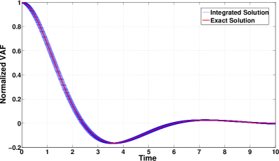
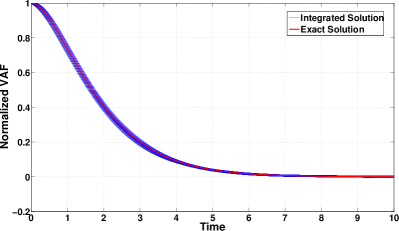
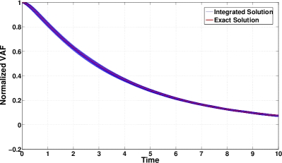
Figure 1: Normalized VAF for a single Prony series mode in the i.) underdamped ($c=1$, $\tau=1$), ii.) critically damped ($c=0.5$, $\tau=0.5$), and iii.) overdamped limits ($c=0.25$, $\tau=0.25$). A time step of $\Delta t=0.01$ is used for all runs, and error bars are drawn based upon a sample of 10,000 walkers over 10 independent runs.

To validate our integration scheme in the presence of a conservative force, we next consider GLD with an external potential. The analytic solution of the GLE with a power law memory kernel and a harmonic confining potential has been derived by other authors.Despósito and Viñales (2009) In the cited work, the GLE is solved in the Laplace domain, yielding correlation functions given in terms of a series of Mittag-Leffler functions and their derivatives. Here, we apply our integration scheme to a Prony series fit of the power law kernel and demonstrate that our results are in good agreement with the exact result over a finite time interval. The GLE that we intend to model has the form:

$$dV(t)=-\omega_{0}^{2}X(t)dt-\int\limits_{0}^{t}\frac{\gamma_{\lambda}}{\Gamma(1-\lambda)}(t-s)^{-\lambda}V(s)dsdt+M^{-1}F^{r}(t)dt,~{}~{}~{}0<\lambda<1$$ (17)

We begin by constructing a Prony series representation of the memory kernel. As it exhibits a power law decay in the Laplace domain, as well, a Prony series representation will have strong contributions from modes decaying over a continuum of time scales. To this end, rather than relying on a non-linear fitting procedure to choose values for $\tau_{k}$, we assume logarithmically spaced values from $\Delta t/10$ to $10N_{t}\Delta t$. By assuming the form of each exponential, the Prony series fit reduces to a simple linear least squares problem, that we solve using uniformly spaced data over an interval that is two decades longer than the actual simulation. In Figure 2, the Prony series fit of the memory kernel for $\lambda=0.5$ is compared to its exact value.

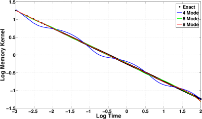
Figure 2: A Prony series fit of the power law memory kernel in Equation 17 for $\gamma_{\lambda}=1$, $\lambda=0.5$ with an increasing number of modes.

Here, the maximum relative error is $\sim 10\%$, while it is $\sim 1\%$ for $N_{k}=8$. In Figure 3, the normalized VAF computed via numerical integration of the extended GLE with a variable number of modes is shown compared to the exact result for some of the parameters utilized in an article by Despósito and Viñales.Despósito and Viñales (2009) It seems evident that the accuracy of the integrated velocity distribution improves relative to the exact velocity distribution as the number of terms in the Prony series fit increases. This is quantified in Figure 4, in which the pointwise absolute error in the integrated VAF is illustrated.

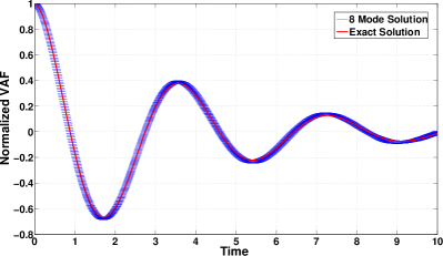
Figure 3: Comparison of numerically integrated results to the exact solution of Equation 17 for $\gamma_{\lambda}=1$, $\lambda=0.5$, and $\omega_{0}=1.4$. A time step of $\Delta t=0.01$ is used, and error bars are drawn based upon a sample of 10,000 walkers over 10 independent runs with $\Delta t=0.01$.

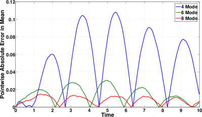
Figure 4: Pointwise absolute error in the normalized velocity autocorrelation function for the same conditions as Figure 3. Error is computed with respect to the mean of VAFs computed from 10 independent runs.

Next, we demonstrate that our implementation is robust in certain limits of the GLE - particularly the Langevin and zero coefficient limits. As our implementation is available in a public domain code with a large user base, developing a numerical method that is robust to a wide array of inputs is essential. For the zero coefficient limit we consider a harmonically confined particle experiencing a single mode Prony series memory kernel of the following form:

$$dV(t)=-\omega_{0}^{2}X(t)dt-\int\limits_{0}^{t}\frac{c}{\tau}e^{-(t-s)/\tau}V(s)dsdt+M^{-1}F^{r}(t)dt,~{}~{}~{}0<\lambda<1$$ (18)

The initial conditions on $X$ and $V$ are drawn from a thermal distribution at $T=1$. In the limit that $c\to 0$, we expect the integrated normalized VAF to approach that of a set of deterministic harmonic oscillators. The initial conditions on $X$ and $V$ are drawn from a thermal distribution at $T=1$, giving the integrated result some variance, even in the Newtonian/deterministic limit. In Figure 5, that this limit is smoothly and stably approached is illustrated.

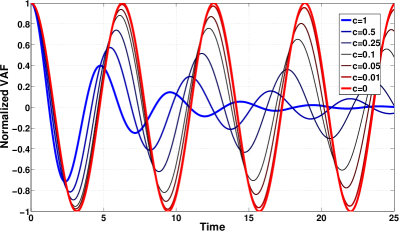
Figure 5: Illustration of the smooth/stable manner in which the proposed integrator approaches the $c=0$ (Newtonian) limit from $c=1$ for a single Prony mode with $\tau=1$. The particle is harmonically confined with $\omega_{0}=1$, and the expected period of oscillation is restored for $c=0$.

In the exact $c=0$ limit, oscillations in the VAF occur at the natural frequency of the confining potential, $\omega_{0}=1$, whereas for non-zero $c$, these oscillations are damped in proportion to $c$, as one may expect on the basis of intuition. The Langevin limit is illustrated next. To this end, we utilize the same single mode Prony series memory kernel, but remove the confining potential (i.e., $\omega_{0}=0$). We have done so to ensure that the Langevin limit yields an Ornstein-Uhlenbeck process. In Figure 6, we illustrate that this limit is also smoothly and stably approached.

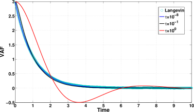
Figure 6: Illustration of the smooth/stable manner in which the proposed integrator approaches the $\tau=0$ (Langevin) limit from $\tau=1$ for a single Prony mode. The particle is subject to no conservative forces, so the resultant dynamics correspond to an Ornstein-Uhlenbeck process. The ‘exact’ Langevin limit was integrated using fix langevin in LAMMPS.

The result for the Langevin limit itself was integrated using the existing fix langevin command in LAMMPS. For $\tau=10^{0}$, the GLE yields results that differ from the Langevin limit as one might expect on the basis of the previous results. However, even for $\tau=10^{-1}$, the GLE yields results that are close to that of the Langevin limit, as the resultant numerical method retains some GLE-like behavior. However, for $\tau=10^{-8}$ and $\Delta t=0.01$, the parameter $\theta=\exp\left[-10^{6}\right]$, is below machine epsilon. As mentioned in Section II.4, this results in a method that is indistinguishable from conventional Langevin dynamics, and consequently, the integrated dynamics are indistinguishable. This result demonstrates that the method is robust, even if the user ‘accidentally’ crosses into a Langevin-like regime. We again emphasize that methods 1 and 2, considered earlier, will not stably approach this limit.

To demonstrate capability in reduced order modeling, we next invert the VAF associated with a set of trajectories generated in the presence of a conservative force, to construct a memory kernel that will reproduce the same dynamics without such a force. In other words, we seek an effective memory kernel, $\Gamma_{eff}(t)$, such that a simplified GLE of the form:

$$dV(t)=-\int\limits_{0}^{t}\Gamma_{eff}(t-s)V(s)dsdt+M^{-1}F^{r}(t)dt$$ (19)

reproduces the VAF of a GLE of the more general form given in Equation 1.

The starting point for this procedure is the observation that for Equation 19, the VAF and memory kernel have the following relationship in the Laplace domain:Mason, Gang, and Weitz (1997)

$$\langle\widetilde{V}(\sigma)V(0)\rangle=\frac{\text{k}_{B}\text{T}}{m\sigma+\widetilde{\Gamma}_{eff}(\sigma)}.$$ (20)

Here, tildes indicate that the associated time domain quantities have been Laplace transformed, with transform domain variable $\sigma$. Given $\langle\widetilde{V}(\sigma)V(0)\rangle$ for some process whose VAF we wish to reproduce via integration of Equation 19, $\widetilde{\Gamma}_{eff}(\sigma)$ can be resolved algebraically, and its time domain form can be found via an inverse Laplace transform:

$$\Gamma_{eff}(t)=\mathcal{L}^{-1}\left\{\frac{\text{k}_{B}\text{T}}{\langle\widetilde{V}(\sigma)V(0)\rangle}-m\sigma\right\}(t)$$ (21)

This effective memory kernel can then be fit to a Prony series, and Equation 19 can be integrated using the numerical method developed in this manuscript. In Figure 7, we demonstrate that we can use this inversion procedure to take the exact VAF generated by Equation 17, and compute a $\Gamma_{eff}(t)$ for Equation 19 that reproduces it:

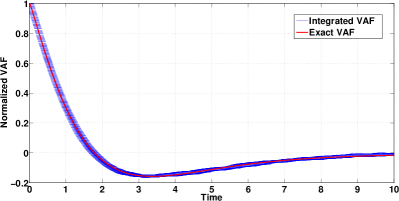
Figure 7: Illustration of the result of the kernel fitting procedure described in Section IV. Note that while the exact VAF evolves under the influence of a harmonic confining potential (Equation 17), the integrated VAF is spawned by a GLE free of any conservative forces (Equation 19). The effect of the force is included in the construction of $\Gamma_{eff}(t)$.

Here, the parameters utilized in Equation 17 were $\omega_{0}=0.5$ and $\lambda=0.9$, and the associated analytic VAF was fit to a three term Prony series. This initial fit was done to realize a simpler form of the Laplace domain VAF, which was inserted into Equation 21. The resultant $\Gamma_{eff}(t)$ was also fit to a three term Prony series. It is interesting to note that one term of this fit reduced to a conventional Langevin term (i.e., one that was proportional to $\delta(t)$ rather than $\exp\left[-t/\tau\right]$) highlighting the utility of our method’s reproduction of the Langevin limit. This Prony series representation of $\Gamma_{eff}(t)$ was used in Equation 19, which was numerically integrated to yield the integrated VAF result in Figure 7.

This result is especially interesting as it demonstrates capability for effecting a confining potential, on a finite timescale, exclusively through the GLE drag/random forces. This same fitting procedure could be used to remove inter-particle interactions, albeit with some loss of dynamical information, and will be discussed in more detail in future work.

It is important to note that while the dynamics of a confined particle are reproduced in the absence of an explicit confining force, this is only the case over the interval for which the memory kernel is reconstructed. Outside of this interval, the asymptotic behavior of the Prony series memory kernel will give rise to unbounded diffusive motion. While the expected discrepancies in the dynamics are difficult to notice in the VAF, as both the analytic and reconstructed quantities decay to zero, it is very evident in the mean-squared displacement (MSD). Here the asymptotic exponential behavior of the Prony series memory kernel necessarily leads to asymptotic diffusive motion signaled by a linear MSD. In contrast, the analytic memory kernel with the confining force will generate an MSD that remains bounded. This is illustrated in Figure 8. Here, the fit VAF is integrated to yield the MSD for the Prony series model, and compared with the exact MSD over both the interval of the fit, and beyond. This example illustrates the importance of choosing an appropriate interval for fitting memory kernels to achieve the appropriate limiting behavior in one’s dynamics.

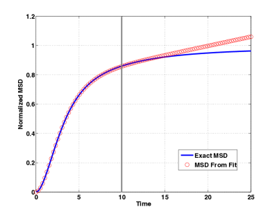
Figure 8: Comparison of the exact normalized MSD and the MSD generated from integrating the VAF fit. The exact MSD is normalized such that its asymptotic limit is 1, and the same normalization is applied to the MSD integrated from the fit. The grey line indicates the upper bound of the interval over which the VAF fit was constructed.

V Conclusions

A family of numerical integration schemes for GLD have been presented. These schemes are based upon an extended variable formulation of the GLE in which the memory kernel is rendered as a positive Prony series. In certain limits, it can be shown that a specific instance of this family of integrators exactly conserves the first and second moments of the integrated velocity distribution, and stably approaches the Langevin limit. To this end, we identify this parametrization as optimal, and have implemented it in the MD code, LAMMPS. Numerical experiments indicate that this implementation is robust for a number of canonical problems, as well as certain pathologies in the memory kernel. An exemplary application to reduced order modeling illustrates potential uses of this module for MD practitioners. Future work will further develop the VAF fitting procedure in the context of statistical inference methods, and present extensions of the numerical integrator to mixed sign and complex memory kernels.

VI Acknowledgements

The authors would like to acknowledge Jason Bernstein, Paul Crozier, John Fricks, Jeremy Lechman, Rich Lehoucq, Scott McKinley, and Steve Plimpton for numerous fruitful discussions and feedback. Sandia National Laboratories is a multi-program laboratory managed and operated by Sandia Corporation, a wholly owned subsidiary of Lockheed Martin Corporation, for the U.S. Department of Energy’s National Nuclear Security Administration under contract DE-AC04-94AL85000.

References

- Coffey, Kalmykov, and Waldron (2004) W. T. Coffey, Y. P. Kalmykov, and J. T. Waldron, The Langevin Equation With Applications to Stochastic Problems in Physics, Chemistry, and Electrical Engineering (World Scientific, 2004).
- Uhlenbeck and Ornstein (1930) G. E. Uhlenbeck and L. S. Ornstein, Phys. Rev. 36, 823 (1930).
- Kubo (1966) R. Kubo, Rep. Prog. Phys. 29, 255 (1966).
- Ermak and McCammon (1978) D. L. Ermak and J. A. McCammon, J. Chem. Phys. 69, 1352 (1978).
- Schneider and Stoll (1978) T. Schneider and E. Stoll, Phys. Rev. B 17, 1302 (1978).
- Izaguirre et al. (2001) J. A. Izaguirre, D. P. Caterello, J. M. Wozniak, and R. D. Skeel, J. Chem. Phys. 114, 2090 (2001).
- Mori (1965a) H. Mori, Prog. Theo. Phys. 33, 423 (1965a).
- Doll and Dion (1976) J. Doll and D. Dion, J. Chem. Phys. 65, 3762 (1976).
- Shugard, Tully, and Nitzan (1977) M. Shugard, J. Tully, and A. Nitzan, J. Chem. Phys. 66, 2534 (1977).
- Toxvaerd (1987) S. Toxvaerd, J. Chem. Phys. 86, 3667 (1987).
- Schweizer (1989) K. Schweizer, J. Chem. Phys. 91, 5802 (1989).
- Mason and Weitz (1995) T. G. Mason and D. A. Weitz, Phys. Rev. Lett. 74, 1250 (1995).
- Mason, Gang, and Weitz (1997) T. G. Mason, H. Gang, and D. A. Weitz, J. Opt. Soc. Am. A 14, 139 (1997).
- Fricks et al. (2009) J. Fricks, L. Yao, T. C. Elston, and M. G. Forest, SIAM J. Appl. Math. 69, 1277 (2009).
- Didier et al. (2012) G. Didier, S. A. McKinley, D. B. Hill, and J. Fricks, J. Time Series Analysis 33, 724 (2012).
- Kou and Xie (2004) S. C. Kou and X. S. Xie, Phys. Rev. Lett. 93, 180603 (2004).
- Min et al. (2005) W. Min, G. Luo, B. J. Cherayil, S. C. Kou, and X. S. Xie, Phys. Rev. Lett. 94, 198302 (2005).
- Gordon, Krishnamurthy, and Chung (2009) D. Gordon, V. Krishnamurthy, and S. Chung, J. Chem. Phys. 131, 134102 (2009).
- Ceriotti, Bussi, and Parrinello (2009) M. Ceriotti, G. Bussi, and M. Parrinello, Phys. Rev. Lett. 102, 020601 (2009).
- Ceriotti, Bussi, and Parrinello (2009) M. Ceriotti, G. Bussi, and M. Parrinello, Phys. Rev. Lett. 103, 030603 (2009).
- Ceriotti and Manolopoulos (2012) M. Ceriotti and D.E.. Manolopoulos, Phys. Rev. Lett. 109, 100604 (2012).
- Sokolov (2012) I. Sokolov, Soft Matter 8, 9043 (2012).
- Ciccotti and Ryckaert (1980) G. Ciccotti and J. Ryckaert, Mol. Phys. 40, 141 (1980).
- Berkowitz, Morgan, and McCammon (1983) M. Berkowitz, J. Morgan, and J. McCammon, J. Chem. Phys. 78, 3256 (1983).
- Guàrdia and Padró (1985) E. Guàrdia and J. Padró, J. Chem. Phys. 83, 1917 (1985).
- Straub, Borkovec, and Berne (1986) J. Straub, M. Borkovec, and B. Berne, J. Chem. Phys. 84, 1788 (1986).
- Smith and Harris (1990) D. Smith and C. Harris, J. Chem. Phys. 92, 1304 (1990).
- Nilsson and Padró (1990) L. Nilsson and J. Padró, Mol. Phys. 71, 355 (1990).
- Wan, Wang, and Shi (1998) S. Wan, C. Wang, and Y. Shi, Mol. Phys. 93, 901 (1998).
- Gordon, Krishnamurthy, and Chung (2008) D. Gordon, V. Krishnamurthy, and S. Chung, Mol. Phys. 106, 1353 (2008).
- Plimpton (1995) S. Plimpton, J. Comp. Phys. 117, 1 (1995), available at http://lammps.sandia.gov.
- in ’t Veld (2008) P. in ’t Veld, S.J. Plimpton, and G.S. Grest, Comp. Phys. Comm. 179, 320 (2008).
- Despósito and Viñales (2009) M. A. Despósito and A. D. Viñales, Phys. Rev. E 80, 021111 (2009).
- Viñales and Despósito (2006) A. D. Viñales and M. A. Despósito, Phys. Rev. E 73, 016111 (2006).
- McKinley, Yao, and Gregory (2009) S. McKinley, L. Yao, and F. Gregory, J. Rheology 53, 1487 (2009).
- Ottobre and Pavliotis (2011) M. Ottobre and G. A. Pavliotis, Nonlinearity 24, 1629 (2011).
- Wang and Skeel (2003) W. Wang and R. D. Skeel, Molecular Physics 101, 2149 (2003).
- Callen and Welton (1951) H. B. Callen and T. A. Welton, Phys. Rev 83, 34 (1951).
- Mori (1965b) H. Mori, Prog. Theo. Phys. 34, 399 (1965b).
- Kupferman (2004) R. Kupferman, J. Stat. Phys. 114, 291 (2004).
- Kloeden and Platen (1999) P. E. Kloeden and E. Platen, Numerical Solution of Stochastic Differential Equations (Springer, 1999).
- Hairer, Lubich, and Wanner (2003) E. Hairer, C. Lubich, and G. Wanner, Acta Numerica 12, 399 (2003).
- Leimkuhler and Matthews (2013) B. Leimkuhler and C. Matthews, Applied Mathematics Research eXpress 2013, 34 (2013).
- Dünweg and Paul (1991) B. Dünweg and W. Paul, International Journal of Modern Physics C 2, 817 (1991).
- Allen and Tildesley (1987) M. Allen and D. Tildesley, Computer Simulation of Liquids (Oxford University Press, 1987).
- Berne, Boon, and Rice (1966) B. J. Berne, J. P. Boon, and S. A. Rice, J. Chem. Phys. 45, 1086 (1966).