Theoretical study of solid iron nanocrystal movement inside a carbon nanotube

Abstract

We use a first-principles based kinetic Monte Carlo simulation to study the movement of a solid iron nanocrystal inside a carbon nanotube driven by the electrical current. The origin of the iron nanocrystal movement is the electromigration force. Even though the iron nanocrystal appears to be moving as a whole, we find that the core atoms of the nanocrystal is completely stationary, and only the surface atoms are moving. Movement in the contact region with the carbon nanotube is driven by electromigration forces, and the movement on the remaining surfaces is driven by diffusion. Results of our calculations also provide a simple model which can predict the center of mass speed of the iron nanocrystal over a wide range of parameters. We find both qualitative and quantitative agreement of the iron nanocrystal center of mass speed with experimental data.

I Introduction and motivation

The interior of multiwall carbon nanotubes can be filled with various metallic nanocrystals. Additionally a metallic nanocrystal will start to move inside a carbon nanotube if an electrical current is applied axially to the carbon nanotube. The speed of the nanocrystal can be tuned over many orders of magnitude, since the speed of the nanocrystal depends exponentially on the applied electrical currentBegtrup et al. (2009a). The motion of the metallic nanocrystal on the interior or exterior of the carbon nanotube has been observed previously for ironSvensson et al. (2004); Begtrup et al. (2009a, b); Loffler et al. (2011), copperGolberg et al. (2007), tungstenJin et al. (2007), indiumRegan et al. (2004), and galliumSun and Gao (2012). The movement of nanocrystals inside carbon nanotubes is interesting from the perspective of memory applicationsBegtrup et al. (2009a), as a constituted element of nanomachines, or for tunable synthesis of metal nanocrystalsCoh .

The direction of the nanocrystal movement depends on the polarity of the applied electrical current. Therefore, the movement of a nanocrystal most likely originates from electromigration forces acting on the metallic atoms such as the electron wind force. However, the precise mechanism of nanocrystal movement is not well understood. Additionally, recently it was found experimentallyCoh that an iron nanocrystal of a given diameter can move through a constriction inside a carbon nanotube of a smaller diameter while remaining an ordered solid.

We performed a series of theoretical calculations to try to understand the nature of the movement of metallic nanocrystals inside carbon nanotubes in more detail. We model a nanocrystal of iron, since this is a commonly studied nanocrystal. However we expect that the qualitative nature of movement of other metal nanocrystals will be similar to that of iron. We find that even though it appears that the iron nanocrystal is moving as a whole through the nanotube, in fact, the individual iron atoms are only moving on the surfaces of the nanocrystal. The bulk iron atoms remain stationary as long as they are in the bulk. Once the atoms that were in the bulk are exposed to the end surface, they move along the interface with the carbon nanotube towards the front surface. A somewhat related mechanism, but involving heating of iron nanocrystals and its chemical reaction with the carbon nanotube, was proposed in Ref. Loffler et al., 2011.

II Methods

Here we describe our theoretical modeling of the movement of an iron nanocrystal inside a carbon nanotube.

Although density functional theory (DFT) is a powerful technique for first-principles study of material properties, it is most commonly used to study systems with stationary positions of atoms. With the help of a molecular dynamics methodCar and Parrinello (1985), one can study dynamical properties from first-principles. However, in practice one can use first-principles molecular dynamics method only on time scales comparable to period of atomic vibrations $\sim 10^{-12}$ seconds.

In order to study movement of an iron nanocrystal inside a carbon nanotube, we need to analyze the processes on time scale close to $\sim 10^{-3}$ seconds since typical energy barriers for iron atom movement are close to 0.6 eV, while the relevant temperature is about twenty times smaller, 0.03 eV. Therefore typically an iron atom will jump across the barrier once in $\sim e^{0.6/0.03}\sim 10^{9}$ atomic vibrations, or equivalently, once every $\sim 10^{-3}$ seconds. In order to deal with these rare events, we approximate the time dynamics of this system using the kinetic Monte Carlo (kMC) method. The kinetic Monte Carlo method ignores the details of time dynamics, instead it deals only with fixed crystal sites which do or do not contain an atom at a given time. For each time step one moves an atom from one site to the next according to a rate given by energy barrier height of the move in question. Therefore, kMC simulations require only knowledge of energy barriers for iron diffusion processes.

In order to obtain reliable energy barriers for iron diffusion, we perform first principles DFT calculations of selected subsets of relevant diffusion processes in iron. We find that these barriers depend strongly on the environment of the iron atom (for example, bulk diffusion has a larger barrier than surface diffusion). Since it becomes combinatorially expensive to compute all possible iron diffusion barriers, we constructed a simple model for an estimation of any given diffusion barriers which we parametrize using our DFT calculations. We also incorporated in this model the interaction of iron atoms with the carbon nanotube. Later we will show that the qualitative nature of our results is robust under changes of parameters of this simple model.

In our calculations we do not discuss the microscopic origin of the electromigration forces on iron atoms from the current flowing through the carbon nanotube. We simply consider the electromigration force per iron atom as a parameter. Nevertheless, based on our results and experimental data from Ref. Begtrup et al., 2009a and Coh, we speculate that the origin of electromigration forces on iron is the electron wind force and not a direct force, as is the case for most metalsSorbello (1997).

II.1 Density functional theory calculation of iron diffusion

We perform a density functional theory calculation for a body-centered cubic iron diffusion in the following geometries: bulk iron diffusion and (001) and (011) surface diffusion. We consider both diffusion of surface vacancies and surface iron adatoms, and we consider the influence of a carbon overlayer on iron surface diffusion, and include both first and second neighbor hopping. Furthermore, we neglect exchange diffusion processes and only consider diffusion processes in which a single atom is displaced between initial and final configuration.

As a first step in the computation of diffusion barriers we perform full structural relaxation of initial and final configurations of the diffusion process at hand. The only exception is the relaxation of the carbon layer, since that would introduce additional numerical noise due to imperfect lattice matching between iron and carbon lattices. Therefore we only allowed rigid shifts of entire carbon layers in the direction perpendicular to the iron surface.

In a second step, we perform a nudged elastic band calculationHenkelman et al. (2000) with three configurations between initial and final configuration. For the middle of the three configurations, we use the climbing image methodHenkelman et al. (2000) to obtain a more precise value of energy barrier.

We performed density functional theory calculations using the SIESTASoler et al. (2002) computer package with a vdW-DF2 density functionalLee et al. (2010). This functional includes non-local van der Waals interaction, which are important for our calculation since ordinary GGA functionals show almost no binding between metal surfaces and a carbon layerHamada and Otani (2010). For both iron and carbon, we use norm-conserving pseudopotentials and a double-zeta polarized basis set. We use a grid cutoff energy of 440 Ry and an effective $10\times 10\times 10$ k-point grid for conventional 2-atom body-centered cubic unit cell of iron. The nudged elastic band part of the calculation was performed using an ASEBahn and Jacobsen (2002) simulation environment.

Table 1: Density functional theory computed diffusion barriers in eV for various geometries either with or without an additional carbon layer on top of the iron surface. Diffusion pathways are always considered between sites closest to the surfaces and between closest first (or second) neighbor bcc sites. For each process we also show for the diffusing atom the number of first neighbor iron atoms in initial ($Z^{i}_{\rm Fe}$) and final ($Z^{j}_{\rm Fe}$) configuration.

Type of process	Barrier (eV)	$Z^{i}_{\rm Fe}$	$Z^{j}_{\rm Fe}$
Bulk diffusion
to first neigh.	$0.72$	7	7
to second neigh.	$2.72$	8	8
Adatom diffusion
on (001) surface to second neigh.	$1.32$	4	4
on (011) surface to first neigh.	$0.36$	2	2
Vacancy diffusion
on (001) surface to first neigh.	$1.23$	7	3
on (001) surface to second neigh.	$1.17$	4	4
on (011) surface to first neigh.	$0.55$	5	5
on (011) surface to second neigh.	$1.74$	6	6
Vacancy diffusion with carbon layer
on (001) surface to first neigh.	$1.27$	7	3
on (001) surface to second neigh.	$1.15$	4	4
on (011) surface to first neigh.	$0.54$	5	5
on (011) surface to second neigh.	$1.64$	6	6

We list results for the DFT diffusion energy barrier calculations in Table 1. We find that processes with lowest energy barriers are adatom diffusion on the (011) surface (0.36 eV), vacancy diffusion on the (011) surface (0.55 eV), and first neighbor bulk diffusion (0.72 eV). All three of these processes involve diffusion between first neighbor sites. Furthermore, in all of these cases the initial and final atom configurations along the diffusion pathway are equivalent (symmetric diffusion).

Second neighbor symmetric diffusion both for bulk diffusion and (011) surface diffusion is about three to four times larger than symmetric first neighbor diffusion (2.72 eV versus 0.72 eV and 1.74 eV versus 0.55 eV). For this reason, we neglect second neighbor diffusion and focus only on first neighbor diffusion.

Furthermore, we find that asymmetric processes have different barriers than symmetric processes. For example, the energy barrier for first neighbor diffusion in bulk is 0.72 eV, while first neighbor diffusion on a (001) surface is almost twice as large, 1.23 eV. In a body-centered cubic crystal, the first neighbor diffusion on the (001) surface must occur between the top-most surface layer and the next-to-top-most surface layer. Therefore the difference in binding energy for an iron atom in these two layers explains the observed increase in first neighbor diffusion on the (001) surface.

Furthermore, we find that having a single carbon layer (graphene) next to the iron surface has negligible influence on surface diffusion of iron atoms. We computed the distance between the iron surface and the carbon layer to be 2.45 Å for a (001) surface and 3.18 Å for a (011) surface.

II.2 Model of iron diffusion

Based on theoretical calculations of iron diffusion barriers, we next describe a model which will assign an energy barrier to any diffusion process in iron.

For the diffusion of an iron atom from site $i$ to site $j$ having the same number of iron and carbon first neighbors at $i$ and $j$ site (symmetric diffusion) we assign a diffusion energy barrier $E_{i\rightarrow j}^{\rm sym}$ as,

$$E_{i\rightarrow j}^{\rm sym} =a+bZ_{\rm Fe}^{i}.$$ (1)

Here $Z_{\rm Fe}^{i}=Z_{\rm Fe}^{j}$ is the number of first neighbor iron atoms at either site $i$ (counted before an atom moves from $i$ to $j$) or site $j$ (counted after an atom moves from $i$ to $j$). We obtain values of parameters $a$ (0.21 eV) and $b$ (0.071 eV) from a fit to all first-neighbor symmetric diffusion barriers from Table 1. These three processes also have the lowest diffusion barriers and they include: adatom diffusion on the (011) surface (0.36 eV), vacancy diffusion on the (011) surface (0.55 eV), and first neighbor bulk diffusion (0.72 eV). Fitted values for these processes given by Eq. 1 are reproduced within 0.02 eV (they are respectively, 0.35 eV, 0.57 eV, and 0.71 eV).

Since we found that the presence of the carbon layer has almost no influence on symmetric diffusion processes, the energy barrier $E_{i\rightarrow j}$ in Eq. 1 does not depend on the number of carbon neighbors.

For asymmetric diffusion of an iron atom from site $i$ to site $j$, where the number of iron neighbors is different at $i$ and $j$, we assign a diffusion barrier with an additional penalty term accounting for the change in number of first neighbor atoms as,

$$E_{i\rightarrow j} =a+bZ_{\rm Fe}^{i}+\max\left(0,c\Delta Z_{\rm Fe}+d\Delta Z_{\rm C}\right).$$ (2)

$\Delta Z_{\rm Fe}$ is the difference in number of first neighbor iron atoms between sites $i$ and $j$, while $\Delta Z_{\rm C}$ is difference in the effective number of first neighbor carbon atoms. In section II.3 we describe how we assign the effective number of first neighbor carbon atoms.

The parameter $c$ quantifies the strength of the interaction between neighboring iron atoms, and it is formally similar to the exchange $J$ parameter in the Ising model. We obtained the value of parameter $c$ (0.31 eV) by comparing a DFT computed total energy for a structure with an iron vacancy in the first layer on a (001) surface to structure with iron vacancy in second layer on (001) surface. When the iron vacancy is in the first layer, the total ground state energy is lower by 1.23 eV. Since in this process exactly four iron-iron first neighbor pairs get broken ($Z^{i}_{\rm Fe}-Z^{j}_{\rm Fe}=7-3=4$), we obtain $c=1.23/4=0.31$ eV. We decided not to fit first-neighbor diffusion process on the (001) surface directly to Eq. 2, since in our DFT calculations we find that this process does not have an energy saddle point, instead the energy is monotonically increasing while going from the initial to the final configuration. Instead, we find it more important to obtain a more reliable value of the iron-iron interaction strength. We obtain a similar value of parameter $c$ by considering the displacement of the iron vacancy between first and second layers of the (011) surface (0.33 eV) where only two iron-iron first neighbor pairs get broken. Somewhat larger values of parameter $c$ are obtained from surface formation energy of the (001) surface (0.37 eV) and the (011) surface (0.50 eV). In section III.1.5 we show the robustness of our results to changes to value of this and other model parameters.

Parameter $d$ quantifies the strength of the iron-carbon interaction. We obtained a value for parameter $d$ (0.14 eV) by comparing the DFT computed energy of an iron surface terminated with a carbon layer (graphene) to a DFT energy of clean iron surface and a carbon layer in vacuum. The value for the parameter $d$ for a (001) iron surface (0.13 eV) is somewhat smaller than on a (011) iron surface (0.15 eV), which is why we use their arithmetic average in the calculation.

In our model, we neglect diffusion of iron atoms to second nearest neighbor since those processes have higher diffusion barriers (see Table 1). Furthermore, our DFT calculations show that the energy required to remove single iron atom from bulk or surface to the vacuum is much underestimated by the penalty term $c\Delta Z_{\rm Fe}$ from Eq. 2. For such process one would need to use an effective value of $c$ to be 0.90, 1.05, or 1.46 eV (for an atom removal from bulk, (011), and (011) surfaces respectively) which is three to five times larger than the value of $c$ we obtained earlier. For this reason, we have decided to simply neglect processes in which an atom moves to site $j$ which does not have any iron atoms in first neighbor sites ($Z^{j}_{\rm Fe}=0$).

II.3 Kinetic Monte Carlo simulation

Given the model from Sec. II.2 to describe the diffusion process in iron, we can proceed to do a kinetic Monte Carlo simulation of an iron nanocrystal movement inside a carbon nanotube.

We first define a fixed set of atomic sites along which iron atoms can move. We start with an infinite arrangement of body-centered cubic sites with an iron lattice constant $a=0.29$ nm. Next, we construct a cylinder with radius $r_{\textrm{cyl}}$ about an order of magnitude larger than $a$ immersed in this infinite arrangement of body-centered cubic lattice sites. We ignore all iron sites outside of this cylinder and consider only sites inside the cylinder, to simulate an iron nanocrystal contained inside carbon nanotube. We take the orientation of the cylinder axis to point along the crystal [100] direction as found experimentallyBegtrup et al. (2009b). At the beginning of the simulation (time $t=0$), we occupy certain number of such sites within the tube, while all other sites inside the cylinder (carbon nanotube) are initially empty. For simplicity we always start from a configuration in which the occupied sites are taken in a certain range of heights $[z_{\rm min},z_{\rm max}]$ along the cylinder axis.

Starting from an initial arrangement of iron atoms we compile a list of all possible moves that iron atoms can make. Our DFT calculation has shown that it is sufficient to consider only moves of iron atoms to empty first nearest neighbor sites. To each such move from the list (between sites $i$ and $j$) we assign a rate $\rho_{i\rightarrow j}$,

$$\rho_{i\rightarrow j}=\rho_{0}\exp\left[-\frac{E_{i\rightarrow j}}{kT}+\frac{\frac{1}{2}({\bm{r}}_{j}-{\bm{r}}_{i})\cdot{\bm{F}}_{\rm em}}{kT}\right].$$ (3)

Here $\rho_{0}$ is constant commonly used in kMC modeling ($\rho_{0}=10^{12}$ s^-1) corresponding to the inverse of a typical phonon frequency, $k$ is Boltzmann constant, $T$ is the simulation temperature, and $E_{i\rightarrow j}$ is the energy barrier height as computed from a first-principles based model given in Eq. 2.

Since an iron nanocrystal and a carbon layer have incommensurate lattices, the assignment of the number of carbon neighbors to a given iron site becomes difficult. Therefore we employ the following simple scheme to assign the number of first neighbor carbon atoms. For each iron site on the boundary of the nanocrystal, we simply count the number of first neighbor iron-iron pairs broken by the cylindrical cut and we assign that number to be the effective number of carbon bonds.

Finally, ${\bm{r}}_{i}$ and ${\bm{r}}_{j}$ in Eq. 3 are Cartesian coordinate vectors for atomic sites $i$ and $j$, while ${\bm{F}}_{\rm em}$ is the electromigration force acting on an iron atom, originating from the current in the carbon nanotube. Assuming that the energy barrier maximum between sites $i$ and $j$ occurs halfway in between, the factor $\frac{1}{2}({\bm{r}}_{j}-{\bm{r}}_{i})\cdot{\bm{F}}_{\rm em}$ appearing in Eq. 3 accounts for increase in diffusion rate $\rho_{i\rightarrow j}$ along the direction of the electromigration force. Similarly, this factor reduces diffusion rate $\rho_{i\rightarrow j}$ in the direction opposite to the electromigration force.

We assume that the force ${\bm{F}}_{\rm em}$ is non-zero only if either site $i$ or $j$ is adjacent to the nanotube (i.e. either site $i$ or site $j$ has non-zero number of effective carbon neighbors), and we test robustness of this assumption in section III.1.5. Furthermore, we take the vector ${\bm{F}}_{\rm em}$ to point in the direction of the cylinder (nanotube) axis, along the direction of the current. The magnitude of the vector ${\bm{F}}_{\rm em}$ is then taken as a parameter of the simulation. In Sec. III.1.4 we relate force ${\bm{F}}_{\rm em}$ to the electrical current density $j$.

Now that we have assigned the rate $r_{i\rightarrow j}$ to each possible atomic move $i\rightarrow j$ in the initial configuration, we proceed by performing atomic steps. We choose which step to perform based on a standard kMC probabilistic modelBortz et al. (1975); Voter (2007) which chooses at random one of the steps according to the rate given by Eq. 3. Once the move has been performed the simulation time is updated from $t=0$ to $t=\Delta$ according to the rates given by Eq. 3. Since performing this atomic step has altered the atom configuration, we need to update the list of all possible moves and update the rates assigned to the moves. With an updated list of moves and their rates, we repeat this process until we reach the desired number of simulation steps, or the desired simulation time $t$. In order to speed up the kMC simulation, we also employ the binary tree algorithmBlue et al. (1995).

III Results and discussion

In this section we will present results of our kinetic Monte Carlo simulation.

III.1 Character of movement in constant cross-section area carbon nanotube

We find that for a wide range of parameters, the iron nanocrystal can move through a carbon nanotube under the application of an external electromigration force. Figure 1 shows the dependence of the nanocrystal center of mass speed on the magnitude of the electromigration force per atom $F_{\rm em}=|{\bm{F}}_{\rm em}|$ for fixed simulation temperature, nanocrystal area, and length. It is clear that the speed depends non-linearly on the external force just as in the experimentsBegtrup et al. (2009a); Loffler et al. (2011). We postpone the analysis of the center of mass speed dependence on force, temperature, area, and length to sections III.1.1,III.1.2, and III.1.3. Here we first focus on the nature of iron nanocrystal movement in the nanotube.

It is easier for demonstration purposes to describe the nanocrystal motion for temperatures somewhat higher than those found in experimentBegtrup et al. (2009a). Therefore we defer analysis of our model calculation in experimental range of temperatures to Sec. III.1.4.

Figure 2 shows the cross-section along cylinder axis of the iron nanocrystal and carbon nanotube. Four regions of the iron nanocrystal are indicated. Regions A, B, and C consist of atoms on the boundary of the nanocrystal, while atoms in region D are in the bulk (core) of the nanocrystal. Furthermore, the circular regions A and C are on opposite sides (caps) of the nanocrystal, while the cylindrical shell B is in contact with the carbon nanotube. In the following discussion the assignment of regions A, B, C, and D is assumed to be stationary, i.e. atoms can move from one region to another, but the region assignment relative to nanocrystal remains the same. For definiteness we assume that the electromigration force is pointing to the right in Fig. 2.

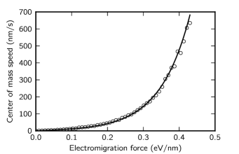
Figure 1: Computed iron nanocrystal center of mass speed as a function of electromigration force $F_{\rm em}$. Simulation temperature is 700 K, somewhat larger than in the experimentBegtrup et al. (2009a), iron nanocrystal radius is $r_{\textrm{cyl}}$=1.05 nm, and the length is $l=4.31$ nm. Line is a fit to functional form as in Eq. 4.

Our kMC simulation shows that atoms in region D are stationary, as long as they remain in region D. Atoms in region B under the influence of the electromigration force get pushed towards region C, where they diffuse evenly along the cylinder cap. Vacancies created in region B create a concentration gradient which by diffusion attracts atoms from region A to region B.

We now focus on the movement of a single atom that starts out in region A. Under the influence of the diffusion force created by vacancies in region B, this atom will eventually reach region B. Once in region B under the influence of the electromigration force it will move toward region C. Once it reaches region C, it will distribute there with near uniform probability, again due to diffusion forces. After more and more atoms get extracted from region A into region C, this particular atom will eventually get covered by enough layers of new atoms so that it will effectively become part of region D. Once in region D, this atom remains stationary! Once all remaining atoms are removed from region A and added to region C, this atom will become part of region A and the entire process repeats. Therefore, schematically the pattern of movement of individual iron atom can be described as,

$$A\xlongrightarrow[\textrm{diffusion}]{}B\xlongrightarrow[F_{\rm em}]{}B\xlongrightarrow[\textrm{diffusion}]{}C\xlongrightarrow[\textrm{wait}]{}D\xlongrightarrow[\textrm{wait}]{}A.$$

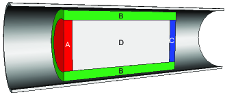
Figure 2: Cross-section of iron nanocrystal inside carbon nanotube. Four regions of the nanocrystal are indicated (A, B, C, and D) see main text for details. For definiteness, the direction of the electromigration force is assumed to be to the right in this figure.

Figures 3 and 4 show eight snapshots of the single kinetic Monte Carlo simulation of the iron nanocrystal movement inside a carbon nanotube with constant cross-section. The first snapshot ($t=0$ ms) corresponds to the initial configuration, the second snapshot follows after $t=10$ ms, while the remaining six snapshots all follow in intervals of 30 ms from the initial configuration. Figure 3 shows projection of atom coordinates (gray spheres) onto two-dimensional plane parallel to the cylinder (nanotube) axis. From this figure we can see that the carbon nanotube in this particular configuration moves by its one length in roughly 180 ms.

Figure 3: Two dimensional projection of three dimensional iron atom positions at eight different snapshots in the kinetic Monte Carlo simulation. Various intensities of greyness correspond to rows containing more (darker gray) or less (brighter gray) iron atoms. The simulation temperature is 700 K, somewhat larger than in the experimentBegtrup et al. (2009a), iron nanocrystal radius is $r_{\textrm{cyl}}$=1.11 nm, and the length is $l=4.31$ nm. The electromigration force magnitude is $F_{\rm em}=0.28$ eV/nm.

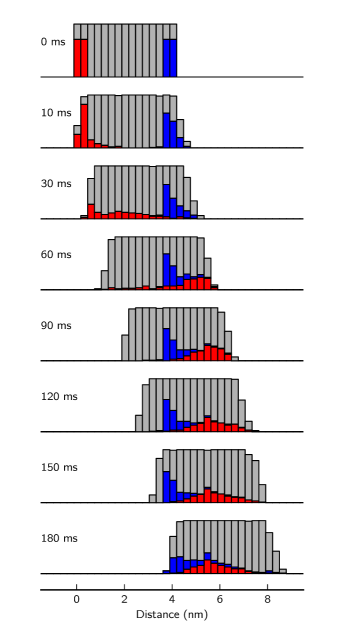
Figure 4: Results from the same kinetic Monte Carlo simulation as in Fig. 3 in the form of a histogram indicating the number of iron atoms within each bin with length of one lattice constant($a=0.29$ nm). The number of atoms initially in region A (B) are colored red (blue) and their positions are tracked during the simulation. Vertical position of the bars in the histograms are arbitrary, only the height of each individual bar (gray, red, or blue) is to be interpreted as the number of atoms within that bin.

Figure 4 shows, for the same kinetic Monte Carlo run as in Fig. 3, the distribution of atom occupation in the form of a histogram. Each bin in the histogram has a length of one lattice constant ($a=0.29$ nm), and its height represents the number of iron atoms within that region of the nanocrystal. Additionally, Fig. 4 indicates, in red and blue, the number of atoms that are in the initial configuration ($t=0$ ms) in regions A and C respectively (vertical position of gray, red, and blue regions is meaningless). In subsequent snapshots, these atoms move from one region to another, as discussed previously. For example, we find that atoms which at $t=0$ ms are in region A (red) by time $t=30$ ms are almost entirely in region B. By $t=90$ ms these atoms are distributed along regions C and D, while at $t=180$ ms they are entirely in region D. On the other hand, atoms initially ($t=0$ ms) in region C (blue) are in region D by $t=30$ ms and remain stationary in region D until entering region A at $t=180$ ms.

Finally, Fig. 5 shows the computed flow of atoms in the nanocrystal as a function of their radial coordinate and the coordinate along the cylinder axis. For each step in the kinetic Monte Carlo simulation we recorded the initial atomic coordinate (${\bm{r}}_{i}$) in the nanocrystal center-of-mass reference frame and direction of atomic step (${\bm{r}}_{j}-{\bm{r}}_{i}$). For a given coordinate ${\bm{r}}_{i}$ averaging the directions of performed atomic steps over all kinetic Monte Carlo steps involving site ${\bm{r}}_{i}$ gives us a flow vector ${\bm{f}}_{i}\sim\sum({\bm{r}}_{j}-{\bm{r}}_{i})$ at that point. Darker regions in Fig. 5 indicate points with larger magnitude of flow vector ${\bm{f}}_{i}$ in logarithmic scale. Arrows in Fig. 5 indicate the direction of flow vector ${\bm{f}}_{i}$. We have neglected azimuthal components of ${\bm{f}}_{i}$. Additionally, Fig. 5 shows flow vectors summed over azimuthal component of initial coordinate ${\bm{r}}_{i}$.

We conclude from Fig. 5 once again that atoms are moving only on the surfaces (regions A, B, and C) while they remain stationary in the bulk (region D). Furthermore, from here we infer that atomic flow in regions A and C (caps) is about 10 to 100 times larger than flow in region B (this difference is somewhat obscured by the logarithmic scale in Fig. 5).

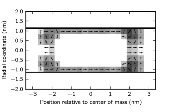
Figure 5: Flow of iron atoms in the iron nanocrystal during its movement through the nanotube. See main text for a more detailed description. Larger flow magnitude is indicated with darker shade of gray, on a logarithmic scale. Direction of flow is shown with arrows (regardless of magnitude, all arrows have the same length). For clarity all flow information is duplicated from positive radial coordinates to the negative coordinates. The simulation temperature in this calculation is 600 K, somewhat larger than in the experimentBegtrup et al. (2009a), iron nanocrystal radius is $r_{\textrm{cyl}}$=1.11 nm, and the length is $l=4.31$ nm. The electromigration force magnitude is $F_{\rm em}=0.28$ eV/nm.

III.1.1 Dependence on nanocrystal length

In our kMC simulations we varied nanocrystal lengths from $l=3$ nm up to $l=40$ nm (in temperature ranges from 500 to 900 K). We find that the center of mass speed is nearly independent of the nanocrystal length. This means that movement of iron atoms near the carbon nanotube (region B) is much more efficient than the diffusion in regions A and C. In other words, it takes an iron atom long time to go from region A to B (or vacancy to go from B to C), but once iron atom reaches region B it proceeds quickly to region C on the other side of the nanocrystal.

III.1.2 Dependence on temperature and electromigration force

We find a very strong dependence of the nanocrystal center of mass speed on the temperature and electromigration force. Circular symbols in Fig. 6 show kinetic Monte Carlo results for the iron nanocrystal center of mass speed on a logarithmic scale for varying temperature and electromigration force. (Similarly, Fig. 1 shows in linear scale speed for a single temperature.) Nanocrystal cross-sectional area and length in this calculation are kept constant.

When the electromigration force on iron atoms becomes too large, we find that the iron nanocrystal movement becomes unstable and it can breakup into smaller pieces. Occurrence of such instability in the model also depends on the thickness of region in which iron atoms experience electromigration force, and we discuss this dependence in more detail in Sec. III.1.5. Some experimental evidence for this kind of behavior has been seen in Ref. Svensson et al., 2004.

Kinetic Monte Carlo results shown in Fig. 6 clearly show that motion of iron nanocrystal is temperature activated, which motivated us to model its movement with that of an effective single particle in an external potential. In appendix A we derived an expression for the speed of one particle in periodic external potential (barrier height $B$ and period $L$) under the influence of constant external force $F$, and in contact with a thermal bath at temperature $T$. Using this expression we can now try to fit our kinetic Monte Carlo results for center of mass speed to the following functional form,

$$v=\tilde{v}\exp\left(-\frac{\tilde{B}}{kT}\right)\sinh\left(\frac{\frac{1}{2}\tilde{L}F}{kT}\right).$$ (4)

Here $\tilde{v}$, $\tilde{B}$, and $\tilde{L}$ are fitting parameters which correspond respectively to the velocity prefactor, barrier height and period of external potential for this single effective particle. We set force $F$ to equal electromigration force experienced by a single iron atom in the simulation, $F_{\rm em}$.

Lines in Fig. 6 show the fit of the kinetic Monte Carlo simulation results to the functional form given by Eq. 4. One can see that this functional form reproduces quite well simulated results. Fitted values of for velocity prefactor $\tilde{v}$, effective barrier height $\tilde{B}$, and effective period $\tilde{L}$ are,

$$\tilde{v}=3.3\textrm{~{}m/s,}\quad\tilde{B}=1.2\textrm{~{}eV,}\quad\tilde{L}=1.4\textrm{~{}nm.}$$ (5)

III.1.3 Dependence on nanocrystal cross-section area

Finally, we analyze the dependence of iron nanocrystal center of mass speed on the nanocrystal cross-section area. The number of atoms that need to travel from region A to region C in order for the crystal to move a certain fixed length is proportional to nanocrystal cross-section area $\sim r_{\textrm{cyl}}^{2}$. However, with increasing cross-sectional area the number of pathways to travel through region B is also increasing, but only as $\sim r_{\textrm{cyl}}^{1}$. Naively, one would therefore expect that center of mass speed of an iron nanocrystal will be proportional to $\sim r_{\textrm{cyl}}^{-1}$. However, our calculations find that there is lot of variations on top of overall trend of decreasing center of mass speed with radius $r_{\textrm{cyl}}$. The reason for this discrepancy we find in the following. Nature of diffusion pathways in region B of iron nanocrystal will depend strongly on the details of the cylindrical boundary of the iron nanocrystal. For example, we find that for some specific values of nanocrystal radius $r_{\textrm{cyl}}$ one can have in region B precisely two rows of iron atoms on top of iron (011) surfaces. Our model from Eq. 2 predicts that there is very small diffusion barrier for movement along these two rows of atoms (since $Z^{i}_{\rm Fe}=Z^{j}_{\rm Fe}=3$) which means that movement along region B (and possibly into or out of region B) is greatly enhanced.

Repeating the fit to the effective particle model from Eq. 4 for nanocrystals with varying cross-sectional area we find that fitting parameters appearing in exponential and sinus hyperbolic functions: $\tilde{B}$ and $\tilde{L}$ are almost unaffected. Only parameter which seems to depend on cross-section area is velocity prefactor $\tilde{v}$, which is of smaller importance. For example, when comparing our results to experiment in Sec. III.1.4 precise value of $\tilde{v}$ will be of almost negligible importance as compared to values of $\tilde{B}$ and $\tilde{L}$ appearing inside exponential and sinus hyperbolic functions in fitting function, Eq. 4.

More specifically, we performed calculations for five different nanocrystal radii $r_{\textrm{cyl}}$ ranging from $1.05$ nm to $1.73$ nm, corresponding to cross-sectional area from 3.46 nm² to 9.40 nm². Among these five calculations we find that largest fitted value of parameter $\tilde{v}$ is about three times larger than for the case with smallest value of $\tilde{v}$. On the other hand, parameters $\tilde{B}$ and $\tilde{L}$ are varying only about 10%.

III.1.4 Comparison with experiment

In Ref. Begtrup et al., 2009a the speed of an iron nanocrystal was measured as a function of an applied external voltage $V$ and current $I$ (red square symbols in Fig. 6). On the other hand, in our kinetic Monte Carlo simulation we compute the speed of an iron nanocrystal as a function of electromigration force $F_{\rm em}$ (black circles in Fig. 6). In order to relate $F_{\rm em}$ to $I$ we first assume that the electromigration force $F_{\rm em}$ is linearly proportional to the current density $j$,

$$F_{\rm em}=Kj,$$ (6)

and we later obtain the parameter $K$ by fitting to the experiment. (The linear dependence of $F_{\rm em}$ on $j$ as in Eq. 6 is consistent with an electron wind force mechanism as discussed in Refs. Sorbello, 1997; Dekker and Lodder, 1998.)

We crudely estimate the current density $j$ in the iron nanocrystal by making the following set of assumptions. First, we assume a constant current density profile perpendicular to the carbon nanotube axis, both in the iron nanocrystal and in the carbon nanotube. Second, we assume that the conductivity of the iron nanocrystal equals that of the bulk iron. Both of these assumptions likely underestimate the current density $j$ (and therefore overestimate $K$). Nevertheless, under these assumptions, current density $j$ flowing through the iron nanocrystal is given as,

$$j=\frac{I}{A_{\rm tube}}\left(\frac{\rho_{\rm iron}}{\rho_{\rm tube}}+\frac{A_{\rm iron}}{A_{\rm tube}}\right)^{-1}.$$ (7)

Here, $A_{\rm tube}$ and $A_{\rm iron}$ are cross-sectional area of carbon nanotube and iron nanocrystal respectively. We estimate $A_{\rm tube}$ and $A_{\rm iron}$ from inner and outer diameters of the carbon nanotube used in Ref. Begtrup et al., 2009a ($5-7$ nm and $35$ nm respectively). For the resistivity of iron $\rho_{\rm iron}$, we use $8.6\cdot 10^{-8}$ $\Omega$ m, while the resistivity of the carbon nanotube $\rho_{\rm tube}$ we can compute from the length of the tube (2 $\mu$m), $A_{\rm tube}$, $V$, and $I$. This procedure gives us $\rho_{\rm tube}\sim 2.6\cdot 10^{-6}$ $\Omega$ m, close to the bulk resistivity of graphite.

We obtain good agreement with experimental measurementsBegtrup et al. (2009a) of the iron nanocrystal center of mass speed using $K=0.18$ eV nm/$\mu$A and temperature $T=350$ K (compare dashed red line and red symbols in Fig. 6). However, we expect that there is a large uncertainty in value of parameter $K$ due to our crude estimate of current density $j$. We are unaware of any other theoretical or experimental estimates of electromigration force coefficient $K$ in iron. Additionally, the value of the parameter $K$ varies a lot across the periodic tableDekker and Lodder (1998) both in magnitude and sign. Furthermore, the value of the parameter $K$ is very sensitive to the structural parameters. For example, it can vary a great deal between fcc and bcc phases of the materialDekker and Lodder (1998). Interestingly enough, the largest value of the parameter $K$ among all cases studied in Ref. Dekker and Lodder, 1998 is that of an iron impurity electromigrating in aluminum ($K=0.01$ eV nm/$\mu$A), which is within an order of magnitude of our estimated value of $K$.

Experiments in Ref. Begtrup et al., 2009a have been performed at room temperature, but the actual temperature on the carbon nanotube has not been measured directly. Independent estimates, based on Joule heating and thermal conductivity of the Si₃N₄ substrate, give an estimated temperature of $\approx 440$ K, consistent with our fitted value. A similar value is obtained by scaling the Joule heating power to that used in Ref. Begtrup et al., 2007 where temperature of the carbon nanotube has been directly measured.

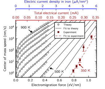
Figure 6: Dependence of iron nanocrystal center of mass speed on electromigration force (black) and total electrical current $I$ (red). Kinetic Monte Carlo simulation (black circles) was done for temperatures from 500 K to 900 K in steps of 50 K, iron nanocrystal radius for all calculations equals $r_{\textrm{cyl}}$=1.05 nm, while length is $l=4.31$ nm. A fit to model from Eq. 4 with parameters given in Eq. 5 is shown with black lines for temperatures from 350 K to 900 K in steps of 50 K. Experimental data from Ref. Begtrup et al., 2009a is shown with red squares, and fit to model from Eq. 4 to experimental data is shown with red dashed line (temperature used in fit is $350$ K, consistent with an independent experimental estimate). Relationship between electromigration force (bottom axis, black) and estimated current density $j$ through the iron nanocrystal (topmost axis, blue) is given by Eq. 6 as discussed in the text.

III.1.5 Robustness of results on model parameters

Now we will discuss robustness of our results on changes in model parameters. There are four parameters ($a$, $b$, $c$, and $d$) in Eq. 2 which have all been fitted to first-principles DFT calculation. Additionally we assumed that the electromigration force ${\bm{F}}_{\rm em}$ influences only iron steps when either initial site $i$, or final site $j$ are immediately next to the carbon nanotube.

Let us start by testing robustness of our results on four parameters from Eq. 2. We performed series of calculations in which we either increased or decreased by 15% each of these four parameters separately. We find in all eight calculations that qualitative character of iron nanocrystal movement remains unchanged. Additionally, dependence on temperature and electromigration force remains qualitatively the same as in Eq. 4. Quantitatively, we find small changes in the fitting parameters $\tilde{v}$, $\tilde{B}$, and $\tilde{L}$. The resulting iron nanocrystal center of mass speed is more sensitive to parameters $b$ and $c$ than to $a$ and $d$.

Additionally, we tried removing the dependence of diffusion energy barrier height on initial number of first neighbor iron atoms $Z_{\rm Fe}^{i}$. Therefore we set parameter $b$ to zero and vary value of parameter $a$. We again find qualitatively the same dependence of center of mass speed as in Eq. 4. We changed the value of the parameter $a$ from 0.4 to 0.7 eV and the main quantitative difference we find is that effective period $\tilde{L}$ is about two times smaller then using original values of $a$, $b$, $c$, and $d$ parameters.

Another robustness test we performed is to increase region in which iron atoms feel influence of the electromigration force ${\bm{F}}_{\rm em}$. Instead of just considering atoms which are in contact with carbon atoms, we redid calculation in which this region was increased so as to include iron atoms up to 0.4 nm away from the carbon nanotube. Also, as an extreme case, we redid calculation where electromigration force ${\bm{F}}_{\rm em}$ was acting on all iron atoms. We find that with different regions in which the force ${\bm{F}}_{\rm em}$ is acting on the iron nanocrystal center-of-mass is almost unaffected.

Nevertheless, we find that with increasing region in which force ${\bm{F}}_{\rm em}$ is acting, iron nanocrystal starts to breakup at smaller and smaller forces. When only first layer of iron atoms is experiencing electromigration force, nanocrystal starts to break when force $|{\bm{F}}_{\rm em}|$ is larger than 0.5 eV/nm (other parameters are as in data from Fig. 1). When iron atoms up to 0.4 nm away from the nanotube are experiencing electromigration force, nanocrystal breaks up for forces above 0.25 eV/nm. Finally, when all iron atoms are experiencing electromigration force, breaking occurs already above 0.15 eV/nm.

III.2 Movement through a constriction

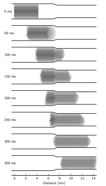
Figure 7: Two dimensional projection of three dimensional iron atom positions at eight different snapshots in the kinetic Monte Carlo simulation, as in Fig. 3. Various intensity of greyness correspond to rows containing more (darker gray) or less (brighter gray) iron atoms. The simulation temperature is 700 K, somewhat larger than in the experimentCoh , iron nanocrystal radius in the region on the left is $r_{\textrm{cyl}}$=1.35 nm, and on the right is $r_{\textrm{cyl}}$=1.11 nm (as in Fig. 3). Therefore, cross-section area on the left is about 50% larger than on the right. Length of iron crystal at $t=0$ ms is $l=4.31$ nm. The electromigration force magnitude is $F_{\rm em}=0.28$ eV/nm.

Now we will describe movement of iron nanocrystal through a tube with a varying cross-section. At first, it seems surprising that solid piece of iron nanocrystal could move through constrictions in nanotube with cross-section smaller than nanocrystal cross-section. However, taking into account the character of the iron nanocrystal movement we discuss in Sec. III.1, it becomes clearer why this is possible. Iron atoms in region D remain stationary and therefore do not need to move through a constriction directly. On the other hand, when iron atoms move from region B into region C, they adapt to tube with smaller cross-section. Movement of iron nanocrystal through a constriction in the carbon nanotube has been experimentally demonstrated in Ref. Coh, .

Figure 7 shows kinetic Monte Carlo simulation results of a movement of iron nanocrystal through a tube with area 5.7 nm² that gets shrunk to 3.9 nm². One can see that between moment $t=50$ ms and $t=300$ ms iron nanocrystal was able to move through a constriction. We find the same behavior for other ratio of nanotube cross-sections.

IV Conclusion

Our first-principles based on kinetic Monte Carlo simulations of iron nanocrystal inside carbon nanotube show the nature of movement of iron nanocrystal. We find that the iron nanocrystal does not move as a whole but instead atoms are moving only on the surfaces, from one end of crystal to the other. See Sec. III.1 for more detail. Consistent with this observation, we also find that an iron nanocrystal is able to move through a constriction in the carbon nanotube that has larger diameter than the nanocrystal.

Somewhat surprisingly we find theoretically that an iron nanocrystal center of mass speed does not depend on the length of the nanocrystal. We attribute this to the fact that individual iron atom moves through region B quite fast, compared to time spent in region A, or C. Furthermore, we find that movement of entire nanocrystal can be modeled quite well as thermally activated motion of single particle in tilted periodic potential with period of 1.4 nm, and barrier height 1.2 eV, regardless of carbon nanotube area, length, temperature, or electromigration force. In future, it would be interesting to measure experimentally dependencies of center of mass speed on nanocrystal length, area, and temperature. So far, only dependence on external current has been established, for fixed length, area, and temperature.

In our model we assumed that only iron atoms next to the carbon nanotube are experiencing electromigration forces. Nevertheless, even if we allow a larger region of iron atoms to experience electromigration force (or even entire iron nanocrystal) we still find that iron nanocrystal can move through the carbon nanotube. However, as this region gets larger and larger, movement of iron nanocrystal becomes more and more unstable.

Comparing the experimentally measured speed of an iron nanocrystal with our model calculation we estimate that temperature of iron nanocrystal is not much larger than room temperature ($\sim 350$ K) which is in agreement with crude estimates from Joule heating. Furthermore, we find that relationship between current density through iron nanocrystal and force on individual iron atoms is given by constant of proportionality $K=0.18~{}\textrm{eV nm}/\mu\textrm{A}$.

Appendix A Diffusion in one-dimensional periodic potential

Diffusion in a one-dimensional periodic potential $U(x+L)=U(x)$ under application of an external force $F$ can be modeled by the following equation of motion,

$$\eta\frac{dx}{dt}=F-\frac{dU}{dx}+\sqrt{2\eta kT}\xi(t).$$ (8)

Here $\eta$ is friction coefficient, and $x(t)$ is position of particle at time $t$. The stochastic force on the particle due to thermal fluctuations at temperature $T$ is modeled by a random variable $\xi(t)$ with zero mean value, $\left\langle\xi(t)\right\rangle=0$ and a Dirac delta correlation, $\left\langle\xi(t)\xi(t^{\prime})\right\rangle=\delta(t-t^{\prime})$. The analytic expression for the average velocity of the particle governed by such equation is given asRisken (1996),

$$v=\frac{LkT}{\eta}\frac{1-\exp\left(-\frac{LF}{kT}\right)}{\int_{0}^{L}\int_{0}^{L}\exp\frac{U(x)-U(x-x^{\prime})-Fx^{\prime}}{kT}dxdx^{\prime}}.$$ (9)

For a sawtooth potential ($U(x)=x\frac{2B}{L}$ for $0<x<L/2$ and $U(x)=2B-x\frac{2B}{L}$ for $L/2<x<L$) with period $L$ and barrier height $B$ one can show that in the limit of $kT\ll B$ and $\frac{1}{2}FL<B$ velocity of particle is given as,

$$v\approx\frac{2B^{2}}{\eta LkT}\exp\left(-\frac{B}{kT}\right)\sinh\left(\frac{\frac{1}{2}LF}{kT}\right).$$ (10)

References

- Begtrup et al. (2009a) G. E. Begtrup, W. Gannett, T. D. Yuzvinsky, V. H. Crespi, and A. Zettl, Nano Letters 9, 1835 (2009a).
- Svensson et al. (2004) K. Svensson, H. Olin, and E. Olsson, Phys. Rev. Lett. 93, 145901 (2004).
- Begtrup et al. (2009b) G. E. Begtrup, W. Gannett, J. C. Meyer, T. D. Yuzvinsky, E. Ertekin, J. C. Grossman, and A. Zettl, Phys. Rev. B 79, 205409 (2009b).
- Loffler et al. (2011) M. Loffler, U. Weissker, T. Muhl, T. Gemming, J. Eckert, and B. Buchner, Advanced Materials 23, 541 (2011).
- Golberg et al. (2007) D. Golberg, P. Costa, M. Mitome, S. Hampel, D. Haase, C. Mueller, A. Leonhardt, and Y. Bando, Advanced Materials 19, 1937 (2007).
- Jin et al. (2007) C. Jin, K. Suenaga, and S. Iijima, Nat. Nano. 3, 17 (2007).
- Regan et al. (2004) B. C. Regan, S. Aloni, R. O. Ritchie, U. Dahmen, and A. Zettl, Nature 428, 924 (2004).
- Sun and Gao (2012) M. Sun and Y. Gao, Nanotechnology 23, 065704 (2012).
- (9) S.C., W.G., A.Z., S.G.L., M.L.C., PRL 2013.
- Car and Parrinello (1985) R. Car and M. Parrinello, Phys. Rev. Lett. 55, 2471 (1985).
- Sorbello (1997) R. S. Sorbello, in Theory of Electromigration, Solid State Physics, Vol. 51, edited by H. Ehrenreich and F. Spaepen (Academic Press, 1997) pp. 159 – 231.
- Henkelman et al. (2000) G. Henkelman, B. P. Uberuaga, and H. Jónsson, The Journal of Chemical Physics 113, 9901 (2000).
- Soler et al. (2002) J. M. Soler, E. Artacho, J. D. Gale, A. Garcia, J. Junquera, P. Ordejon, and D. Sanchez-Portal, Journal of Physics: Condensed Matter 14, 2745 (2002).
- Lee et al. (2010) K. Lee, E. D. Murray, L. Kong, B. I. Lundqvist, and D. C. Langreth, Phys. Rev. B 82, 081101 (2010).
- Hamada and Otani (2010) I. Hamada and M. Otani, Phys. Rev. B 82, 153412 (2010).
- Bahn and Jacobsen (2002) S. R. Bahn and K. W. Jacobsen, Comput. Sci. Eng. 4, 56 (2002).
- Bortz et al. (1975) A. Bortz, M. Kalos, and J. Lebowitz, Journal of Computational Physics 17, 10 (1975).
- Voter (2007) A. Voter, in Radiation Effects in Solids, NATO Science Series, Vol. 235, edited by K. Sickafus, E. Kotomin, and B. Uberuaga (Springer Netherlands, 2007) pp. 1–23.
- Blue et al. (1995) J. L. Blue, I. Beichl, and F. Sullivan, Phys. Rev. E 51, R867 (1995).
- Dekker and Lodder (1998) J. P. Dekker and A. Lodder, Journal of Applied Physics 84, 1958 (1998).
- Begtrup et al. (2007) G. E. Begtrup, K. G. Ray, B. M. Kessler, T. D. Yuzvinsky, H. Garcia, and A. Zettl, Phys. Rev. Lett. 99, 155901 (2007).
- Risken (1996) H. Risken, The Fokker-Planck equation: Methods of solution and applications, Vol. 18 (Springer Berlin, 1996).