EUROPEAN ORGANIZATION FOR NUCLEAR RESEARCH (CERN)

​​​ CERN-PH-EP-2013-061 LHCb-PAPER-2012-051 23 April 2013

Search for $D^{+}_{(s)}\!\rightarrow\mathup{{{\pi}}}^{+}\mathup{{{\mu}}}^{+}\mathup{{{\mu}}}^{-}$

and $D^{+}_{(s)}\!\rightarrow\mathup{{{\pi}}}^{-}\mathup{{{\mu}}}^{+}\mathup{{{\mu}}}^{+}$ decays

The LHCb collaboration

A search for non-resonant $D^{+}_{(s)}\!\rightarrow\mathup{{{\pi}}}^{+}\mathup{{{\mu}}}^{+}\mathup{{{\mu}}}^{-}$ and $D^{+}_{(s)}\!\rightarrow\mathup{{{\pi}}}^{-}\mathup{{{\mu}}}^{+}\mathup{{{\mu}}}^{+}$ decays is performed using proton-proton collision data, corresponding to an integrated luminosity of 1.0 $\mbox{\,fb}^{-1}$, at $\sqrt{s}=7$ $\mathrm{\,Te\kern-1.00006ptV}$ recorded by the LHCb experiment in 2011. No signals are observed and the $90\%\,(95\%)$ confidence level ($\mathrm{CL}$) limits on the branching fractions are found to be

$$\mathcal{{\cal B}}(D^{+}\!\rightarrow\mathup{{{\pi}}}^{+}\mathup{{{\mu}}}^{+}\mathup{{{\mu}}}^{-})<7.3\,(8.3)\times 10^{-8},$$

$$\mathcal{{\cal B}}(D^{+}_{s}\!\rightarrow\mathup{{{\pi}}}^{+}\mathup{{{\mu}}}^{+}\mathup{{{\mu}}}^{-})<4.1\,(4.8)\times 10^{-7},$$

$$\mathcal{{\cal B}}(D^{+}\!\rightarrow\mathup{{{\pi}}}^{-}\mathup{{{\mu}}}^{+}\mathup{{{\mu}}}^{+})<2.2\,(2.5)\times 10^{-8},$$

$$\mathcal{{\cal B}}(D^{+}_{s}\!\rightarrow\mathup{{{\pi}}}^{-}\mathup{{{\mu}}}^{+}\mathup{{{\mu}}}^{+})<1.2\,(1.4)\times 10^{-7}.$$

These limits are the most stringent to date.

Submitted to Phys. Lett. B

© CERN on behalf of the LHCb collaboration, license CC-BY-3.0.

 

LHCb collaboration

R. Aaij⁴⁰, C. Abellan Beteta^35,n, B. Adeva³⁶, M. Adinolfi⁴⁵, C. Adrover⁶, A. Affolder⁵¹, Z. Ajaltouni⁵, J. Albrecht⁹, F. Alessio³⁷, M. Alexander⁵⁰, S. Ali⁴⁰, G. Alkhazov²⁹, P. Alvarez Cartelle³⁶, A.A. Alves Jr^24,37, S. Amato², S. Amerio²¹, Y. Amhis⁷, L. Anderlini^17,f, J. Anderson³⁹, R. Andreassen⁵⁶, R.B. Appleby⁵³, O. Aquines Gutierrez¹⁰, F. Archilli¹⁸, A. Artamonov ³⁴, M. Artuso⁵⁷, E. Aslanides⁶, G. Auriemma^24,m, S. Bachmann¹¹, J.J. Back⁴⁷, C. Baesso⁵⁸, V. Balagura³⁰, W. Baldini¹⁶, R.J. Barlow⁵³, C. Barschel³⁷, S. Barsuk⁷, W. Barter⁴⁶, Th. Bauer⁴⁰, A. Bay³⁸, J. Beddow⁵⁰, F. Bedeschi²², I. Bediaga¹, S. Belogurov³⁰, K. Belous³⁴, I. Belyaev³⁰, E. Ben-Haim⁸, M. Benayoun⁸, G. Bencivenni¹⁸, S. Benson⁴⁹, J. Benton⁴⁵, A. Berezhnoy³¹, R. Bernet³⁹, M.-O. Bettler⁴⁶, M. van Beuzekom⁴⁰, A. Bien¹¹, S. Bifani⁴⁴, T. Bird⁵³, A. Bizzeti^17,h, P.M. Bjørnstad⁵³, T. Blake³⁷, F. Blanc³⁸, J. Blouw¹¹, S. Blusk⁵⁷, V. Bocci²⁴, A. Bondar³³, N. Bondar²⁹, W. Bonivento¹⁵, S. Borghi⁵³, A. Borgia⁵⁷, T.J.V. Bowcock⁵¹, E. Bowen³⁹, C. Bozzi¹⁶, T. Brambach⁹, J. van den Brand⁴¹, J. Bressieux³⁸, D. Brett⁵³, M. Britsch¹⁰, T. Britton⁵⁷, N.H. Brook⁴⁵, H. Brown⁵¹, I. Burducea²⁸, A. Bursche³⁹, G. Busetto^21,q, J. Buytaert³⁷, S. Cadeddu¹⁵, O. Callot⁷, M. Calvi^20,j, M. Calvo Gomez^35,n, A. Camboni³⁵, P. Campana^18,37, A. Carbone^14,c, G. Carboni^23,k, R. Cardinale^19,i, A. Cardini¹⁵, H. Carranza-Mejia⁴⁹, L. Carson⁵², K. Carvalho Akiba², G. Casse⁵¹, M. Cattaneo³⁷, Ch. Cauet⁹, M. Charles⁵⁴, Ph. Charpentier³⁷, P. Chen^3,38, N. Chiapolini³⁹, M. Chrzaszcz ²⁵, K. Ciba³⁷, X. Cid Vidal³⁷, G. Ciezarek⁵², P.E.L. Clarke⁴⁹, M. Clemencic³⁷, H.V. Cliff⁴⁶, J. Closier³⁷, C. Coca²⁸, V. Coco⁴⁰, J. Cogan⁶, E. Cogneras⁵, P. Collins³⁷, A. Comerma-Montells³⁵, A. Contu^15,37, A. Cook⁴⁵, M. Coombes⁴⁵, S. Coquereau⁸, G. Corti³⁷, B. Couturier³⁷, G.A. Cowan³⁸, D.C. Craik⁴⁷, S. Cunliffe⁵², R. Currie⁴⁹, C. D’Ambrosio³⁷, P. David⁸, P.N.Y. David⁴⁰, I. De Bonis⁴, K. De Bruyn⁴⁰, S. De Capua⁵³, M. De Cian³⁹, J.M. De Miranda¹, L. De Paula², W. De Silva⁵⁶, P. De Simone¹⁸, D. Decamp⁴, M. Deckenhoff⁹, L. Del Buono⁸, D. Derkach¹⁴, O. Deschamps⁵, F. Dettori⁴¹, A. Di Canto¹¹, H. Dijkstra³⁷, M. Dogaru²⁸, S. Donleavy⁵¹, F. Dordei¹¹, A. Dosil Suárez³⁶, D. Dossett⁴⁷, A. Dovbnya⁴², F. Dupertuis³⁸, R. Dzhelyadin³⁴, A. Dziurda²⁵, A. Dzyuba²⁹, S. Easo^48,37, U. Egede⁵², V. Egorychev³⁰, S. Eidelman³³, D. van Eijk⁴⁰, S. Eisenhardt⁴⁹, U. Eitschberger⁹, R. Ekelhof⁹, L. Eklund^50,37, I. El Rifai⁵, Ch. Elsasser³⁹, D. Elsby⁴⁴, A. Falabella^14,e, C. Färber¹¹, G. Fardell⁴⁹, C. Farinelli⁴⁰, S. Farry¹², V. Fave³⁸, D. Ferguson⁴⁹, V. Fernandez Albor³⁶, F. Ferreira Rodrigues¹, M. Ferro-Luzzi³⁷, S. Filippov³², M. Fiore¹⁶, C. Fitzpatrick³⁷, M. Fontana¹⁰, F. Fontanelli^19,i, R. Forty³⁷, O. Francisco², M. Frank³⁷, C. Frei³⁷, M. Frosini^17,f, S. Furcas²⁰, E. Furfaro^23,k, A. Gallas Torreira³⁶, D. Galli^14,c, M. Gandelman², P. Gandini⁵⁴, Y. Gao³, J. Garofoli⁵⁷, P. Garosi⁵³, J. Garra Tico⁴⁶, L. Garrido³⁵, C. Gaspar³⁷, R. Gauld⁵⁴, E. Gersabeck¹¹, M. Gersabeck⁵³, T. Gershon^47,37, Ph. Ghez⁴, V. Gibson⁴⁶, V.V. Gligorov³⁷, C. Göbel⁵⁸, D. Golubkov³⁰, A. Golutvin^52,30,37, A. Gomes², H. Gordon⁵⁴, M. Grabalosa Gándara⁵, R. Graciani Diaz³⁵, L.A. Granado Cardoso³⁷, E. Graugés³⁵, G. Graziani¹⁷, A. Grecu²⁸, E. Greening⁵⁴, S. Gregson⁴⁶, O. Grünberg⁵⁹, B. Gui⁵⁷, E. Gushchin³², Yu. Guz^34,37, T. Gys³⁷, C. Hadjivasiliou⁵⁷, G. Haefeli³⁸, C. Haen³⁷, S.C. Haines⁴⁶, S. Hall⁵², T. Hampson⁴⁵, S. Hansmann-Menzemer¹¹, N. Harnew⁵⁴, S.T. Harnew⁴⁵, J. Harrison⁵³, T. Hartmann⁵⁹, J. He³⁷, V. Heijne⁴⁰, K. Hennessy⁵¹, P. Henrard⁵, J.A. Hernando Morata³⁶, E. van Herwijnen³⁷, E. Hicks⁵¹, D. Hill⁵⁴, M. Hoballah⁵, C. Hombach⁵³, P. Hopchev⁴, W. Hulsbergen⁴⁰, P. Hunt⁵⁴, T. Huse⁵¹, N. Hussain⁵⁴, D. Hutchcroft⁵¹, D. Hynds⁵⁰, V. Iakovenko⁴³, M. Idzik²⁶, P. Ilten¹², R. Jacobsson³⁷, A. Jaeger¹¹, E. Jans⁴⁰, P. Jaton³⁸, F. Jing³, M. John⁵⁴, D. Johnson⁵⁴, C.R. Jones⁴⁶, B. Jost³⁷, M. Kaballo⁹, S. Kandybei⁴², M. Karacson³⁷, T.M. Karbach³⁷, I.R. Kenyon⁴⁴, U. Kerzel³⁷, T. Ketel⁴¹, A. Keune³⁸, B. Khanji²⁰, O. Kochebina⁷, I. Komarov³⁸, R.F. Koopman⁴¹, P. Koppenburg⁴⁰, M. Korolev³¹, A. Kozlinskiy⁴⁰, L. Kravchuk³², K. Kreplin¹¹, M. Kreps⁴⁷, G. Krocker¹¹, P. Krokovny³³, F. Kruse⁹, M. Kucharczyk^20,25,j, V. Kudryavtsev³³, T. Kvaratskheliya^30,37, V.N. La Thi³⁸, D. Lacarrere³⁷, G. Lafferty⁵³, A. Lai¹⁵, D. Lambert⁴⁹, R.W. Lambert⁴¹, E. Lanciotti³⁷, G. Lanfranchi¹⁸, C. Langenbruch³⁷, T. Latham⁴⁷, C. Lazzeroni⁴⁴, R. Le Gac⁶, J. van Leerdam⁴⁰, J.-P. Lees⁴, R. Lefèvre⁵, A. Leflat³¹, J. Lefrançois⁷, S. Leo²², O. Leroy⁶, T. Lesiak²⁵, B. Leverington¹¹, Y. Li³, L. Li Gioi⁵, M. Liles⁵¹, R. Lindner³⁷, C. Linn¹¹, B. Liu³, G. Liu³⁷, J. von Loeben²⁰, S. Lohn³⁷, J.H. Lopes², E. Lopez Asamar³⁵, N. Lopez-March³⁸, H. Lu³, D. Lucchesi^21,q, J. Luisier³⁸, H. Luo⁴⁹, F. Machefert⁷, I.V. Machikhiliyan^4,30, F. Maciuc²⁸, O. Maev^29,37, S. Malde⁵⁴, G. Manca^15,d, G. Mancinelli⁶, U. Marconi¹⁴, R. Märki³⁸, J. Marks¹¹, G. Martellotti²⁴, A. Martens⁸, L. Martin⁵⁴, A. Martín Sánchez⁷, M. Martinelli⁴⁰, D. Martinez Santos⁴¹, D. Martins Tostes², A. Massafferri¹, R. Matev³⁷, Z. Mathe³⁷, C. Matteuzzi²⁰, E. Maurice⁶, A. Mazurov^16,32,37,e, J. McCarthy⁴⁴, A. McNab⁵³, R. McNulty¹², B. Meadows^56,54, F. Meier⁹, M. Meissner¹¹, M. Merk⁴⁰, D.A. Milanes⁸, M.-N. Minard⁴, J. Molina Rodriguez⁵⁸, S. Monteil⁵, D. Moran⁵³, P. Morawski²⁵, M.J. Morello^22,s, R. Mountain⁵⁷, I. Mous⁴⁰, F. Muheim⁴⁹, K. Müller³⁹, R. Muresan²⁸, B. Muryn²⁶, B. Muster³⁸, P. Naik⁴⁵, T. Nakada³⁸, R. Nandakumar⁴⁸, I. Nasteva¹, M. Needham⁴⁹, N. Neufeld³⁷, A.D. Nguyen³⁸, T.D. Nguyen³⁸, C. Nguyen-Mau^38,p, M. Nicol⁷, V. Niess⁵, R. Niet⁹, N. Nikitin³¹, T. Nikodem¹¹, A. Nomerotski⁵⁴, A. Novoselov³⁴, A. Oblakowska-Mucha²⁶, V. Obraztsov³⁴, S. Oggero⁴⁰, S. Ogilvy⁵⁰, O. Okhrimenko⁴³, R. Oldeman^15,d, M. Orlandea²⁸, J.M. Otalora Goicochea², P. Owen⁵², A. Oyanguren ^35,o, B.K. Pal⁵⁷, A. Palano^13,b, M. Palutan¹⁸, J. Panman³⁷, A. Papanestis⁴⁸, M. Pappagallo⁵⁰, C. Parkes⁵³, C.J. Parkinson⁵², G. Passaleva¹⁷, G.D. Patel⁵¹, M. Patel⁵², G.N. Patrick⁴⁸, C. Patrignani^19,i, C. Pavel-Nicorescu²⁸, A. Pazos Alvarez³⁶, A. Pellegrino⁴⁰, G. Penso^24,l, M. Pepe Altarelli³⁷, S. Perazzini^14,c, D.L. Perego^20,j, E. Perez Trigo³⁶, A. Pérez-Calero Yzquierdo³⁵, P. Perret⁵, M. Perrin-Terrin⁶, G. Pessina²⁰, K. Petridis⁵², A. Petrolini^19,i, A. Phan⁵⁷, E. Picatoste Olloqui³⁵, B. Pietrzyk⁴, T. Pilař⁴⁷, D. Pinci²⁴, S. Playfer⁴⁹, M. Plo Casasus³⁶, F. Polci⁸, G. Polok²⁵, A. Poluektov^47,33, E. Polycarpo², D. Popov¹⁰, B. Popovici²⁸, C. Potterat³⁵, A. Powell⁵⁴, J. Prisciandaro³⁸, V. Pugatch⁴³, A. Puig Navarro³⁸, G. Punzi^22,r, W. Qian⁴, J.H. Rademacker⁴⁵, B. Rakotomiaramanana³⁸, M.S. Rangel², I. Raniuk⁴², N. Rauschmayr³⁷, G. Raven⁴¹, S. Redford⁵⁴, M.M. Reid⁴⁷, A.C. dos Reis¹, S. Ricciardi⁴⁸, A. Richards⁵², K. Rinnert⁵¹, V. Rives Molina³⁵, D.A. Roa Romero⁵, P. Robbe⁷, E. Rodrigues⁵³, P. Rodriguez Perez³⁶, S. Roiser³⁷, V. Romanovsky³⁴, A. Romero Vidal³⁶, J. Rouvinet³⁸, T. Ruf³⁷, F. Ruffini²², H. Ruiz³⁵, P. Ruiz Valls^35,o, G. Sabatino^24,k, J.J. Saborido Silva³⁶, N. Sagidova²⁹, P. Sail⁵⁰, B. Saitta^15,d, C. Salzmann³⁹, B. Sanmartin Sedes³⁶, M. Sannino^19,i, R. Santacesaria²⁴, C. Santamarina Rios³⁶, E. Santovetti^23,k, M. Sapunov⁶, A. Sarti^18,l, C. Satriano^24,m, A. Satta²³, M. Savrie^16,e, D. Savrina^30,31, P. Schaack⁵², M. Schiller⁴¹, H. Schindler³⁷, M. Schlupp⁹, M. Schmelling¹⁰, B. Schmidt³⁷, O. Schneider³⁸, A. Schopper³⁷, M.-H. Schune⁷, R. Schwemmer³⁷, B. Sciascia¹⁸, A. Sciubba²⁴, M. Seco³⁶, A. Semennikov³⁰, K. Senderowska²⁶, I. Sepp⁵², N. Serra³⁹, J. Serrano⁶, P. Seyfert¹¹, M. Shapkin³⁴, I. Shapoval^16,42, P. Shatalov³⁰, Y. Shcheglov²⁹, T. Shears^51,37, L. Shekhtman³³, O. Shevchenko⁴², V. Shevchenko³⁰, A. Shires⁵², R. Silva Coutinho⁴⁷, T. Skwarnicki⁵⁷, N.A. Smith⁵¹, E. Smith^54,48, M. Smith⁵³, M.D. Sokoloff⁵⁶, F.J.P. Soler⁵⁰, F. Soomro¹⁸, D. Souza⁴⁵, B. Souza De Paula², B. Spaan⁹, A. Sparkes⁴⁹, P. Spradlin⁵⁰, F. Stagni³⁷, S. Stahl¹¹, O. Steinkamp³⁹, S. Stoica²⁸, S. Stone⁵⁷, B. Storaci³⁹, M. Straticiuc²⁸, U. Straumann³⁹, V.K. Subbiah³⁷, S. Swientek⁹, V. Syropoulos⁴¹, M. Szczekowski²⁷, P. Szczypka^38,37, T. Szumlak²⁶, S. T’Jampens⁴, M. Teklishyn⁷, E. Teodorescu²⁸, F. Teubert³⁷, C. Thomas⁵⁴, E. Thomas³⁷, J. van Tilburg¹¹, V. Tisserand⁴, M. Tobin³⁹, S. Tolk⁴¹, D. Tonelli³⁷, S. Topp-Joergensen⁵⁴, N. Torr⁵⁴, E. Tournefier^4,52, S. Tourneur³⁸, M.T. Tran³⁸, M. Tresch³⁹, A. Tsaregorodtsev⁶, P. Tsopelas⁴⁰, N. Tuning⁴⁰, M. Ubeda Garcia³⁷, A. Ukleja²⁷, D. Urner⁵³, U. Uwer¹¹, V. Vagnoni¹⁴, G. Valenti¹⁴, R. Vazquez Gomez³⁵, P. Vazquez Regueiro³⁶, S. Vecchi¹⁶, J.J. Velthuis⁴⁵, M. Veltri^17,g, G. Veneziano³⁸, M. Vesterinen³⁷, B. Viaud⁷, D. Vieira², X. Vilasis-Cardona^35,n, A. Vollhardt³⁹, D. Volyanskyy¹⁰, D. Voong⁴⁵, A. Vorobyev²⁹, V. Vorobyev³³, C. Voß⁵⁹, H. Voss¹⁰, R. Waldi⁵⁹, R. Wallace¹², S. Wandernoth¹¹, J. Wang⁵⁷, D.R. Ward⁴⁶, N.K. Watson⁴⁴, A.D. Webber⁵³, D. Websdale⁵², M. Whitehead⁴⁷, J. Wicht³⁷, J. Wiechczynski²⁵, D. Wiedner¹¹, L. Wiggers⁴⁰, G. Wilkinson⁵⁴, M.P. Williams^47,48, M. Williams⁵⁵, F.F. Wilson⁴⁸, J. Wishahi⁹, M. Witek²⁵, S.A. Wotton⁴⁶, S. Wright⁴⁶, S. Wu³, K. Wyllie³⁷, Y. Xie^49,37, F. Xing⁵⁴, Z. Xing⁵⁷, Z. Yang³, R. Young⁴⁹, X. Yuan³, O. Yushchenko³⁴, M. Zangoli¹⁴, M. Zavertyaev^10,a, F. Zhang³, L. Zhang⁵⁷, W.C. Zhang¹², Y. Zhang³, A. Zhelezov¹¹, A. Zhokhov³⁰, L. Zhong³, A. Zvyagin³⁷.

¹Centro Brasileiro de Pesquisas Físicas (CBPF), Rio de Janeiro, Brazil
²Universidade Federal do Rio de Janeiro (UFRJ), Rio de Janeiro, Brazil
³Center for High Energy Physics, Tsinghua University, Beijing, China
⁴LAPP, Université de Savoie, CNRS/IN2P3, Annecy-Le-Vieux, France
⁵Clermont Université, Université Blaise Pascal, CNRS/IN2P3, LPC, Clermont-Ferrand, France
⁶CPPM, Aix-Marseille Université, CNRS/IN2P3, Marseille, France
⁷LAL, Université Paris-Sud, CNRS/IN2P3, Orsay, France
⁸LPNHE, Université Pierre et Marie Curie, Université Paris Diderot, CNRS/IN2P3, Paris, France
⁹Fakultät Physik, Technische Universität Dortmund, Dortmund, Germany
¹⁰Max-Planck-Institut für Kernphysik (MPIK), Heidelberg, Germany
¹¹Physikalisches Institut, Ruprecht-Karls-Universität Heidelberg, Heidelberg, Germany
¹²School of Physics, University College Dublin, Dublin, Ireland
¹³Sezione INFN di Bari, Bari, Italy
¹⁴Sezione INFN di Bologna, Bologna, Italy
¹⁵Sezione INFN di Cagliari, Cagliari, Italy
¹⁶Sezione INFN di Ferrara, Ferrara, Italy
¹⁷Sezione INFN di Firenze, Firenze, Italy
¹⁸Laboratori Nazionali dell’INFN di Frascati, Frascati, Italy
¹⁹Sezione INFN di Genova, Genova, Italy
²⁰Sezione INFN di Milano Bicocca, Milano, Italy
²¹Sezione INFN di Padova, Padova, Italy
²²Sezione INFN di Pisa, Pisa, Italy
²³Sezione INFN di Roma Tor Vergata, Roma, Italy
²⁴Sezione INFN di Roma La Sapienza, Roma, Italy
²⁵Henryk Niewodniczanski Institute of Nuclear Physics Polish Academy of Sciences, Kraków, Poland
²⁶AGH - University of Science and Technology, Faculty of Physics and Applied Computer Science, Kraków, Poland
²⁷National Center for Nuclear Research (NCBJ), Warsaw, Poland
²⁸Horia Hulubei National Institute of Physics and Nuclear Engineering, Bucharest-Magurele, Romania
²⁹Petersburg Nuclear Physics Institute (PNPI), Gatchina, Russia
³⁰Institute of Theoretical and Experimental Physics (ITEP), Moscow, Russia
³¹Institute of Nuclear Physics, Moscow State University (SINP MSU), Moscow, Russia
³²Institute for Nuclear Research of the Russian Academy of Sciences (INR RAN), Moscow, Russia
³³Budker Institute of Nuclear Physics (SB RAS) and Novosibirsk State University, Novosibirsk, Russia
³⁴Institute for High Energy Physics (IHEP), Protvino, Russia
³⁵Universitat de Barcelona, Barcelona, Spain
³⁶Universidad de Santiago de Compostela, Santiago de Compostela, Spain
³⁷European Organization for Nuclear Research (CERN), Geneva, Switzerland
³⁸Ecole Polytechnique Fédérale de Lausanne (EPFL), Lausanne, Switzerland
³⁹Physik-Institut, Universität Zürich, Zürich, Switzerland
⁴⁰Nikhef National Institute for Subatomic Physics, Amsterdam, The Netherlands
⁴¹Nikhef National Institute for Subatomic Physics and VU University Amsterdam, Amsterdam, The Netherlands
⁴²NSC Kharkiv Institute of Physics and Technology (NSC KIPT), Kharkiv, Ukraine
⁴³Institute for Nuclear Research of the National Academy of Sciences (KINR), Kyiv, Ukraine
⁴⁴University of Birmingham, Birmingham, United Kingdom
⁴⁵H.H. Wills Physics Laboratory, University of Bristol, Bristol, United Kingdom
⁴⁶Cavendish Laboratory, University of Cambridge, Cambridge, United Kingdom
⁴⁷Department of Physics, University of Warwick, Coventry, United Kingdom
⁴⁸STFC Rutherford Appleton Laboratory, Didcot, United Kingdom
⁴⁹School of Physics and Astronomy, University of Edinburgh, Edinburgh, United Kingdom
⁵⁰School of Physics and Astronomy, University of Glasgow, Glasgow, United Kingdom
⁵¹Oliver Lodge Laboratory, University of Liverpool, Liverpool, United Kingdom
⁵²Imperial College London, London, United Kingdom
⁵³School of Physics and Astronomy, University of Manchester, Manchester, United Kingdom
⁵⁴Department of Physics, University of Oxford, Oxford, United Kingdom
⁵⁵Massachusetts Institute of Technology, Cambridge, MA, United States
⁵⁶University of Cincinnati, Cincinnati, OH, United States
⁵⁷Syracuse University, Syracuse, NY, United States
⁵⁸Pontifícia Universidade Católica do Rio de Janeiro (PUC-Rio), Rio de Janeiro, Brazil, associated to ^2
59Institut für Physik, Universität Rostock, Rostock, Germany, associated to <sup>11

a</sup>P.N. Lebedev Physical Institute, Russian Academy of Science (LPI RAS), Moscow, Russia
^bUniversità di Bari, Bari, Italy
^cUniversità di Bologna, Bologna, Italy
^dUniversità di Cagliari, Cagliari, Italy
^eUniversità di Ferrara, Ferrara, Italy
^fUniversità di Firenze, Firenze, Italy
^gUniversità di Urbino, Urbino, Italy
^hUniversità di Modena e Reggio Emilia, Modena, Italy
ⁱUniversità di Genova, Genova, Italy
^jUniversità di Milano Bicocca, Milano, Italy
^kUniversità di Roma Tor Vergata, Roma, Italy
^lUniversità di Roma La Sapienza, Roma, Italy
^mUniversità della Basilicata, Potenza, Italy
ⁿLIFAELS, La Salle, Universitat Ramon Llull, Barcelona, Spain
^oIFIC, Universitat de Valencia-CSIC, Valencia, Spain
^pHanoi University of Science, Hanoi, Viet Nam
^qUniversità di Padova, Padova, Italy
^rUniversità di Pisa, Pisa, Italy
^sScuola Normale Superiore, Pisa, Italy

1 Introduction

Flavour-changing neutral current (FCNC) processes are rare within the Standard Model (SM) as they cannot occur at tree level. At the loop level, they are suppressed by the GIM mechanism [1] but are nevertheless well established in $B^{+}\rightarrow K^{+}\mathup{{{\mu}}}^{+}\mathup{{{\mu}}}^{-}$ and $K^{+}\rightarrow\mathup{{{\pi}}}^{+}\mathup{{{\mu}}}^{+}\mathup{{{\mu}}}^{-}$ decays with branching fractions of the order $10^{-7}$ and $10^{-8}$, respectively [2, 3]. In contrast to the $B$ meson system, where the very high mass of the top quark in the loop weakens the suppression, the GIM cancellation is almost exact in $D$ meson decays leading to expected branching fractions for $c$ $\rightarrow$ $u$ $\mathup{{{\mu}}}^{+}\mathup{{{\mu}}}^{-}$ processes in the $(1-3)\times 10^{-9}$ range [4, 5, 6]. This suppression provides a unique opportunity to search for FCNC $D$ meson decays and to probe the coupling of up-type quarks in electroweak processes, as illustrated in Fig. 1(a,b).

The decay $D^{+}_{s}\!\rightarrow\mathup{{{\pi}}}^{+}\mathup{{{\mu}}}^{+}\mathup{{{\mu}}}^{-}$, although not a FCNC process, proceeds via the weak annihilation diagram shown in Fig. 1(c). This can be used to normalise a potential $D^{+}\!\rightarrow\mathup{{{\pi}}}^{+}\mathup{{{\mu}}}^{+}\mathup{{{\mu}}}^{-}$ signal where an analogous weak annihilation diagram proceeds, albeit suppressed by a factor $|V_{cd}|^{2}$. Normalisation is needed in order to distinguish between FCNC and weak annihilation contributions. Note that, throughout this paper, the inclusion of conjugate processes is implied.

Many extensions of the SM, such as Supersymmetric models with R-parity violation or models involving a fourth quark generation, introduce additional diagrams that a priori need not be suppressed in the same manner as the SM contributions [7, 5]. The most stringent limit published so far is ${\cal B}(D^{+}\!\rightarrow\mathup{{{\pi}}}^{+}\mathup{{{\mu}}}^{+}\mathup{{{\mu}}}^{-})<3.9\times 10^{-6}$ (90% $\mathrm{CL}$) by the D0 collaboration [8]. The FOCUS collaboration places the most stringent limit on the $D^{+}_{s}$ weak annihilation decay with ${\cal B}(D^{+}_{s}\!\rightarrow\mathup{{{\pi}}}^{+}\mathup{{{\mu}}}^{+}\mathup{{{\mu}}}^{-})<2.6\times 10^{-5}$ [9].

Lepton number violating (LNV) processes such as $D^{+}\!\rightarrow\mathup{{{\pi}}}^{-}\mathup{{{\mu}}}^{+}\mathup{{{\mu}}}^{+}$ (shown in Fig. 1(d)) are forbidden in the SM, because they may only occur through lepton mixing facilitated by a non-SM particle such as a Majorana neutrino [10]. The most stringent limits on the analysed decays at 90% $\mathrm{CL}$ are ${\cal B}(D^{+}\!\rightarrow\mathup{{{\pi}}}^{-}\mathup{{{\mu}}}^{+}\mathup{{{\mu}}}^{+})<2\times 10^{-6}$ and ${\cal B}(D^{+}_{(s)}\!\rightarrow\mathup{{{\pi}}}^{-}\mathup{{{\mu}}}^{+}\mathup{{{\mu}}}^{+})<1.4\times 10^{-5}$ set by the BaBar collaboration [11]. $B$ meson decays set the most stringent limits on LNV decays in general, with ${\cal B}(B^{+}\rightarrow\mathup{{{\pi}}}^{-}\mathup{{{\mu}}}^{+}\mathup{{{\mu}}}^{+})<1.3\times 10^{-8}$ at 95% $\mathrm{CL}$ set by the LHCb collaboration [12].

This Letter presents the results of a search for $D^{+}_{(s)}\!\rightarrow\mathup{{{\pi}}}^{+}\mathup{{{\mu}}}^{+}\mathup{{{\mu}}}^{-}$ and $D^{+}_{(s)}\!\rightarrow\mathup{{{\pi}}}^{-}\mathup{{{\mu}}}^{+}\mathup{{{\mu}}}^{+}$ decays using $pp$ collision data, corresponding to an integrated luminosity of 1.0 $\mbox{\,fb}^{-1}$, at $\sqrt{s}=7$ $\mathrm{\,Te\kern-1.00006ptV}$ recorded by the LHCb experiment. The signal channels are normalised to the control channels $D^{+}_{(s)}\rightarrow\mathup{{{\pi}}}^{+}\phi$ with $\phi\rightarrow\mathup{{{\mu}}}^{+}\mathup{{{\mu}}}^{-}$, which have branching fraction products of
${\cal B}(D^{+}\rightarrow\mathup{{{\pi}}}^{+}(\phi\rightarrow\mathup{{{\mu}}}^{+}\mathup{{{\mu}}}^{-}))=(1.60\pm 0.13)\times 10^{-6}$ and
${\cal B}(D^{+}_{s}\rightarrow\mathup{{{\pi}}}^{+}(\phi\rightarrow\mathup{{{\mu}}}^{+}\mathup{{{\mu}}}^{-}))=(1.29\pm 0.14)\times 10^{-5}$ [13].

Figure 1: Feynman diagrams for (a,b) the FCNC decay $D^{+}\!\rightarrow\mathup{{{\pi}}}^{+}\mathup{{{\mu}}}^{+}\mathup{{{\mu}}}^{-}$, (c) the weak annihilation of a $D^{+}_{(s)}$ meson and (d) a possible LNV $D^{+}_{(s)}$ meson decay mediated by a Majorana neutrino.

2 The LHCb detector and trigger

The LHCb detector [14] is a single-arm forward spectrometer covering the pseudorapidity range $2<\eta<5$, designed for the study of particles containing $b$ or $c$ quarks. The detector includes a high precision tracking system consisting of a silicon-strip vertex detector surrounding the $pp$ interaction region, a large-area silicon-strip detector located upstream of a dipole magnet with a bending power of about $4{\rm\,Tm}$, and three stations of silicon-strip detectors and straw drift tubes placed downstream. The combined tracking system has momentum ($p$) resolution $\Delta p/p$ that varies from 0.4% at $5~{}{\mathrm{\,Ge\kern-1.00006ptV\!/}c}$ to 0.6% at $100~{}{\mathrm{\,Ge\kern-1.00006ptV\!/}c}$, and impact parameter (IP) resolution of 20 $\,\upmu\rm m$ for tracks with high transverse momentum ($p_{\rm T}$). The IP is defined as the perpendicular distance between the path of a charged track and the primary $pp$ interaction vertex (PV) of the event. Charged hadrons are identified using two ring-imaging Cherenkov detectors [15]. Photon, electron and hadron candidates are identified by a calorimeter system consisting of scintillating-pad and preshower detectors, an electromagnetic calorimeter and a hadronic calorimeter. Muons are identified by a system composed of alternating layers of iron and multiwire proportional chambers. The trigger [16] consists of a hardware stage, based on information from the calorimeter and muon systems, followed by a software stage that applies a full event reconstruction. It exploits the finite lifetime and relatively large mass of charm and beauty hadrons to distinguish heavy flavour decays from the dominant light quark processes.

The hardware trigger selects muons with $p_{\rm T}$ exceeding $1.48~{}{\mathrm{\,Ge\kern-1.00006ptV\!/}c}$, and dimuons whose product of $p_{\rm T}$ values exceeds $(1.3~{}{\mathrm{\,Ge\kern-1.00006ptV\!/}c})^{2}$. In the software trigger, at least one of the final state muons is required to have $p$ greater than $8~{}{\mathrm{\,Ge\kern-1.00006ptV\!/}c}$, and an IP greater than 100 $\,\upmu\rm m$. Alternatively, a dimuon trigger accepts candidates where both oppositely-charged muon candidates have good track quality, $p_{\rm T}$ exceeding $0.5~{}{\mathrm{\,Ge\kern-1.00006ptV\!/}c}$, and $p$ exceeding $6~{}{\mathrm{\,Ge\kern-1.00006ptV\!/}c}$. In a second stage of the software trigger, two algorithms select $D^{+}_{(s)}\!\rightarrow\mathup{{{\pi}}}^{+}\mathup{{{\mu}}}^{+}\mathup{{{\mu}}}^{-}$ and $D^{+}_{(s)}\!\rightarrow\mathup{{{\pi}}}^{-}\mathup{{{\mu}}}^{+}\mathup{{{\mu}}}^{+}$ candidates. A generic $\mathup{{{\mu}}}^{+}\mathup{{{\mu}}}^{-}$ trigger requires oppositely-charged muons with summed $p_{\rm T}$ greater than $1.5~{}{\mathrm{\,Ge\kern-1.00006ptV\!/}c}$ and invariant mass, $m(\mathup{{{\mu}}}^{+}\mathup{{{\mu}}}^{-})$, greater than $1~{}{\mathrm{\,Ge\kern-1.00006ptV\!/}c^{2}}$. A tailored trigger selects candidates with dimuon combinations of either charge and with no invariant mass requirement on the dimuon pair.

Simulated signal events are used to evaluate efficiencies and to train the selection. For the signal simulation, $pp$ collisions are generated using Pythia 6.4 [17] with a specific LHCb configuration [18]. Decays of hadronic particles are described by EvtGen [19]. The interaction of the generated particles with the detector and its response are implemented using the Geant4 toolkit [20, *Agostinelli:2002hh] as described in Ref. [22].

3 Candidate selection

Candidate selection criteria are applied in order to maximise the significance of $D^{+}_{(s)}\!\rightarrow\mathup{{{\pi}}}^{+}\mathup{{{\mu}}}^{+}\mathup{{{\mu}}}^{-}$ and $D^{+}_{(s)}\!\rightarrow\mathup{{{\pi}}}^{-}\mathup{{{\mu}}}^{+}\mathup{{{\mu}}}^{+}$ signals. The $D^{+}_{(s)}$ candidate is reconstructed from three charged tracks and is required to have a decay vertex of good quality and to have originated close to the PV by requiring that the IP $\chi^{2}$ is less than 30. The angle between the $D^{+}_{(s)}$ candidate’s momentum vector and the direction from the PV to the decay vertex, $\theta_{\textrm{D}}$, is required to be less than $0.8^{\circ}$. The pion must have $p$ exceeding 3000 ${\mathrm{\,Me\kern-1.00006ptV\!/}c}$, $p_{\rm T}$ exceeding 500 ${\mathrm{\,Me\kern-1.00006ptV\!/}c}$, track fit $\chi^{2}$/ndf less than 8 (where ndf is the number of degrees of freedom) and IP $\chi^{2}$ exceeding 4. Where IP $\chi^{2}$ is defined as the difference between the $\chi^{2}$ of the PV reconstructed with and without the track under consideration.

A boosted decision tree (BDT) [23, *Roe] with the GradBoost algorithm [25] distinguishes between signal-like and background-like candidates. This multivariate analysis algorithm is trained using simulated $D^{+}\!\rightarrow\mathup{{{\pi}}}^{+}\mathup{{{\mu}}}^{+}\mathup{{{\mu}}}^{-}$ signal events and a background sample taken from sidebands around the $D^{+}_{(s)}\!\rightarrow\mathup{{{\pi}}}^{+}\mathup{{{\mu}}}^{+}\mathup{{{\mu}}}^{-}$ peaks in an independent data sample of 36 $\mbox{\,pb}^{-1}$ collected in 2010. These data are not used further in the analysis. The BDT uses the following variables: $\theta_{\textrm{D}}$; $\chi^{2}$ of both the decay vertex and flight distance of the $D^{+}_{(s)}$ candidate; $p$ and $p_{\rm T}$ of the $D^{+}_{(s)}$ candidate as well as of each of the three daughter tracks; IP $\chi^{2}$ of the $D^{+}_{(s)}$ candidate and the daughter particles; and the maximum distance of closest approach between all pairs of tracks in the candidate $D^{+}_{(s)}$ decay.

Information from the rest of the event is also employed via an isolation variable, $A_{\mbox{$p_{\rm T}$}}$, that considers the imbalance of $p_{\rm T}$ of nearby tracks compared to that of the $D^{+}_{(s)}$ candidate

$$A_{\mbox{$p_{\rm T}$}}=\frac{\mbox{$p_{\rm T}$}(D^{+}_{(s)})-(\sum\vec{\mbox{$p$}})_{\textrm{T}}}{\mbox{$p_{\rm T}$}(D^{+}_{(s)})+(\sum\vec{\mbox{$p$}})_{\textrm{T}}},$$ (1)

where $\mbox{$p_{\rm T}$}(D^{+}_{(s)})$ is the $p_{\rm T}$ of the $D^{+}_{(s)}$ meson and $(\sum\vec{\mbox{$p$}})_{\textrm{T}}$ is the transverse component of the vector sum momenta of all charged particles within a cone around the candidate, excluding the three signal tracks. The cone is defined by a circle of radius 1.5 in the plane of pseudorapidity and azimuthal angle, measured in radians around the $D^{+}_{(s)}$ candidate direction. The signal $D^{+}_{(s)}$ decay tends to be more isolated with a greater $p_{\rm T}$ asymmetry than combinatorial background.

The trained BDT is then used to classify each candidate. An optimisation study is performed to choose the combined BDT and particle identification (PID) selection criteria that maximise the expected statistical significance assuming a branching fraction of $1\times 10^{-9}$. The PID information is quantified as the difference in the log-likelihood under different particle mass hypotheses (DLL). The optimal cuts are found to be a BDT selection exceeding 0.9 and $\mathrm{DLL}_{\mathup{{{\mu}}}\pi}$ (the difference between the muon-pion hypotheses) exceeding 1 for each $\mathup{{{\mu}}}$ candidate.

In addition, the pion candidate is required to have both $\mathrm{DLL}_{\mathup{{{\mu}}}\pi}$ and $\mathrm{DLL}_{K\mathup{{{\pi}}}}$ less than 0 and the two muon candidates must not share hits in the muon stations with each other or any other muon candidates. Remaining multiple candidates in an event are arbitrated by choosing the candidate with the smallest vertex $\chi^{2}$ (needed in $0.1\%$ of events).

Candidates from the kinematically similar $D^{+}_{(s)}\!\rightarrow\mathup{{{\pi}}}^{+}\mathup{{{\pi}}}^{+}\mathup{{{\pi}}}^{-}$ decay form an important peaking background. A representative sample of this hadronic background is retained with a selection that is identical to that applied to the signal except for the requirement that two of the tracks have hits in the muon system. Since the yield of this background is sizeable, a 1% prescale is applied. The remaining $D^{+}_{(s)}\!\rightarrow\mathup{{{\pi}}}^{+}\mathup{{{\pi}}}^{+}\mathup{{{\pi}}}^{-}$ candidates are reconstructed under the $D^{+}_{(s)}\!\rightarrow\mathup{{{\pi}}}^{+}\mathup{{{\mu}}}^{+}\mathup{{{\mu}}}^{-}$ and $D^{+}_{(s)}\!\rightarrow\mathup{{{\pi}}}^{-}\mathup{{{\mu}}}^{+}\mathup{{{\mu}}}^{+}$ hypotheses and define the probability density function (PDF) of this peaking background in the fit to the signal samples.

4 Invariant mass fit

The shapes and yields of the signal and background contributions are determined using a binned maximum likelihood fit to the invariant mass distributions of the $D^{+}_{(s)}\!\rightarrow\mathup{{{\pi}}}^{+}\mathup{{{\mu}}}^{+}\mathup{{{\mu}}}^{-}$ and $D^{+}_{(s)}\!\rightarrow\mathup{{{\pi}}}^{-}\mathup{{{\mu}}}^{+}\mathup{{{\mu}}}^{+}$ candidates in the range $1810-2040$ ${\mathrm{\,Me\kern-1.00006ptV\!/}c^{2}}$. This range is chosen to fully contain the PDFs of the correctly identified $D^{+}$ and $D^{+}_{s}$ candidates as well as those of $D^{+}_{(s)}\!\rightarrow\mathup{{{\pi}}}^{+}\mathup{{{\pi}}}^{+}\mathup{{{\pi}}}^{-}$ decays misidentified as $D^{+}_{(s)}\!\rightarrow\mathup{{{\pi}}}^{+}\mathup{{{\mu}}}^{+}\mathup{{{\mu}}}^{-}$ or $D^{+}_{(s)}\!\rightarrow\mathup{{{\pi}}}^{-}\mathup{{{\mu}}}^{+}\mathup{{{\mu}}}^{+}$.

The $D^{+}_{(s)}\!\rightarrow\mathup{{{\pi}}}^{+}\mathup{{{\mu}}}^{+}\mathup{{{\mu}}}^{-}$ and $D^{+}_{(s)}\!\rightarrow\mathup{{{\pi}}}^{-}\mathup{{{\mu}}}^{+}\mathup{{{\mu}}}^{+}$ signals are described by the function

$$f(x)\propto\exp\left(\frac{-(x-\mu)^{2}}{2\sigma^{2}+(x-\mu)^{2}\alpha_{L,R}}\right),$$ (2)

which is a Gaussian-like peak of mean $\mu$, width $\sigma$ and where $\alpha_{L}(x<\mu)$ and $\alpha_{R}(x>\mu)$ parameterise the tails. The parameters of this shape are determined simultaneously across all bins (discussed below) of a given fit including the bin containing the control mode.

The $D^{+}_{(s)}\!\rightarrow\mathup{{{\pi}}}^{+}\mathup{{{\pi}}}^{+}\mathup{{{\pi}}}^{-}$ peaking background data are also split into the predefined regions and fitted with Eq. 2. This provides a high-statistics, well-defined shape for this prominent background, which is imported into the corresponding subsample signal fit. The misidentification rate (the ratio of the yield in the signal data sample to that in the $\mathup{{{\pi}}}^{+}\mathup{{{\pi}}}^{+}\mathup{{{\pi}}}^{-}$ sample) is allowed to vary but is assumed to be constant across all bins in the fit. A systematic uncertainty is assigned to account for this assumption.

A second-order polynomial function is used to describe the PDF of all other combinatorial or partially reconstructed backgrounds that vary smoothly across the fit range. The coefficients of the polynomial are permitted to vary independently in each bin.

The $D^{+}_{(s)}\!\rightarrow\mathup{{{\pi}}}^{+}\mathup{{{\mu}}}^{+}\mathup{{{\mu}}}^{-}$ and $D^{+}_{(s)}\!\rightarrow\mathup{{{\pi}}}^{-}\mathup{{{\mu}}}^{+}\mathup{{{\mu}}}^{+}$ data are split into bins of $m(\mathup{{{\mu}}}^{+}\mathup{{{\mu}}}^{-})$ and $m(\mathup{{{\pi}}}^{-}\mathup{{{\mu}}}^{+})$, respectively. The bins are chosen such that the resonances present in $m(\mathup{{{\mu}}}^{+}\mathup{{{\mu}}}^{-})$ in the case of $D^{+}_{(s)}\!\rightarrow\mathup{{{\pi}}}^{+}\mathup{{{\mu}}}^{+}\mathup{{{\mu}}}^{-}$ are separate from the regions sensitive to the signal, which are in the ranges $250-525\,{\mathrm{\,Me\kern-1.00006ptV\!/}c^{2}}$ and $1250-2000\,{\mathrm{\,Me\kern-1.00006ptV\!/}c^{2}}$. For the $D^{+}_{(s)}\!\rightarrow\mathup{{{\pi}}}^{-}\mathup{{{\mu}}}^{+}\mathup{{{\mu}}}^{+}$ search, the bins of $m(\mathup{{{\pi}}}^{-}\mathup{{{\mu}}}^{+})$ improve the statistical significance of any signal observed, as it is assumed that a Majorana neutrino would only appear in one subsample. The definitions of these subsamples are provided in Tables 1 and 2. Cross-feed between the bins is found to be negligible from simulation studies.

The $D^{+}_{(s)}\!\rightarrow\mathup{{{\pi}}}^{+}\mathup{{{\mu}}}^{+}\mathup{{{\mu}}}^{-}$ and $D^{+}_{(s)}\!\rightarrow\mathup{{{\pi}}}^{-}\mathup{{{\mu}}}^{+}\mathup{{{\mu}}}^{+}$ data are fitted independently, with the $D^{+}_{(s)}\!\rightarrow\mathup{{{\pi}}}^{+}\mathup{{{\mu}}}^{+}\mathup{{{\mu}}}^{-}$ sample being fitted in two parts due to the requirement of some of the software triggers that $m(\mathup{{{\mu}}}^{+}\mathup{{{\mu}}}^{-})$ exceeds $1.0~{}{\mathrm{\,Ge\kern-1.00006ptV\!/}c^{2}}$. A $D^{+}_{(s)}\!\rightarrow\mathup{{{\pi}}}^{+}\mathup{{{\mu}}}^{+}\mathup{{{\mu}}}^{-}$ fit excluding these trigger lines simultaneously fits the low-$m(\mathup{{{\mu}}}^{+}\mathup{{{\mu}}}^{-})$, $\mathup{{{\eta}}}$, $\mathup{{{\rho}}}$/$\mathup{{{\omega}}}$ and $\mathup{{{\phi}}}$ bins. Another fit to the $D^{+}_{(s)}\!\rightarrow\mathup{{{\pi}}}^{+}\mathup{{{\mu}}}^{+}\mathup{{{\mu}}}^{-}$ data, including these trigger lines, is applied to the high-$m(\mathup{{{\mu}}}^{+}\mathup{{{\mu}}}^{-})$ and $\mathup{{{\phi}}}$ bins. The $\mathup{{{\phi}}}$ bin is needed as it provides a signal shape and normalises any signal yield. A simultaneous fit to the $D^{+}_{(s)}\!\rightarrow\mathup{{{\pi}}}^{-}\mathup{{{\mu}}}^{+}\mathup{{{\mu}}}^{+}$ data is done in all four $m(\mathup{{{\pi}}}^{-}\mathup{{{\mu}}}^{+})$ bins. The $\mathup{{{\phi}}}$ bin from the $D^{+}_{(s)}\!\rightarrow\mathup{{{\pi}}}^{+}\mathup{{{\mu}}}^{+}\mathup{{{\mu}}}^{-}$ data is again used to provide a signal shape and to normalise any signal yield.

The invariant mass spectra together with the results are shown in Figs. 2 and 3. Background-subtracted $m(\mathup{{{\mu}}}^{+}\mathup{{{\mu}}}^{-})$ distributions are obtained using the $sPlot$ technique [26] and shown in Fig. 4. The signal yields are shown in Table 1 for $D^{+}_{(s)}\!\rightarrow\mathup{{{\pi}}}^{+}\mathup{{{\mu}}}^{+}\mathup{{{\mu}}}^{-}$ decays, and in Table 2 for $D^{+}_{(s)}\!\rightarrow\mathup{{{\pi}}}^{-}\mathup{{{\mu}}}^{+}\mathup{{{\mu}}}^{+}$ decays. The statistical significances of the two observed peaks are found by performing the fit again with the background-only hypothesis. Significances of 6.1 and 6.2 $\sigma$ are found for $D^{+}\!\rightarrow\mathup{{{\pi}}}^{+}(\mathup{{{\eta}}}\rightarrow\mathup{{{\mu}}}^{+}\mathup{{{\mu}}}^{-})$ and $D^{+}_{s}\!\rightarrow\mathup{{{\pi}}}^{+}(\mathup{{{\eta}}}\rightarrow\mathup{{{\mu}}}^{+}\mathup{{{\mu}}}^{-})$ decays, respectively. In comparison to $D^{+}_{(s)}\!\rightarrow\mathup{{{\pi}}}^{+}(\mathup{{{\phi}}}\rightarrow\mathup{{{\mu}}}^{+}\mathup{{{\mu}}}^{-})$, ${\cal B}(D^{+}\!\rightarrow\mathup{{{\pi}}}^{+}(\mathup{{{\eta}}}\rightarrow\mathup{{{\mu}}}^{+}\mathup{{{\mu}}}^{-}))=(2.2\pm 0.6)\times 10^{-8}$ and ${\cal B}(D^{+}_{s}\!\rightarrow\mathup{{{\pi}}}^{+}(\mathup{{{\eta}}}\rightarrow\mathup{{{\mu}}}^{+}\mathup{{{\mu}}}^{-}))=(6.8\pm 2.1)\times 10^{-8}$ for the $D^{+}$ and $D^{+}_{s}$ decays, respectively, and match those expected based on the $D^{+}_{(s)}\rightarrow\mathup{{{\eta}}}\mathup{{{\pi}}}^{+}$ and $\mathup{{{\eta}}}\rightarrow\mathup{{{\mu}}}^{+}\mathup{{{\mu}}}^{-}$ branching fractions [13]. No significant excess of candidates is seen in any of the signal search windows.

Table 1: Signal yields for the $D^{+}_{(s)}\!\rightarrow\mathup{{{\pi}}}^{+}\mathup{{{\mu}}}^{+}\mathup{{{\mu}}}^{-}$ fits. The $\mathup{{{\phi}}}$ region yields differ due to the different trigger conditions.

Trigger conditions	Bin description	$m(\mathup{{{\mu}}}^{+}\mathup{{{\mu}}}^{-})$ range [${\mathrm{\,Me\kern-0.80005ptV\!/}c^{2}}$]	$D^{+}$ yield	$D^{+}_{s}$ yield
	low-$m(\mathup{{{\mu}}}^{+}\mathup{{{\mu}}}^{-})$	$\phantom{1}250-\phantom{1}525$	$\phantom{00}-3\pm 11$	$\phantom{-000}1\pm\phantom{0}6$
Triggers without	$\mathup{{{\eta}}}$	$\phantom{1}525-\phantom{1}565$	$\phantom{-00}29\pm\phantom{0}7$	$\phantom{-00}22\pm\phantom{0}5$
$m(\mathup{{{\mu}}}^{+}\mathup{{{\mu}}}^{-})>1.0~{}{\mathrm{\,Ge\kern-0.80005ptV\!/}c^{2}}$	$\mathup{{{\rho}}}$/$\mathup{{{\omega}}}$	$\phantom{1}565-\phantom{1}850$	$\phantom{-00}96\pm 15$	$\phantom{-00}87\pm 12$
	$\mathup{{{\phi}}}$	$\phantom{1}850-1250$	$\phantom{-}2745\pm 67$	$\phantom{-}3855\pm 86$
All triggers	$\mathup{{{\phi}}}$	$\phantom{1}850-1250$	$\phantom{-}3683\pm 90$	$\phantom{-}4857\pm 90$
	high-$m(\mathup{{{\mu}}}^{+}\mathup{{{\mu}}}^{-})$	$1250-2000$	$\phantom{-00}16\pm 16$	$\phantom{0}-17\pm 16$

Table 2: Signal yields for the $D^{+}_{(s)}\!\rightarrow\mathup{{{\pi}}}^{-}\mathup{{{\mu}}}^{+}\mathup{{{\mu}}}^{+}$ fit. The $\mathup{{{\phi}}}$ region from the $D^{+}_{(s)}\!\rightarrow\mathup{{{\pi}}}^{+}\mathup{{{\mu}}}^{+}\mathup{{{\mu}}}^{-}$ channel is used for normalisation. The particle ’$x$’ is a $\mathup{{{\pi}}}$ when referring to $D^{+}_{(s)}\!\rightarrow\mathup{{{\pi}}}^{-}\mathup{{{\mu}}}^{+}\mathup{{{\mu}}}^{+}$ data and a $\mathup{{{\mu}}}$ for $D^{+}_{(s)}\!\rightarrow\mathup{{{\pi}}}^{+}\mathup{{{\mu}}}^{+}\mathup{{{\mu}}}^{-}$ data.

Bin description	$m(\mathup{{{\mu}}}^{+}x^{-})$ range [${\mathrm{\,Me\kern-0.80005ptV\!/}c^{2}}$]	$D^{+}$ yield	$D^{+}_{s}$ yield
$\mathup{{{\phi}}}$	$\phantom{1}850-1250$	$\phantom{-}2771\pm 65$	$\phantom{-}3885\pm 85$
bin 1	$\phantom{1}250-1140$	$\phantom{-000}7\pm\phantom{0}6$	$\phantom{-000}4\pm\phantom{0}4$
bin 2	$1140-1340$	$\phantom{00}-3\pm\phantom{0}6$	$\phantom{-000}3\pm\phantom{0}5$
bin 3	$1340-1550$	$\phantom{00}-1\pm\phantom{0}6$	$\phantom{-000}6\pm\phantom{0}6$
bin 4	$1540-2000$	$\phantom{-000}0\pm\phantom{0}4$	$\phantom{-000}4\pm\phantom{0}5$

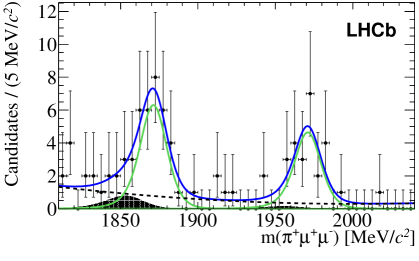
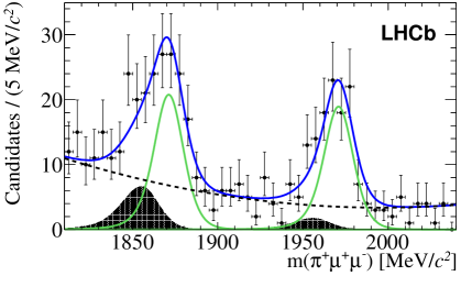
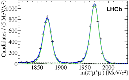
2pt (a) at 130 315
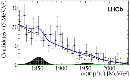
2pt (b) at 130 315 2pt (c) at 130 315 2pt (d) at 130 315 2pt (e) at 130 315

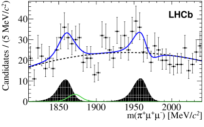
Figure 2: Invariant mass distributions for $D^{+}_{(s)}\!\rightarrow\mathup{{{\pi}}}^{+}\mathup{{{\mu}}}^{+}\mathup{{{\mu}}}^{-}$ candidates in the five $m(\mathup{{{\mu}}}^{+}\mathup{{{\mu}}}^{-})$ bins. Shown are the (a) low-$m(\mathup{{{\mu}}}^{+}\mathup{{{\mu}}}^{-})$, (b) $\mathup{{{\eta}}}$, (c) $\mathup{{{\rho}}}$/$\mathup{{{\omega}}}$, (d) $\mathup{{{\phi}}}$ (including trigger lines with $m(\mathup{{{\mu}}}^{+}\mathup{{{\mu}}}^{-})>1.0~{}{\mathrm{\,Ge\kern-0.90005ptV\!/}c^{2}}$), and (e) high-$m(\mathup{{{\mu}}}^{+}\mathup{{{\mu}}}^{-})$ regions. The data are shown as points (black) and the total PDF (dark blue line) is overlaid. The components of the fit are also shown: the signal (light green line), the peaking background (solid area) and the non-peaking background (dashed line).

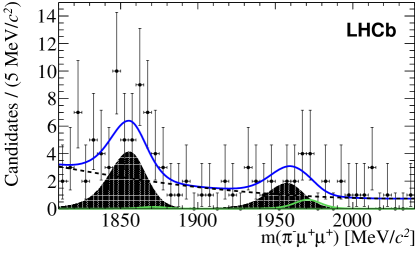
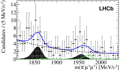
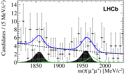
2pt (a) at 130 315 2pt (b) at 130 315 2pt (c) at 130 315 2pt (d) at 130 315

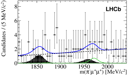
Figure 3: Invariant mass distributions for $D^{+}_{(s)}\!\rightarrow\mathup{{{\pi}}}^{-}\mathup{{{\mu}}}^{+}\mathup{{{\mu}}}^{+}$ in the four $m(\mathup{{{\pi}}}^{-}\mathup{{{\mu}}}^{+})$ regions. Shown are (a) bin 1, (b) bin 2, (c) bin 3, and (d) bin 4. The data are shown as black points and the total PDF (dark blue line) is overlaid. The components of the fit are also shown: the signal (light green line), the peaking background (solid area) and the non-peaking background (dashed line).

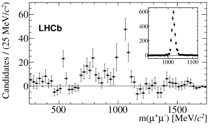
2pt (a) at 130 315 2pt (b) at 130 315

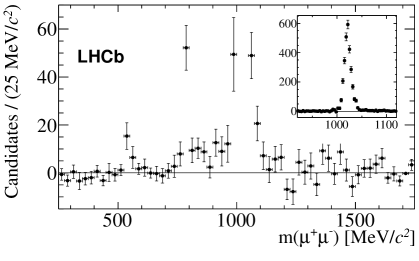
Figure 4: Background-subtracted m($\mathup{{{\mu}}}^{+}\mathup{{{\mu}}}^{-}$) spectrum of (a) $D^{+}\!\rightarrow\mathup{{{\pi}}}^{+}\mathup{{{\mu}}}^{+}\mathup{{{\mu}}}^{-}$ and (b) $D^{+}_{s}\!\rightarrow\mathup{{{\pi}}}^{+}\mathup{{{\mu}}}^{+}\mathup{{{\mu}}}^{-}$ candidates that pass the final selection. The inset shows the $\mathup{{{\phi}}}$ contribution, and the main figure shows the $\mathup{{{\eta}}}$ and the $\mathup{{{\rho}}}$/$\mathup{{{\omega}}}$ contributions. The non-peaking structure of the low and high-$m(\mathup{{{\mu}}}^{+}\mathup{{{\mu}}}^{-})$ regions is also visible.

5 Branching fraction determination

The $D^{+}_{(s)}\!\rightarrow\mathup{{{\pi}}}^{+}\mathup{{{\mu}}}^{+}\mathup{{{\mu}}}^{-}$ and $D^{+}_{(s)}\!\rightarrow\mathup{{{\pi}}}^{-}\mathup{{{\mu}}}^{+}\mathup{{{\mu}}}^{+}$ branching fractions are calculated using

$${{\cal B}(D^{+}_{(s)}\!\rightarrow\pi\mathup{{{\mu}}}\mathup{{{\mu}}})}=\frac{N_{D^{+}_{(s)}\!\rightarrow\pi\mathup{{{\mu}}}\mathup{{{\mu}}}}}{N_{D^{+}_{(s)}\!\rightarrow\mathup{{{\pi}}}^{+}(\mathup{{{\phi}}}\rightarrow\mathup{{{\mu}}}^{+}\mathup{{{\mu}}}^{-})}}\times\frac{\epsilon_{D^{+}_{(s)}\!\rightarrow\mathup{{{\pi}}}^{+}(\mathup{{{\phi}}}\rightarrow\mathup{{{\mu}}}^{+}\mathup{{{\mu}}}^{-})}}{\epsilon_{D^{+}_{(s)}\!\rightarrow\pi\mathup{{{\mu}}}\mathup{{{\mu}}}}}\times{{\cal B}(D^{+}_{(s)}\!\rightarrow\mathup{{{\pi}}}^{+}(\mathup{{{\phi}}}\rightarrow\mathup{{{\mu}}}^{+}\mathup{{{\mu}}}^{-}))},$$ (3)

where $D^{+}_{(s)}\!\rightarrow\pi\mathup{{{\mu}}}\mathup{{{\mu}}}$ represents either $D^{+}_{(s)}\!\rightarrow\mathup{{{\pi}}}^{+}\mathup{{{\mu}}}^{+}\mathup{{{\mu}}}^{-}$ or $D^{+}_{(s)}\!\rightarrow\mathup{{{\pi}}}^{-}\mathup{{{\mu}}}^{+}\mathup{{{\mu}}}^{+}$. The relevant signal yield and efficiency are given by $N_{D^{+}_{(s)}\!\rightarrow\pi\mathup{{{\mu}}}\mathup{{{\mu}}}}$ and $\epsilon_{D^{+}_{(s)}\!\rightarrow\pi\mathup{{{\mu}}}\mathup{{{\mu}}}}$, respectively, and the relevant control mode yield and efficiency are given by $N_{D^{+}_{(s)}\!\rightarrow\mathup{{{\pi}}}^{+}(\mathup{{{\phi}}}\rightarrow\mathup{{{\mu}}}^{+}\mathup{{{\mu}}}^{-})}$ and $\epsilon_{D^{+}_{(s)}\!\rightarrow\mathup{{{\pi}}}^{+}(\mathup{{{\phi}}}\rightarrow\mathup{{{\mu}}}^{+}\mathup{{{\mu}}}^{-})}$, respectively.

The efficiency of the signal decay mode and the control mode include the efficiencies of the geometrical acceptance of the detector, track reconstruction, muon identification, selection, and trigger. The accuracy with which the simulation reproduces the track reconstruction and identification is limited. For that reason, the corresponding efficiencies are also studied in real data. A tag and probe technique applied to $B\rightarrow J/\psi X$ decays provides a large sample of unambiguous muons to determine the tracking and muon identification efficiencies. The pion identification is studied using $D^{*+}\rightarrow\mathup{{{\pi}}}^{+}(D^{0}\rightarrow K^{-}\mathup{{{\pi}}}^{+})$ decays. The efficiencies observed as a function of the particle momentum and pseudorapidity and of the track multiplicity in the event are used to correct the efficiencies determined by the simulation. The correction to the efficiency ratio is typically of the order of 2% in each $m(\mathup{{{\mu}}}^{+}\mathup{{{\mu}}}^{-})$ or $m(\mathup{{{\pi}}}^{-}\mathup{{{\mu}}}^{+})$ region. Small relative corrections are expected since the signal and control modes share almost identical final states.

6 Systematic uncertainties

Systematic uncertainties in the calculation of the signal branching fractions arise due to imperfect knowledge of the control mode branching fraction, the efficiency ratio, and the yield ratio.

A systematic uncertainty of the order 10% accompanies the branching fraction of the control mode $D^{+}_{(s)}\!\rightarrow\mathup{{{\pi}}}^{+}(\mathup{{{\phi}}}\rightarrow\mathup{{{\mu}}}^{+}\mathup{{{\mu}}}^{-})$ and is the dominant source of the systematic uncertainty on the branching fraction measurement.

A systematic uncertainty affecting the efficiency ratio is due to the geometrical acceptance of the detector, which depends on the angular distributions of the final state particles, and thus on the decay model. By default, signal decays are simulated with a phase-space model. A conservative 1% uncertainty is determined by recalculating the acceptance assuming a flat $m(\mathup{{{\mu}}}^{+}\mathup{{{\mu}}}^{-})$ distribution.

The uncertainties on the tracking and particle identification corrections also affect the efficiency ratio and involve statistical components due to the size of the data samples and systematic uncertainties inherent in the techniques employed to determine the corrections. The corrections depend upon the choice of control sample, the selection and trigger requirements applied to this sample, and the precise definition of the probe tracks. The binning used to weight the efficiency as a function of the momentum, pseudorapity and multiplicity is varied to evaluate the uncertainty. The uncertainty in the choice of phase space model is accounted for by comparing the efficiency corrections in the extreme bins of the $m(\mathup{{{\mu}}}^{+}\mathup{{{\mu}}}^{-})$ or $m(\mathup{{{\pi}}}^{-}\mathup{{{\mu}}}^{+})$ distributions. In total, the uncertainty due to particle reconstruction and identification is found to be 4.2% across all bins.

Also affecting the efficiency ratio is the fact that the offline selection is not perfectly described by simulation. The systematic uncertainty is estimated by smearing track properties to reproduce the distributions observed in data, using $D^{+}_{(s)}\!\rightarrow\mathup{{{\pi}}}^{+}(\mathup{{{\phi}}}\rightarrow\mathup{{{\mu}}}^{+}\mathup{{{\mu}}}^{-})$ decays as a reference. The corresponding variation in the efficiency ratio indicates an uncertainty of 4%. Also, the trigger requirements imposed to select the signal are varied in order to test the imperfect simulation of the online reconstruction and $3\%$ uncertainty is deduced. The sources of uncertainty discussed so far are given in Table 3.

Final uncertainty on the efficiency ratio arises due to the finite size of the simulated samples. It is calculated separately in each $m(\mathup{{{\mu}}}^{+}\mathup{{{\mu}}}^{-})$ and $m(\mathup{{{\pi}}}^{-}\mathup{{{\mu}}}^{+})$ bin. These contributions are included in the systematic uncertainties shown in Table 4.

The systematic uncertainties affecting the yield ratio are taken into account when the branching fraction limits are calculated. The shapes of the signal peaks are assumed to be the same in all $m(\mathup{{{\mu}}}^{+}\mathup{{{\mu}}}^{-})$ and $m(\mathup{{{\pi}}}^{-}\mathup{{{\mu}}}^{+})$ bins. A 10% variation of the width of the Gaussian-like PDF, seen in simulation, is taken into account for variation across the bins. In each bin, the shape of the $D^{+}_{(s)}\!\rightarrow\mathup{{{\pi}}}^{+}\mathup{{{\pi}}}^{+}\mathup{{{\pi}}}^{-}$ peaking background is taken from a simultaneous fit to a larger sample to which looser $\mathrm{DLL}_{\mathup{{{\mu}}}\pi}$ criteria is applied. As simulation shows the shape of the PDF is altered by a $\mathrm{DLL}_{\mathup{{{\mu}}}\pi}$ requirement. A variation in the peaking background’s fitted width equal to 20% is applied as a systematic uncertainty. The pion-to-muon misidentification rate is assumed to be the same in all bins. Simulation suggests that a systematic variation of 20% in this quantity is conservative. Contributions to the yield ratio systematic uncertainty are found to increase the upper limit on the branching fraction by around 10%.

Table 3: Relative systematic uncertainties averaged over all bins and decay modes for the control mode branching fraction and efficiency ratio. The number in parentheses refers to the $D^{+}_{s}$ decay.

Source	Uncertainty (%)
Geometric acceptance	1.0
Track reconstruction and PID	4.2
Stripping and BDT efficiency	4.0
Trigger efficiency	3.0
$\cal B$($D^{+}_{(s)}$ $\rightarrow$ $\mathup{{{\pi}}}^{+}$ $\mathup{{{\phi}}}$ ($\mathup{{{\mu}}}^{+}\mathup{{{\mu}}}^{-}$)) uncertainty	8.1 (10.9)

Table 4: Total systematic uncertainty in each $m(\mathup{{{\mu}}}^{+}\mathup{{{\mu}}}^{-})$ and $m(\mathup{{{\pi}}}^{-}\mathup{{{\mu}}}^{+})$ bin with the uncertainty on the control mode branching fraction, the efficiency ratio and the statistical uncertainty stemming from the size of the simulated samples added in quadrature. The numbers in parentheses refer to the $D^{+}_{s}$ decay.

Bin description	$D^{+}_{(s)}\!\rightarrow\mathup{{{\pi}}}^{+}\mathup{{{\mu}}}^{+}\mathup{{{\mu}}}^{-}$ (%)	$D^{+}_{(s)}\!\rightarrow\mathup{{{\pi}}}^{-}\mathup{{{\mu}}}^{+}\mathup{{{\mu}}}^{+}$ (%)
low-$m(\mathup{{{\mu}}}^{+}\mathup{{{\mu}}}^{-})$	11.8 (16.9)
high-$m(\mathup{{{\mu}}}^{+}\mathup{{{\mu}}}^{-})$	11.2 (15.5)
bin 1		11.1 (17.0)
bin 2		10.9 (16.4)
bin 3		11.1 (16.0)
bin 4		11.3 (16.0)

7 Results

The compatibility of the observed distribution of candidates with a signal plus background or background-only hypothesis is evaluated using the $\mathrm{CL}_{s}$ method [27, 28]. The method provides two estimators: $\mathrm{CL}_{s}$, a measure of the compatibility of the observed distribution with the signal hypothesis, and $\mathrm{CL}_{b}$, a measure of the compatibility with the background-only hypothesis. The systematic uncertainties are included in the $\mathrm{CL}_{s}$ method using the techniques described in Ref. [27, 28].

Upper limits on the $D^{+}\!\rightarrow\mathup{{{\pi}}}^{+}\mathup{{{\mu}}}^{+}\mathup{{{\mu}}}^{-}$ and $D^{+}\!\rightarrow\mathup{{{\pi}}}^{-}\mathup{{{\mu}}}^{+}\mathup{{{\mu}}}^{+}$ branching fractions are determined using the observed distribution of $\mathrm{CL}_{s}$ as a function of the branching fraction in each $m(\mathup{{{\mu}}}^{+}\mathup{{{\mu}}}^{-})$ or $m(\mathup{{{\pi}}}^{-}\mathup{{{\mu}}}^{+})$ bin. Total branching fractions are found using the same method and by considering the fraction of simulated signal candidates in each $m(\mathup{{{\mu}}}^{+}\mathup{{{\mu}}}^{-})$ or $m(\mathup{{{\pi}}}^{-}\mathup{{{\mu}}}^{+})$ bin. The simulated signal assumes a phase-space model for the non-resonant decays. The observed distribution of $\mathrm{CL}_{s}$ as a function of the total branching fraction for $D^{+}\!\rightarrow\mathup{{{\pi}}}^{+}\mathup{{{\mu}}}^{+}\mathup{{{\mu}}}^{-}$ is shown in Fig. 5. The upper limits at 90% and 95% $\mathrm{CL}$ and the p-values $(1-\mathrm{CL}_{b})$ for the the background-only hypothesis are shown in Table 5 .

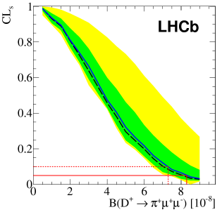
Figure 5: Observed (solid curve) and expected (dashed curve) $\mathrm{CL}_{s}$ values as a function of $\cal B$($D^{+}\!\rightarrow\mathup{{{\pi}}}^{+}\mathup{{{\mu}}}^{+}\mathup{{{\mu}}}^{-}$). The green (yellow) shaded area contains the $\pm 1\sigma$ ($\pm 2\sigma$) interval of possible results compatible with the expected value if only background is observed. The upper limits at the 90% (95%) $\mathrm{CL}$ are indicated by the dashed (solid) line.

Table 5: Upper limits in each $m(\mathup{{{\mu}}}^{+}\mathup{{{\mu}}}^{-})$ and $m(\mathup{{{\pi}}}^{-}\mathup{{{\mu}}}^{+})$ bin and total branching fractions at the 90% and 95% $\mathrm{CL}$ and p-values for the background-only hypothesis.

Decay	Bin	$90\%\,[\times 10^{-8}]$	$95\%\,[\times 10^{-8}]$	p-value
$D^{+}\!\rightarrow\mathup{{{\pi}}}^{+}\mathup{{{\mu}}}^{+}\mathup{{{\mu}}}^{-}$	low-$m(\mathup{{{\mu}}}^{+}\mathup{{{\mu}}}^{-})$	2.0	2.5	0.74
	high-$m(\mathup{{{\mu}}}^{+}\mathup{{{\mu}}}^{-})$	2.6	2.9	0.42
	Total	7.3	8.3	0.42
$D^{+}_{s}\!\rightarrow\mathup{{{\pi}}}^{+}\mathup{{{\mu}}}^{+}\mathup{{{\mu}}}^{-}$	low-$m(\mathup{{{\mu}}}^{+}\mathup{{{\mu}}}^{-})$	6.9	7.7	0.78
	high-$m(\mathup{{{\mu}}}^{+}\mathup{{{\mu}}}^{-})$	16.0	18.6	0.41
	Total	41.0	47.7	0.42
$D^{+}\!\rightarrow\mathup{{{\pi}}}^{-}\mathup{{{\mu}}}^{+}\mathup{{{\mu}}}^{+}$	bin 1	1.4	1.7	0.32
	bin 2	1.1	1.3	0.61
	bin 3	1.3	1.5	0.94
	bin 4	1.3	1.5	0.97
	Total	2.2	2.5	0.86
$D^{+}_{s}\!\rightarrow\mathup{{{\pi}}}^{-}\mathup{{{\mu}}}^{+}\mathup{{{\mu}}}^{+}$	bin 1	6.2	7.6	0.34
	bin 2	4.4	5.3	0.51
	bin 3	6.0	7.3	0.32
	bin 4	7.5	8.7	0.41
	Total	12.0	14.1	0.12

8 Conclusions

A search for the $D^{+}_{(s)}\!\rightarrow\mathup{{{\pi}}}^{+}\mathup{{{\mu}}}^{+}\mathup{{{\mu}}}^{-}$ and $D^{+}_{(s)}\!\rightarrow\mathup{{{\pi}}}^{-}\mathup{{{\mu}}}^{+}\mathup{{{\mu}}}^{+}$ decays has been conducted using proton-proton collision data, corresponding to an integrated luminosity of 1.0 $\mbox{\,fb}^{-1}$, at $\sqrt{s}=7$ $\mathrm{\,Te\kern-1.00006ptV}$ recorded by the LHCb experiment. Limits are set on branching fractions in several $m(\mathup{{{\mu}}}^{+}\mathup{{{\mu}}}^{-})$ and $m(\mathup{{{\pi}}}^{-}\mathup{{{\mu}}}^{+})$ bins and on the total branching fraction excluding the resonant contributions assuming a phase-space model. These results are the most stringent to date and represent an improvement by a factor of fifty compared to previous results. The observed data, away from resonant structures, is compatible with the background-only hypothesis, and no enhancement is observed. The $90\%\,(95)\%$ $\mathrm{CL}$ limits on the branching fractions are

$$\mathcal{{\cal B}}(D^{+}\!\rightarrow\mathup{{{\pi}}}^{+}\mathup{{{\mu}}}^{+}\mathup{{{\mu}}}^{-})<7.3\,(8.3)\times 10^{-8},$$

$$\mathcal{{\cal B}}(D^{+}_{s}\!\rightarrow\mathup{{{\pi}}}^{+}\mathup{{{\mu}}}^{+}\mathup{{{\mu}}}^{-})<4.1\,(4.8)\times 10^{-7},$$

$$\mathcal{{\cal B}}(D^{+}\!\rightarrow\mathup{{{\pi}}}^{-}\mathup{{{\mu}}}^{+}\mathup{{{\mu}}}^{+})<2.2\,(2.5)\times 10^{-8},$$

$$\mathcal{{\cal B}}(D^{+}_{s}\!\rightarrow\mathup{{{\pi}}}^{-}\mathup{{{\mu}}}^{+}\mathup{{{\mu}}}^{+})<1.2\,(1.4)\times 10^{-7}.$$

References

- [1] S. Fajfer and S. Prelovsek, Search for new physics in rare D decays, Conf. Proc. C060726 (2006) 811, arXiv:hep-ph/0610032
- [2] Belle collaboration, K. Abe et al., Observation of the decay , Phys. Rev. Lett. 88 (2002) 021801, arXiv:hep-ex/0109026
- [3] HyperCP collaboration, H. Park et al., Observation of the decay and measurements of the branching ratios for , Phys. Rev. Lett. 88 (2002) 111801, arXiv:hep-ex/0110033
- [4] S. Fajfer, S. Prelovsek, and P. Singer, Rare charm meson decays and in SM and MSSM, Phys. Rev. D64 (2001) 114009, arXiv:hep-ph/0106333
- [5] S. Fajfer, N. Kosnik, and S. Prelovsek, Updated constraints on new physics in rare charm decays, Phys. Rev. D76 (2007) 074010, arXiv:0706.1133
- [6] A. Paul, I. I. Bigi, and S. Recksiegel, On within the Standard Model and frameworks like the littlest Higgs model with T parity, Phys. Rev. D83 (2011) 114006, arXiv:1101.6053
- [7] M. Artuso et al., , and decays, Eur. Phys. J. C57 (2008) 309, arXiv:0801.1833
- [8] D0 collaboration, V. Abazov et al., Search for flavor-changing-neutral-current meson decays, Phys. Rev. Lett. 100 (2008) 101801, arXiv:0708.2094
- [9] FOCUS Collaboration, J. Link et al., Search for rare and forbidden three body dimuon decays of the charmed mesons and , Phys. Lett. B572 (2003) 21, arXiv:hep-ex/0306049
- [10] E. Majorana, Teoria simmetrica dell’elettrone e del positrone, Nuovo Cim. 14 (1937) 171
- [11] BaBar collaboration, J. Lees et al., Searches for rare or forbidden semileptonic charm decays, Phys. Rev. D84 (2011) 072006, arXiv:1107.4465
- [12] LHCb collaboration, R. Aaij et al., Searches for Majorana neutrinos in decays, arXiv:1201.5600
- [13] Particle Data Group, J. Beringer et al., Review of particle physics, Phys. Rev. D86 (2012) 010001
- [14] LHCb collaboration, A. A. Alves Jr. et al., The LHCb detector at the LHC, JINST 3 (2008) S08005
- [15] M. Adinolfi et al., Performance of the LHCb RICH detector at the LHC, arXiv:1211.6759
- [16] R. Aaij et al., The LHCb trigger and its performance, arXiv:1211.3055, to appear in JINST
- [17] T. Sjöstrand, S. Mrenna, and P. Skands, PYTHIA 6.4 physics and manual, JHEP 05 (2006) 026, arXiv:hep-ph/0603175
- [18] I. Belyaev et al., Handling of the generation of primary events in Gauss, the LHCb simulation framework, Nuclear Science Symposium Conference Record (NSS/MIC) IEEE (2010) 1155
- [19] D. J. Lange, The EvtGen particle decay simulation package, Nucl. Instrum. Meth. A462 (2001) 152
- [20] GEANT4 collaboration, J. Allison et al., Geant4 developments and applications, IEEE Trans. Nucl. Sci. 53 (2006) 270
- [21] GEANT4 collaboration, S. Agostinelli et al., GEANT4: A simulation toolkit, Nucl. Instrum. Meth. A506 (2003) 250
- [22] M. Clemencic et al., The LHCb simulation application, Gauss: design, evolution and experience, J. of Phys. Conf. Ser. 331 (2011) 032023
- [23] L. Breiman, J. H. Friedman, R. A. Olshen, and C. J. Stone, Classification and regression trees, Wadsworth international group, Belmont, California, USA, 1984
- [24] B. P. Roe et al., Boosted decision trees as an alternative to artificial neural networks for particle identification, Nucl. Instrum. Meth. A543 (2005) 577, arXiv:physics/0408124
- [25] A. Hoecker et al., TMVA: Toolkit for Multivariate Data Analysis, PoS ACAT (2007) 040, arXiv:physics/0703039
- [26] M. Pivk and F. R. Le Diberder, sPlot: a statistical tool to unfold data distributions, Nucl. Instrum. Meth. A555 (2005) 356, arXiv:physics/0402083
- [27] A. Read, Presentation of search results: the CLs technique, J. Phys. G28 (2002) 2693
- [28] T. Junk, Confidence level computation for combining searches with small statistics, Nucl. Instrum. Meth. A434 (1999) 435, arXiv:hep-ex/9902006