Soft singularity crossing and transformation of matter properties

Abstract

We investigate particular cosmological models, based either on tachyon fields or on perfect fluids, for which soft future singularities arise in a natural way. Our main result is the description of a smooth crossing of the soft singularity in models with an anti-Chaplygin gas or with a particular tachyon field in the presence of dust. Such a crossing is made possible by certain transformations of matter properties. Some of these cosmological evolutions involving tachyons are compatible with SNIa data. We compute numerically their dynamics involving a first soft singularity crossing, a turning point and a second soft singulatity crossing during recollapse, ending in a Big Crunch singularity.

I Introduction

In a recent paper Paradox we have investigated the possibility of soft singularity crossing in a model where a flat Friedmann universe was filled with dust and anti-Chaplygin gas. A soft singularity appears in an expanding universe when the pressure of the anti-Chaplygin gas diverges, causing $\ddot{a}\rightarrow-\infty$ ($a$ is the scale factor and the dot denotes the derivative with respect to cosmic time), while $a$ and $\dot{a}$ remain finite. The energy density of the anti-Chaplygin gas vanishes at the singularity while the energy density of dust remains finite there, thus implying $\dot{a}>0$. The geodesic equations remain regular at the singularity and, therefore, they can be continued through. This allows the universe to cross the soft singularity. Then, a smooth evolution of the universe would require further expansion. However, in this case the energy density of the anti-Chaplygin gas would become imaginary and hence ill defined. This contradiction and the fact that the geodesics can be continued through leads to a paradox. In Paradox we have solved this paradox by relaxing the smoothness condition, leading to the redefinition of cosmological quantities as distributions. With this redefinition, it turns out that the universe can revert abruptly from expansion to contraction.

In the present work we study an alternative possibility for the continuation of geodesics across the singularity, requiring the continuity of the spacetime evolution at the expense of certain transformations of matter properties.

The paper is organized as follows. In Sec. II we discuss the sudden singularities that arise in a class of flat Friedmann models such as those describing universes filled with the anti-Chaplygin gas without or with dust, or driven by a specific tachyon field tach0 , again without and with dust. In Sec. III we describe the crossing of a soft singularity with accompanying transformations of matter in the above-mentioned models. Section IV presents numerical results of the evolution of universes filled with a tachyon field and dust, compatible with SNIa data. Concluding remarks are presented in Sec. V. We choose units $c=1$ and $8\pi G/3=1$.

II Sudden singularities in flat Friedmann universes

The line element squared of a flat Friedmann universe can be written as

$$ds^{2}=dt^{2}-a^{2}\left(t\right)\sum_{\alpha}\left(dx^{\alpha}\right)^{2},$$ (1)

where $x^{\alpha}$ ($\alpha=1,2,3$) are spatial Cartesian coordinates. The evolution of the universe is governed by the Raychaudhuri (second Friedmann) equation

$$\dot{H}=-\frac{3}{2}\left(\rho+p\right),$$ (2)

and by the continuity equation for the fluid,

$$\dot{\rho}+3H\left(\rho+p\right)=0,$$ (3)

where, as usual, $\rho$ is the energy density, $p$ is the pressure of matter and $H\equiv\dot{a}/a$ is the Hubble parameter. The first Friedmann equation is

$$H^{2}=\rho.$$ (4)

Sudden singularities are characterized by finite $H_{S}$ and $\dot{H}_{S}=-\infty$ (finite $\dot{a}_{S}$ and $\ddot{a}_{S}=-\infty$) at some finite scale factor $a_{S}$. Here, the subscript $S$ denotes the respective quantities evaluated at the singularity. These conditions can be formulated in terms of energy density and pressure of the fluid. The Friedmann (4) and Raychaudhuri (2) equations show that the total energy density $\rho_{S}$ is nonnegative and finite while the pressure diverges $p_{S}=\infty$.

It was shown in Lazkoz , tach2 and Paradox that the geodesics can be continued across such sudden singularities as the geodesic equations are regular there. The singularity is weak (soft) according to the definitions of both Tipler Tipler and Królak Krolak . Although the tidal forces become infinite, the extended objects are not necessarily crushed when reaching the singularity.

II.1 Big brake

A special case of sudden singularity is the Big Brake singularity, occurring when the energy density vanishes at the singularity, $\rho_{S}=0$ tach0 .

II.1.1 Anti-Chaplygin gas

One of the simplest models where the Big Brake singularity arises is the anti-Chaplygin gas tach0 . This is a perfect fluid with the equation of state

$$p=\frac{A}{\rho}~{},$$ (5)

where $A>0$, as opposed to the Chaplygin gas we-Chap ; we-Chap1 which has the equation of state $p=-A/\rho$. The equation of state (5) arises, for example, in the theory of wiggly strings wiggly .

Applied to the anti-Chaplygin gas, the continuity equation (3) gives the following dependence of the energy density on the scale factor:

$$\rho_{ACh}=\sqrt{\frac{B}{a^{6}}-A}~{},$$ (6)

where $B$ is a positive constant, which determines the initial condition. When the scale factor approaches the value

$$a_{S}=\left(\frac{B}{A}\right)^{\frac{1}{6}},$$ (7)

during the expansion of the universe, the energy density of the anti-Chaplygin gas vanishes, and its pressure grows to infinity. Accordingly, the deceleration also becomes infinite.

As it was shown in Paradox , after crossing of this singularity the universe starts contracting towards a Big Crunch.

II.1.2 The tachyon field with trigonometric potential and transition to a Born-Infeld type pseudotachyon field

A Big Brake singularity was first found in a specific tachyon model introduced in tach0 . The Lagrangian density of a tachyon field is Sen

$$L=-V(T)\sqrt{1-g^{ij}\left(\partial_{i}T\right)\left(\partial_{j}T\right)},$$ (8)

where $V(T)$ is a potential. For a spatially homogeneous field $T(t)$, the expression (8) becomes

$$L=-V(T)\sqrt{1-g^{tt}\dot{T}^{2}}.$$ (9)

This field corresponds to an ideal fluid with energy density

$$\rho_{T}=\frac{V(T)}{\sqrt{1-\dot{T}^{2}}},$$ (10)

and pressure

$$p_{T}=-V(T)\sqrt{1-\dot{T}^{2}}.$$ (11)

The Lagrangian density as well as $\rho_{T}$ and $p_{T}$ are well defined for $\dot{T}^{2}\leq 1$. The field equation is

$$\frac{\ddot{T}}{1-\dot{T}^{2}}+3H\dot{T}+\frac{V_{,T}}{V}=0.$$ (12)

The following potential was studied in tach0 :

$$V(T)=\frac{\Lambda\sqrt{1-(1+k)y^{2}}}{1-y^{2}},$$ (13)

with

$$y=\cos\left[\frac{3}{2}{\sqrt{\Lambda\,(1+k)}\,T}\right],$$ (14)

where $\Lambda>0$ and $-1<k<1$ are model parameters. The case $k>0$ is of particular interest, because it reveals two unusual features: a self-transformation of the tachyon into a pseudotachyon field and the appearance of a Big Brake cosmological singularity. For $k>0$, the potential (13)–(14), is well defined in the range

$$-y_{\ast}<y<y_{\ast},\ \text{or}\ T_{4}>{T}>T_{3},$$ (15)

where

$$y_{\ast}=(1+k)^{-1/2},$$ (16)

$$T_{3}=\frac{2}{3\sqrt{\Lambda(1+k)}}\arccos(1+k)^{-1/2},$$ (17)

$$T_{4}=\frac{2}{3\sqrt{\Lambda(1+k)}}\arccos\left[\pi-(1+k)^{-1/2}\right].$$ (18)

Note that the dynamical system is invariant under the simultaneous change

$$y\rightarrow-y\ ,\ \ \dot{T}\rightarrow-\dot{T}\ .$$ (19)

Since $V\geq 0$ the pressure is negative allowing for an accelerated expansion of the universe. When they reach the attractive critical point $(y=0,\dot{T}=0)$, the trajectories correspond to an exact de Sitter expansion of the universe. The lines $\dot{T}=\pm 1$ (with the exception of the corner points ($\pm y_{\ast}$, $\dot{T}=\pm 1$)) in the ($T$,$\dot{T}$) space correspond to a standard Big Bang singularity (see Fig. 5 of tach2 , which reproduces Fig. 4 in tach0 ).

However, some trajectories can reach the corner points where the geometry is not singular. Hence, the trajectories can be continued across these corner points, beyond which $|\dot{T}|^{2}$ becomes larger than $1$. The potential $V$ and the kinetic term in the Lagrangian density (8) become imaginary across the corner points; however their product remains real. Thus for $\dot{T}^{2}>1$ the correct Lagrangian density (describing a Born-Infeld type pseudotachyon field) is

$$L=W(T)\sqrt{g^{tt}\dot{T}^{2}-1},$$ (20)

where

$$W(T)=\frac{\Lambda\sqrt{(1+k)y^{2}-1}}{1-y^{2}}.$$ (21)

This Lagrangian is well defined in the ranges

$$-1<y<-y_{\ast},\ \text{or }T_{\max}>{T}>T_{4}$$ (22)

and

$$y_{\ast}<y<1,\ \text{ or }T_{3}>{T}>0,$$

with

$$T_{\max}=\pi/3\sqrt{\Lambda(1+k)}.$$ (23)

The energy density and pressure are now

$$\rho_{T}=\frac{W\left(T\right)}{\sqrt{\dot{T}^{2}-1}},$$ (24)

$$p_{T}=W\left(T\right)\sqrt{\dot{T}^{2}-1}.$$ (25)

Since the pressure is positive, the expansion of the universe is slowing down. The field equation is

$$\frac{\ddot{T}}{1-\dot{T}^{2}}+3H\dot{T}+\frac{W_{,T}}{W}=0.$$ (26)

The universe runs into a soft singularity somewhere in the ranges $y_{\ast}<y<1$ as ${\dot{T}\rightarrow-\infty}$ or $-1<y<-y_{\ast}$ as ${\dot{T}\rightarrow\infty}$ tach0 . From Eqs. (21)-(25), the potential $W$ is finite and $\rho_{T}\rightarrow 0$, $p_{T}\rightarrow\infty$ at the soft singularity. Equivalently, this means that $H_{S}=0$, while $\dot{H}_{S}=-\infty$. It was shown in tach2 that the evolution of the universe can be continued across the singularity, where the universe starts recollapsing and eventually ends in a Big Crunch singularity.

II.2 Introducing a dust component

The dust is a perfect fluid with vanishing pressure, whose energy density is

$$\rho_{m}=\frac{\rho_{m,0}}{a^{3}},~{}$$ (27)

where $\rho_{m,0}$ is a positive constant, characterizing the quantity of matter in the universe today ($a_{0}=1$). Therefore, if a cosmological model with dust evolves into a sudden singularity the energy density of dustlike matter remains finite $\left(\rho_{m}\right)_{S}>0$. Then, the Hubble parameter does not vanish at the singularity as in the case of the Big Brake. This makes it more difficult and delicate to describe what happens after reaching a soft singularity.

II.2.1 Anti-Chaplygin gas

A soft singularity arising in a two-fluid model containing dust and anti-Chaplygin gas was investigated in Paradox . The Hubble parameter is positive at the singularity, requiring a further expansion of the universe. Then a paradox arises: if the universe continues to expand, beyond the singularity the expression under the sign of the square root in Eq. (6) becomes negative and the energy density of the anti-Chaplygin gas becomes ill defined.

A mathematically consistent way out of this situation is an abrupt replacement of the cosmological expansion by a contraction at the price of introducing distributional cosmological quantities Paradox .

In the next section, we investigate an alternative possibility requiring the smoothness in the evolution of the Hubble parameter but allowing for a change in the equation of state (5).

II.2.2 Born-Infeld type pseudotachyon field with trigonometric potential

In the model suggested in tach0 the Born-Infeld type pseudotachyon field runs into a soft Big Brake singularity at some point during the expansion of the universe. What happens however in the presence of a dust component? Does the universe still run into a soft singularity?

In order to answer this question, we rewrite Eq. (26) as

$$\ddot{T}=(\dot{T}^{2}-1)\left(3H\dot{T}+\frac{W_{,T}}{W}\right).$$ (28)

In the left lower and in the right upper stripes (see Fig. 4 of tach0 ), where the trajectories describe the expansion of the universe after the transformation of the tachyon into the pseudotachyon field, the signs of $\ddot{T}$, of $\dot{T}$ and of the term $W_{,T}/W$ coincide. A detailed analysis based on this fact was carried out in tach0 and led to the conclusion that the universe encounters the singularity as $T\rightarrow T_{S}$ ($T_{S}>0$ or $T_{S}>T_{max}$) , $|\dot{T}|\rightarrow\infty$. The presence of dust cannot alter this because it increases the influence of the term $3H\dot{T}$, and hence, accelerates the encounter with the singularity. Indeed, consider two trajectories, crossing one of the corners (i.e., undergoing the tachyon-pseudotachyon transition) under the same angle in phase space (cf. Fig. 4 in tach0 ), one in the absence of dust, the other in the presence of dust. For both trajectories the signs of $\ddot{T}$ and of $\dot{T}$ in (28) coincide and the increase that the value of $H$ undergoes when dust is present makes the growing of $|\dot{T}|$ more abrupt. On the other hand, the evolution of the tachyon field, approaching the corner point is slowed down by the presence of dust, because, in this case (inside the rectangle of the phase space) $(\dot{T}^{2}-1)$ is negative and therefore $\ddot{T}$ and $\dot{T}$ have opposite signs. Summing up, we may say that the presence of dust accelerates the evolution of the pseudotachyon whereas it slows down the evolution of tachyon.

What is important is that the presence of dust changes in an essential way the time dependence of the pseudotachyon field close to the singularity. Indeed, as it was shown in tach2 , in the absence of dust one has

$$T=T_{BB}\pm\left(\frac{4}{3W(T_{BB})}\right)^{1/3}(t_{BB}-t)^{1/3},$$ (29)

(see Eq. (29) in tach2 ). The upper (lower) sign corresponds to the left lower (right upper) strip in Fig. 4 of tach0 , where $\lim_{t\rightarrow t_{BB}}\dot{T}=-\infty$ ( $\lim_{t\rightarrow t_{BB}}\dot{T}=\infty$). In the presence of dust one has, instead,

$$T=T_{S}\pm\sqrt{\frac{2}{3H_{S}}}\sqrt{t_{S}-t},$$ (30)

where $H_{S}$ is the nonvanishing value of the Hubble parameter given by

$$H_{S}=\sqrt{\frac{\rho_{m,0}}{a_{S}^{3}}}.$$ (31)

Here we have taken advantage of the fact that in Eq. (28) the terms $1$ and $W_{,T}/W$ can be neglected with respect to $\dot{T}^{2}$ and $3H\dot{T}$, respectively. It is easy to see that a smooth continuation of expression (30) is impossible in contrast to the situation without dust (29).

Thus, the presence of dust is responsible for the appearance of similar paradoxes in both the anti-Chaplygin gas and tachyon models.

III Crossing the soft singularity and transformations of matter

As mentioned earlier (see Introduction of the present paper and the concluding remarks in Paradox ) the mathematically self-consistent scenario, based on the treatment of physical quantities as generalized functions and on the abrupt change of the expansion into a contraction, may look counterintuitive from the physical point of view. Indeed, such a behavior displays features which are analogous to the phenomenon of the absolutely elastic bounce of a hard ball from a rigid wall, as studied in classical mechanics. In the latter case, it is the velocity and the momentum of the ball which change their direction abruptly. Hence, an infinite force acts from the wall onto the ball during an infinitely small interval of time.

In reality, the absolutely elastic bounce is an idealization of a process taking place in a finite, though small, time-span, during which inelastic deformations of the ball and of the wall occur. This implies a more complex and realistic description of the dynamical process of interaction between the ball and the wall. Hence, we are naturally led to assume that something similar should occur also in the models of an anti-Chaplygin gas or a tachyon whenever dust is present. We expect that the smoothing of the process of the transition from an expanding to a contracting phase should include some (temporary) geometrically implied change of the equation of state of matter or of the form of the Lagrangian. We know that such changes have been considered in cosmology. For example, a tachyon–pseudo-tachhyon transformation, driven by the continuity of the cosmological evolution, took place in the tachyon model tach0 (see also subsection II.B.2 of the present paper). In a cosmological model with the phantom field with a cusped potential cusped , transformations between phantom and standard scalar field were considered. Thus, it is quite natural to assume that the process of crossing of the soft singularity should imply similar transformations.

However, the situation is now more complicated. It is not enough to require the continuity of the evolution of the cosmological radius and of the Hubble parameter. It is also necessary to make some hypotheses about changing the equation of state of matter or the form of the Lagrangian.

We solve the problem as follows. Considering first the anti-Chaplygin gas with dust, we require a minimal change in the form of the dependence of the energy density and of the pressure on the cosmological radius, upon crossing the soft singularity. This will require replacement of the anti-Chaplygin gas with a Chaplygin gas with negative energy density. Next, we consider the cosmological model based on a pseudotachyon field with constant potential and in the presence of dust. It is known that the energy-momentum tensor for such a pseudotachyon field coincides with that of the anti-Chaplygin gas (relating the Chaplygin gas to the tachyon field with constant potential was considered in FKS ). We derive how the pseudotachyon Lagrangian transforms using its kinship with the anti-Chaplygin gas. In this way, we arrive at a new type of Lagrangian, belonging to the “Born-Infeld family”. Finally, we extend this transformation to the case of the trigonometric potential.

III.1 Anti-Chaplygin gas

It follows from Eqs. (5) and (6) that the pressure of the anti-Chaplygin gas

$$p=\frac{A}{\sqrt{\frac{B}{a^{6}}-A}}$$ (32)

tends to $+\infty$ when the universe approaches the soft singularity, e.g. when the cosmological radius $a\rightarrow a_{S}$ (see Eq. (7)). Requiring the expansion to continue into the region $a>a_{S}$, while changing minimally the equation of state, we assume

$$p=\frac{A}{\sqrt{|\frac{B}{a^{6}}-A|}},$$ (33)

or, in other words,

$$p=\frac{A}{\sqrt{A-\frac{B}{a^{6}}}},\ \mathrm{for}\ a>a_{S}.$$ (34)

Thus, the pressure passes through $+\infty$ conserving its sign, thus providing in such a way the continuity of the cosmological evolution. It is crucial that $p$ does not change sign in order to keep a decelerated expansion. The energy density $\rho$ evolves continuously, and so does its derivative with respect to volume. Combining (34) with the energy conservation law (3) we obtain

$$\rho=-\sqrt{A-\frac{B}{a^{6}}},\ \mathrm{for}\ a>a_{S},$$ (35)

so that for $a>a_{S}$ the energy density and the pressure satisfy the Chaplygin gas equation of state

$$p=-\frac{A}{\rho}.$$ (36)

Therefore, at the singularity crossing, the anti-Chaplygin gas transforms into a Chaplygin gas with negative energy density. After crossing of the singularity the Friedmann equation is

$$H^{2}=\frac{\rho_{m,0}}{a^{3}}-\sqrt{A}\sqrt{1-\left(\frac{a_{S}}{a}\right)^{6}},$$ (37)

and it follows from Eq. (37) that, after achieving the point of maximal expansion $a=a_{\mathrm{max}}$, where

$$a_{\mathrm{max}}=\left(\frac{\rho_{m,0}^{2}}{A}+a_{S}^{6}\right)^{1/6},$$ (38)

the universe begins contracting. During this phase, as it achieves again $a=a_{S}$, it stumbles once more upon a soft singularity, whereupon the Chaplygin gas transforms itself back into anti-Chaplygin with positive energy density and the contraction continues until hitting the Big Crunch singularity.

Whereas in Paradox we envisaged an abrupt change from expansion to contraction through the singularity, with a jump in the Hubble parameter, we show here that a continuous transition to the collapsing phase is possible if the equation of state of the anti-Chaplygin gas has some kind of “phase transition” at the singularity.

III.2 Pseudotachyon field with a constant potential

For a pseudotachyon field with constant potential $W(T)=W_{0}$, the energy density (24) and the pressure (25) satisfy the anti-Chaplygin gas equation of state (5) with

$$A=W_{0}^{2}.$$ (39)

Solving the equation of motion for the pseudotachyon field (26) with $W(T)=W_{0}$, one finds

$$\dot{T}^{2}=\frac{1}{1-\left(\frac{a}{a_{S}}\right)^{6}}$$ (40)

and we see that a soft singularity arises at $a=a_{S}$ with $\dot{T}^{2}\rightarrow+\infty$.

The new Lagrangian, which gives the correct energy density and pressure satisfying a Chaplygin gas equation with negative energy density is

$$L=W_{0}\sqrt{g^{tt}\dot{T}^{2}+1},~{}~{}~{}~{}~{}~{}~{}~{}~{}~{}~{}~{}~{}~{}~{}~{}~{}a>a_{S}$$ (41)

giving

$$p=W_{0}\sqrt{\dot{T}^{2}+1}$$ (42)

and

$$\rho=-\frac{W_{0}}{\sqrt{\dot{T}^{2}+1}}.$$ (43)

Lagrangian (41) characterizes a new type of Born-Infeld field, which we may call “quasitachyon”.

For an arbitrary potential the Lagrangian reads

$$L=W(T)\sqrt{g^{tt}\dot{T}^{2}+1}~{}~{}~{}~{}~{}~{}~{}~{}~{}~{}~{}~{}~{}~{}~{}~{}~{}a>a_{S}$$ (44)

with equation of motion

$$\frac{\ddot{T}}{\dot{T}^{2}+1}+3H\dot{T}-\frac{W_{,T}}{W}=0$$ (45)

and energy density and pressure are, respectively,

$$\rho=-\frac{W(T)}{\sqrt{\dot{T}^{2}+1}}~{}$$ (46)

and

$$p=W(T)\sqrt{\dot{T}^{2}+1}.$$ (47)

If $W(T)=W_{0}$, the solution of equation (45) is

$$\dot{T}^{2}=\frac{1}{\left(\frac{a}{a_{S}}\right)^{6}-1},$$ (48)

and the energy density evolves as

$$\rho_{T}=-W_{0}\sqrt{1-\left(\frac{a_{S}}{a}\right)^{6}}.$$ (49)

The evolution of the universe coincides with that of a universe with anti-Chaplygin gas and dust.

Thus, the transformation from anti-Chaplygin to Chaplygin gas with negative energy density corresponds to a transition from a pseudotachyon field with Lagrangian (20) with constant potential $W(T)=W_{0}$ to a new Born-Infeld type quasitachyon field, with Lagrangian (41).

III.3 The tachyon model with trigonometric potential and dust

In the vicinity of the soft singularity, it is the “friction” term $3H\dot{T}$ in the equation of motion (26), which dominates over the potential term $W_{,T}/W$. Hence, the dependence of $W(T)$ on its argument is not essential and a pseudotachyon field approaching this singularity behaves like one with a constant potential. Thus, it is reasonable to assume that upon crossing the soft singularity the pseudotachyon transforms itself into a quasitachyon with Lagrangian (44) for any potential $W(T)$.

We now study the dynamics of the model with trigonometric potential (13)-(14) in the presence of dust.

The behavior of the quasitachyon field close to the soft singularity can be derived from Eq. (45) in the same way as the corresponding behavior of the pseudotachyon field derives from Eq. (28). In analogy with Eq. (30), we obtain the quasitachyon behavior

$$T=T_{S}\mp\sqrt{\frac{2}{3H_{S}}}\sqrt{t-t_{S}}$$ (50)

and the two formulas match with each other through the singularity.

In order to analyze the dynamics of the field in the presence of dust, it is convenient to concentrate ourselves on the processes as they occur, say, in the left lower strip of the phase diagram of the model, to facilitate comparison with earlier studies of the tachyon model dynamics without dust in tach0 ; tach2 . The relative signs in the equations of motion of the term with the second derivative $\ddot{T}$ and of the friction term $3H\dot{T}$ are opposite for pseudotachyons and quasitachyons. This means that after crossing the soft singularity the time derivative $\dot{T}$ grows while its absolute value decreases. At the same time the value of $T$ is decreasing while the potential $W(T)$, given by (21) is growing.

Hence the absolute value of the negative contribution to the energy density of the universe induced by the quasitachyon grows while the energy density of the dust decreases due to the expansion of the universe. Thus, at some moment the total energy density vanishes and the universe reaches the point of maximal expansion, after which the expansion is replaced by a contraction and the Hubble variable changes sign. The change of sign of the friction term $3H\dot{T}$ implies the value of $\dot{T}$ to decrease and at some finite moment of time the universe hits again the soft singularity when $\dot{T}\rightarrow-\infty$. Upon crossing this singularity the quasitachyon transforms back to pseudotachyon and the relative signs of the terms with the second and first time derivatives in the equation of motion change once again. After this, the time derivative of the pseudotachyon field begins to grow and the universe continues its contraction until it hits the Big Crunch singularity.

It was shown in tach2 that, for the case of the tachyon model with trigonometric potential and without dust, the encounter of the universe with the Big Crunch singularity occurs at $T=0$ and $\dot{T}=-\sqrt{\frac{1+k}{k}}$. One can show that the presence of dust does not change these values. Indeed, consider the behavior of the pseudotachyon field when $T\rightarrow 0,\ \dot{T}\rightarrow-\sqrt{\frac{1+k}{k}}$. It follows from the expressions (24) and (25) that the ratio between pressure and energy density behaves as

$$\frac{p}{\rho}=\dot{T}^{2}-1\rightarrow\frac{1}{k},$$ (51)

i.e. in the vicinity of the Big Crunch singularity the pseudotachyon field behaves as a barotropic fluid with the equation of state parameter $\frac{1}{k}>1$. This means that the energy density of the pseudotachyon field grows as

$$\rho\sim\frac{1}{a^{3(1+\frac{1}{k})}}$$ (52)

with $a\rightarrow 0$, namely much more rapidly than the dust energy density. Thus, one can neglect the contribution of dust in the regime of approach to the Big Crunch singularity and the description of the evolution of the universe to this point coincides with that of the pure tachyon model tach2 .

III.4 Additional remarks concerning geometrically induced transformations of matter properties

Before addressing the numerical study of the cosmological evolutions in the tachyon model with trigonometrical potential, we would like to dwell on some basic features of the matter transformations introduced in this section.

Concerning the transformation from the anti-Chaplygin gas with the equation of state (5) to the Chaplygin gas with the equation of state (36), we would like to emphasize that this is not an extension of the definition of the anti-Chaplygin gas into the region, where it was not defined before, but instead that it is a transition from one perfect fluid into another one. This transition is the result of a complicated interplay between the evolution of the spacetime described by the Friedmann equations and the evolution of perfect fluids, described by the continuity equations. Indeed, in the description of this transition we use not only the equations of state of fluids, but also the explicit dependences of their energy densities and pressure on the cosmological radius. Thus, in describing the passage of the universe filled with the anti-Chaplygin gas and with dust through the soft singularity, we put forward two requirements: first, the cosmological evolution should be as smooth as possible; second, the change of the character of the dependence of the energy density and of the pressure of the fluids should be minimal. These two requirements imply the substitution of the formula (32) giving the pressure of the anti-Chaplygin gas in the vicinity of the singularity with the formula (33), yielding Eq. (34) for $a>a_{S}$. Such a substitution provides the conservation of the sign of the pressure and the smoothness of the cosmological evolution. After that the continuity equation (3) gives the expression (35) for the energy density of the fluid and we easily see that the anti-Chaplygin gas has been transformed into a Chaplygin gas with a negative energy density.

The situation with transformations of the tachyon field is more complicated. First of all, let us note that there are two different kinds of transformations, the transformation from tachyon to pseudotachyon and the transformation from pseudotachyon to quasitachyon. The first kind of transformation was introduced in the paper [2] and it is the transformation of the field with the Lagrangian (8) and the potential (13) into the field with the Lagrangian (20) and the potential (21). This transformation is not connected with the crossing of the singularity. When the pressure of the tachyon field vanishes, the potential and kinetic terms in the Lagrangian (8) become ill defined. However, the equations of motion of this field can be continued to the part of the phase space of the corresponding dynamical system, where the pressure is positive. The new Lagrangian (20), (21), well defined in this region, gives the equation of motion which coincides with the old equation of motion given by the Lagrangian (8), (13). Formally, we can describe this transition by introducing the absolute values into the expressions under the square root sign in both the kinetic and potential terms of the Lagrangian (8). However, we would like to stress that the main role in the transformation from the tachyon to the pseudotachyon is played by the equations of motion.

The justification of the transition from the pseudotachyon field to the quasitachyon field with the Lagrangian (44) is more subtle. This transformation is induced by the crossing of the soft singularity in the presence of dust and there is no way to use the continuity of the form of the Lagrangian or the conservation of the form of the equations of motion. We use instead the fact that the equation of state of the pseudotachyon field with constant potential coincides exactly with that of the anti-Chaplygin gas. Thus, to provide a passage which is as smooth as possible of the universe filled with the pseudotachyon field with constant potential through the soft singularity we should find such a Lagrangian of a Born-Infeld type field which is equivalent to the Chaplygin gas with a negative energy density. Following this path we come to the quasitachyon field with Lagrangian (41). The last step consists in the generalization of the Lagrangian (41) for the case of an arbitrary potential (44). Such a generalization is justified by the fact, that in the vicinity of the soft singularity, the change of the potential term of the pseudotachyon field is much slower in comparison with the kinetic term.

While the transition from the pseudotachyon to the quasitachyon is more radical and intricated than the other matter transformations considered here and in the preceding papers, it still looks quite logical and probably the only one which is possible.

The construction developed in the paper might be interpreted as gluing two charts of a Friedmannian universe across the (spatially homogeneous) hypersurfaces of singularity. In the case of the fluid, its energy density is positive in one chart and negative in the other chart, with separate forms of equations of state in each chart. As a homogeneous universe is an idealization, let us conclude this subsection with a remark concerning the possible generalization to inhomogeneous cosmologies. Here the gluing can still be enforced along the hypersurface with zero energy density of the exotic fluid. For the scalar field the gluing hypersurface could be also defined as having zero energy density, however its definition would be more cumbersome, due to the different Lagrangians of the field in the two charts.

IV Future evolution of the tachyon field with trigonometric potential and dust: numerical results

The tachyon model with trigonometric potential was tested in tach1 by comparing it with SNIa data. In that paper we found the range of values of the model parameter $k$ and tachyon field initial conditions fitting well the SNIa data. Then we studied future evolutions starting from acceptable initial conditions. While a subset of the corresponding trajectories leads to a de Sitter expansion, a complementary subset of trajectories leads to a Big Brake singularity. The evolution after the Big Brake singularity crossing was described in tach2 .

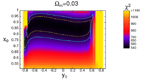
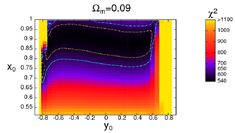
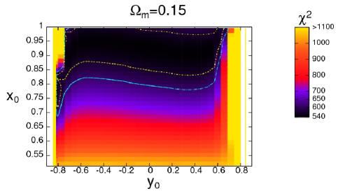
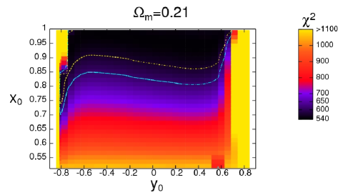
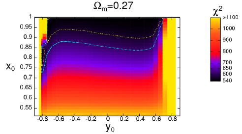
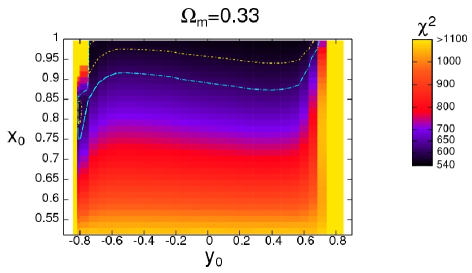
Figure 1: (Color online) The fit of the luminosity distance vs redshift for the parameters $k=0.4$ and $\Omega_{m}=0.03$ (upper left), $0.09$ (upper right), $0.15$ (middle left), $0.21$ (middle right), $0.27$ (lower left), $0.33$ (lower right), in the parameter plane ($y_{0}$, $x_{0}$) in the range $\left|y_{0}\right|\leq 0.845$ where the potential $V$ is well defined. The contours refer to the $68.3\%$ (1$\sigma$) and $95.4\%$ (2$\sigma$) confidence levels. The color code for $\chi^{2}$ is indicated on the vertical stripes. The clear tendency with increasing the dust component is that the parameter $x_{0}$ approaches its maximally allowed value (representing $\dot{T}_{0}=0$). Higher values of $\Omega_{m}$ render the fit with the supernovae outside the 1$\sigma$ region.

In subsection IVA we investigate the compatibility with SNIa data of this dark energy model in the presence of dustlike matter. We use the Union2 SNIa data set Union2 . We show that the model fits the SNIa data well also in the presence of dustlike matter.

In subsection IVB we investigate the future evolution numerically for those trajectories which run into the soft singularity at time $t_{S_{1}}$. We give specifically the time intervals measured from today for the following events: $t_{dec}$ when the cosmic expansion becomes decelerated; $t_{\ast}$ corresponding to the tachyon-pseudotachyon transformation (crossing the corner of the rectangle in the phase portrait of the model); $t_{S_{1}}$ when the first soft singularity is reached; $t_{turn}$ corresponding to the turning point when the universe starts contracting; $t_{S_{2}}$ when the second soft singularity is reached; and finally the time $t_{BC}$ of the Big Crunch.

IV.1 Test with supernovae data

The tachyon field violates the strong energy condition when $\dot{T}^{2}<1$, as required by a dark energy candidate. For a reasonable fit with supernova data we assume $\dot{T}^{2}<1$. In the regime where $a$ varies monotonically with time it may be convenient to replace the cosmological time with a monotonic function of the scale factor as a new independent variable. We choose the redshift $1+z=a_{0}/a$ as a new independent variable (here and henceforth the subscript $0$ refers to the value of the respective quantities at the present epoch).

The model depends on the parameters $k$ and $\Lambda$. For given values of these parameters the possible solutions depend on the quantity of dust and on the initial conditions $y_{0},\dot{T}_{0}$ for the tachyon field. However, the Friedmann equation implies the following constraint

$$\dot{T}_{0}=\pm\sqrt{1-\frac{\ \Omega_{\Lambda,0}^{2}\left[1-\left(1+k\right)y_{0}^{2}\right]}{\left(1-\Omega_{m,0}\right)^{2}\left(1-y_{0}^{2}\right)^{2}}},$$ (53)

where (remembering our convention $8\pi G/3=1$)

$$\,\Omega_{\Lambda,0}=\frac{\Lambda}{H_{0}^{2}},~{}\Omega_{m,0}=\frac{\rho_{m,0}}{H_{0}^{2}},$$ (54)

showing that $\Lambda$ is determined by the values of the other parameters. In what follows we fix $k=0.4$ and vary $\Omega_{m,0}$ through the values $\{0.03$, $0.09$, $0.15$, $0.21$, $0.27$, $0.33\}$. As in paper tach1 we avoid the double coverage of the parameter space (the model has a symmetry given by Eq. (19)) by replacing $\dot{T}_{0}$ tach1 with the new variable:

$$x_{0}=\frac{1}{1+\dot{T}_{0}^{2}}.$$ (55)

The initial conditions $x_{0}$ and $y_{0}$ vary inside the rectangle $\frac{1}{2}\leq x_{0}\leq 1,|y_{0}|\leq 0.845$. Finally, we introduce the luminosity distance $d_{L}$ whose evolution is given by

$$\frac{d}{dz}\left(\frac{d_{L}}{1+z}\right)=\frac{1}{H}.$$ (56)

Fitting to the supernovae data involves a $\chi^{2}$-test, as described in Refs. DicusRepko , tach1 . In Fig 1 we show the $\chi^{2}$ values in the parameter plane of the initial conditions $\left(y_{0},x_{0}\right)$. The contours correspond to the 1 $\sigma$, respectively 2$\sigma$, confidence levels with $\chi^{2}=570.34$ and $\chi^{2}=612.33$, respectively.

IV.2 Future evolution

As in the preceding papers tach1 ; tach2 we study numerically the future evolution of the universe starting with initial conditions compatible with SNIa data. However, our task now is technically more complicated due to the presence of dust. As a matter of fact, we shall have to consider five different regimes, where different systems of dynamical equations are used and we should provide four accurate matching between these evolutions. First, the universe starts its evolution at some point in the rectangle on the phase space of Fig. 4 of tach0 . Here the field $T$ satisfies the equation of motion (12) and the right-hand side of the first Friedmann equation includes the contribution of dust (27) and of the tachyon field (10). After the crossing of the corner (at $t_{\ast}$), the tachyon field transforms into a pseudotachyon field with equation of motion (26) and energy density (24). This is the second regime. The third regime enters into action after the first crossing of the soft singularity (at $t_{S_{1}}$), when the pseudotachyon transforms itself into a quasitachyon with equation of motion (45) and energy density (46). After the passing of the point of maximal expansion of the universe (at $t_{turn}$) we enter into the fourth regime when the universe starts contracting. After the second soft singularity crossing (at $t_{S_{2}}$) we have the fifth regime, where the quasitachyon converts itself again into a pseudotachyon. Finally, the universe ends in a Big Crunch (at $t_{BC}$). The corresponding times are shown in Table 1 for $\Omega_{m,0}=0.03$ and in Table 2 for $\Omega_{m,0}=0.27$ .

These times have been computed assuming for $H_{0}$ the value $70$ km s^-1 Mps ^-1. It is known that there is a certain discrepancy between the value of the Hubble parameter arising indirectly from the cosmic microwave background and baryon acoustic oscillations Planck , and the one more directly obtained from local measurements of the relation between redshifts and distances to sources Riess (for a recent analysis of this problem see variance ). The former gives $H_{0}^{CMB}=67.89\pm 0.77$ km s^-1 Mps^-1, while the latter gives $H_{0}^{local}=73.8\pm 2.4$ km s^-1 Mps^-1. Nevertheless, the precise value of $H_{0}$ is not so important for our study, hence, we have taken an intermediate value.

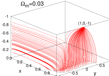
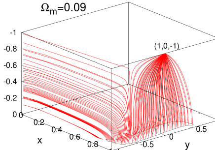
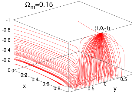
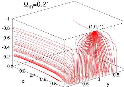
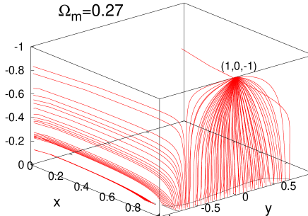
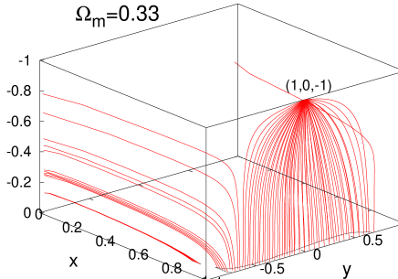
Figure 2: (Color online) The future evolution of those universes, which are in a $68.3\%$ confidence level fit with the supernova data. The 1$\sigma$ contours (black lines in the $z=0$ plane) are from Fig 1 (the parameter plane $\left(y_{0},x_{0}\right)$ is the $z=0$ plane here). The sequence of figures and the values of $\Omega_{m,0}$ are the same as on Fig. 1. The point $(1,0,-1)$ is the de Sitter final state.

Table 1: Key times in the evolution of tachyon universes for $k=0.4$ and $\Omega_{m,0}=0.03$ are given. The first two columns give initial values $x_{0}$, $y_{0}$ in agreement with supernovae data at the 1$\sigma$ confidence level. Remaining columns starting from left give the successive times (measured from the present time): $t_{dec}$ when the expansion becomes decelerated, the tachyonic tansition time $t_{\ast}$, the first soft singularity crossing time $t_{S_{1}}$, the turning point $t_{turn}$, the second soft singularity crossing time $t_{S_{2}}$ and finally the Big Crunch time $t_{BC}$. Times are given in $10^{9}yrs$ unit and calculated assuming $H_{0}=70$ km s^-1 Mpc^-1.

$y_{0}$	$x_{0}$	$t_{dec}$	$t_{\ast}$	$t_{S_{1}}$	$t_{turn}$	$t_{S_{2}}$	$t_{BC}$
$-0.80$	$0.725$	$0.60658$	$0.89098$	$1.71951$	$1.71980$	$1.72032$	$2.01708$
$-0.80$	$0.755$	$0.65334$	$0.90487$	$1.69670$	$1.69698$	$1.69747$	$1.99019$
$-0.75$	$0.875$	$2.24655$	$2.48989$	$3.29101$	$3.29119$	$3.29153$	$3.59233$
$-0.65$	$0.875$	$6.64484$	$6.87894$	$7.69232$	$7.69237$	$7.69247$	$8.00317$
$-0.60$	$0.845$	$9.29396$	$9.52553$	$10.34418$	$10.34420$	$10.34425$	$10.65883$

Table 2: Same as in Table 1 for $\Omega_{m,0}=0.27$.

$y_{0}$	$x_{0}$	$t_{dec}$	$t_{\ast}$	$t_{S_{1}}$	$t_{turn}$	$t_{S_{2}}$	$t_{BC}$
$-0.80$	$0.770$	$0.65390$	$1.05684$	$1.90378$	$1.91751$	$1.93727$	$2.24682$
$-0.75$	$0.875$	$2.53938$	$2.90537$	$3.78730$	$3.79630$	$3.80968$	$4.13589$
$-0.75$	$0.950$	$3.11633$	$3.43361$	$4.28179$	$4.28892$	$4.29969$	$4.62210$
$-0.70$	$0.965$	$6.64092$	$6.92923$	$7.81031$	$7.81302$	$7.81738$	$8.15389$
$-0.65$	$0.995$	$21.07994$	$21.33077$	$22.22677$	$22.22681$	$22.22689$	$22.57314$

Now we can turn to the analysis of the Tables I and II. In Table 1 different times measured from today are given for a low amount of dust $\Omega_{m,0}=0.03$ and in Table 2 for $\Omega_{m,0}=0.27$. So we see the effect of the addition of dust in a systematic way. Three comments are in order here.

First, the time interval $t_{\ast}$ between today and the first transition into the pseudotachyon varies considerably within the set of trajectories compatible with the supernovae data. Namely, it varies from 0.9 to 9.5 billion years for $\Omega_{m,0}=0.03$ and from 1 to 21 billion years $\Omega_{m,0}=0.27$. Second, the time intervals between $t_{\ast}$ and the Big Crunch time $t_{BC}$ are practically constant (about 1.1 billion years for the first case and about 1.2 billion years for the second case). A similar property was found in the model without dust tach2 . Third, the time interval between the two soft singularity crossings $t_{S_{2}}-t_{S_{1}}$ decreases strongly (from 810 thousand years to 70 thousand years for the first case and from 0.03 to 0.0002 billion years for the second case) when the value of $t_{\ast}$ increases. This can be ascribed to the fact that the density of dust, at the moment of the first soft singularity crossing $t_{S_{1}}$, for the universes with high values of $t_{\ast}$ is greatly reduced compared to those with small values of $t_{\ast}$. Indeed, in the absence of dust the two values $t_{S_{1}}$ and $t_{S_{2}}$ coincide and we have a unique Big Brake singularity.

On Figure 2 the evolutions are shown in the three-dimensional coordinate space $x,y,z$ for six different values of $\Omega_{m,0}$. For the trajectories ending in a de Sitter space, the final point has coordinates $(1,0,-1)$. For other trajectories we present only the evolutions until the first soft singularity crossing. Generally, the sets of initial conditions, compatible with the supernovae data (the regions in the plane $(x,y)$ at $z=0$) decrease as the quantity of dust increases and vanish for $\Omega_{m,0}>0.33$. Also, as $\Omega_{m,0}$ increases, the number of trajectories going to a soft singularity is decreasing compared to those ending in a de Sitter space.

This work is done with the spatially-flat paradigm in mind. However, as this model is constrained using SNIa data, it is interesting to relax the assumption of flatness in this case and to consider also non-flat universes with a spatial curvature allowed by observations. Indeed in a spatially closed universe the curvature and matter terms in the Friedmann equation could cancel each other at some (negative) redshift $z_{curv}$

$$1+z_{curv}=\frac{|\Omega_{k,0}|}{\Omega_{m,0}}~{}.$$ (57)

The quantity $\Omega_{k,0}$ is strongly constrained by observations, $-0.0065\leq\Omega_{k,0}\leq 0.0012$ (95% C.L.) with central value $\Omega_{k,0}=-0.0027$ WMAP12 . Hence a slightly spatially closed universe is favoured.

Of course the tachyon, like any scalar field model and in sharp contrast to the anti-Chaplygin gas, does not have a barotropic equation of state. Therefore the amount of expansion needed to reach the soft singularity depends on the initial conditions. It is quite clear however that for models studied here we will have $|z_{S_{1}}|<|z_{curv}|$. Hence the kind of problem considered in this paper, and the mechanism suggested in order to cross the soft singularity, will remain even in the presence of a tiny curvature. But we conjecture that peculiar initial conditions do exist for which this is no longer the case.

V Concluding Remarks

Soft cosmological singularities known since the 1980s Tipler2 , have been attracting growing attention during the last few years soft . In this paper we have continued the investigation of particular cosmological models based on tachyon fields or perfect fluids (introduced in paper tach0 ), for which soft singularities arise in a natural way. The main result of our investigation is the description of a smooth crossing of soft singularities, arising in models with anti-Chaplygin gas or of a particular tachyon field in the presence of dust. Such a crossing is accompanied by certain transformations of matter properties, embodied in a change either of equation of state or of Lagrangian.

The interesting feature of the tachyon model is that there exist cosmological evolutions whose past is compatible with the supernova data and whose future reveals “exotic phase transitions” which are described here in detail. We have performed a detailed numerical analysis of these evolutions.

All our studies, both theoretical and numerical, were performed assuming a a spatially-flat universe. Next interesting step for the study of dark energy models possessing soft future singularities is the inclusion of spatially closed universes. Indeed, observations do allow for a tiny spatial curvature, a positive curvature being slightly preferred. While a tiny viable curvature will not change the situation for most models studied in this paper, a larger number of situations can arise in the presence of spatial curvature for the tachyon models because of their rich dynamics. Indeed, if the universe reaches the point of maximal expansion before occurence of the soft future singularity, the latter will not occur at all. In the case of our tachyon model this can happen for specific initial conditions. If for some peculiar initial conditions the turning point and the soft singularity coincide the latter retains its character of a Big Brake singularity. (In another dark energy model, based on a standard scalar field, such an interplay between turning point and the encounter with a soft singularity was considered in manti ). For a comprehensive investigation of these situations a more detailed study is required, both theoretical and numerical and this is left for future work future . In contrast, the possible situations in the case of the anti-Chaplygin gas are more straightforward.

Another interesting direction of development of the present work is the consideration of cosmological perturbations and their possible influence on the structure of sudden singularities and on the conditions of their crossing. To our knowledge no systematic study of this kind appeared yet in the literature.

References

- (1) Z. Keresztes, L. Á. Gergely, and A. Yu. Kamenshchik, Phys. Rev. D 86, 063522 (2012).
- (2) V. Gorini, A.Yu. Kamenshchik, U. Moschella, and V. Pasquier, Phys. Rev. D 69, 123512 (2004).
- (3) L. Fernández-Jambrina and R. Lazkoz, Phys. Rev. D 70, 121503 (2004).
- (4) Z. Keresztes, L.Á. Gergely, A.Yu. Kamenshchik, V. Gorini, and D. Polarski, Phys. Rev. D 82, 123534 (2010).
- (5) F. J. Tipler, Phys. Lett. A 64, 8 (1977).
- (6) A. Królak, Class. Quantum Grav. 3, 267 (1986).
- (7) A.Yu. Kamenshchik, U. Moschella and V. Pasquier, Phys. Lett. B 511, 265 (2001).
- (8) J.C. Fabris, S.V.B. Goncalves and P.E. de Souza, Gen. Relativ. Grav. 34, 53 (2002); N. Bilic, G.B. Tupler and R.D. Viollier, Phys. Lett. B 535, 17 (2002); M.C. Bento, O. Bertolami and A.A. Sen, Phys. Rev. D 66, 043507 (2002), V. Gorini, A.Yu. Kamenshchik and U. Moschella, Phys. Rev. D 67, 063509 (2003).
- (9) B. Carter, Phys. Lett. B 224, 61 (1989); A. Vilenkin, Phys. Rev. D 41, 3038 (1990).
- (10) A. Sen, J. High Energy Phys. 04, 048 (2002).
- (11) Z. Keresztes, L. Á. Gergely, V. Gorini, U. Moschella, and A.Yu. Kamenshchik, Phys. Rev. D 79, 083504 (2009).
- (12) A.A. Andrianov, F. Cannata and A.Yu. Kamenshchik, Phys. Rev. D 72, 043531 (2005), F. Cannata and A.Yu. Kamenshchik, Int. J. Mod. Phys. D 16, 1683 (2007).
- (13) I.M. Khalatnikov, Phys. Lett. B 563, 123 (2003).
- (14) A. Frolov, L.A. Kofman and A.A. Starobinsky, Phys. Lett. B 545, 8 (2002).
- (15) R. Amanullah et al., Astrophys. J. 716, 712 (2010).
- (16) D. A. Dicus and W. W. Repko, Phys. Rev. D 70, 083527 (2004).
- (17) P. Ade et al/ (Planck Collaboration), arXiv: 1303.5076 [astro-ph.CO].
- (18) A.G. Riess, L. Macri, S. Casertano, H. Lampeitl, H.C. Ferguson, et al., Astrophys. J. 730, 119 (2011).
- (19) V. Marra, L. Amendola, I. Sawicki and W. Valkenburg, Phys. Rev. Lett. 110, 241305 (2013).
- (20) J.D. Barrow, G.J. Galloway and F.J. Tipler, Mon. Not. R. Astron. Soc. 223, 835 (1986).
- (21) J.D. Barrow, Class. Quantum Garv. 21, L79 (2004); Class. Quantum Garv. 21, 5619 (2004); M.P. Dabrowski, T. Denkiewicz and M.A. Hendry, Phys. Rev. D 75, 123524 (2007); Yu. Shtanov and V. Sahni, Class. Quantum Grav. 19, L101 (2002).
- (22) G. Hinshaw et al., arXiv:1212.5226
- (23) A.Yu. Kamenshchik and S. Manti, Phys. Rev. D 85, 123518 (2012).
- (24) Zs. Gyöngyösi, Z. Keresztes, L.Á. Gergely, A.Yu. Kamenshchik, V. Gorini, and D. Polarski (to be published).