Formation of stripes and slabs near the ferromagnetic transition

Abstract

We consider Ising models in $d=2$ and $d=3$ dimensions with nearest neighbor ferromagnetic and long-range antiferromagnetic interactions, the latter decaying as (distance)^-p, $p>2d$, at large distances. If the strength $J$ of the ferromagnetic interaction is larger than a critical value $J_{c}$, then the ground state is homogeneous. It has been conjectured that when $J$ is smaller than but close to $J_{c}$ the ground state is periodic and striped, with stripes of constant width $h=h(J)$, and $h\to\infty$ as $J\to J_{c}^{-}$. (In $d=3$ stripes mean slabs, not columns.) Here we rigorously prove that, if we normalize the energy in such a way that the energy of the homogeneous state is zero, then the ratio $e_{0}(J)/e_{\rm S}(J)$ tends to 1 as $J\to J_{c}^{-}$, with $e_{\rm S}(J)$ being the energy per site of the optimal periodic striped/slabbed state and $e_{0}(J)$ the actual ground state energy per site of the system. Our proof comes with explicit bounds on the difference $e_{0}(J)-e_{\rm S}(J)$ at small but finite $J_{c}-J$, and also shows that in this parameter range the ground state is striped/slabbed in a certain sense: namely, if one looks at a randomly chosen window, of suitable size $\ell$ (very large compared to the optimal stripe size $h(J)$), one finds a striped/slabbed state with high probability.

1 Introduction and main results

We consider Ising models in two and three dimensions on the square lattice with the formal Hamiltonian

$$H=-J\sum_{{\left\langle{\bf x},{\bf y}\right\rangle}}(\sigma_{\bf x}\sigma_{\bf y}-1)+\sum_{\{{\bf x},{\bf y}\}}\frac{(\sigma_{\bf x}\sigma_{\bf y}-1)}{|{\bf x}-{\bf y}|^{p}}$$ (1.1)

where the first sum ranges over nearest neighbor pairs in $\mathbb{Z}^{d}$, $d=2,3$, the second over pairs of distinct sites in $\mathbb{Z}^{d}$, and the exponent $p$ is chosen to satisfy $p>2d$, for reasons that will become clear below. For more general values of $p$, this model is used to describe the effects of frustration induced in thin magnetic films by the presence of dipolar interactions ($p=3$) or in two-dimensional charged systems by the presence of an unscreened Coulomb interaction ($p=1$) [1, 2, 4, 5, 6, 7, 8, 9, 10, 19, 21, 22, 23, 24, 25, 26, 27, 31, 32], see also [3, 12, 13, 14, 15, 16, 17, 18] for a more detailed introduction to the subject, as well as for previous rigorous results. The competition between short range ferromagnetic and long-range antiferromagnetic interaction is believed to be responsible for the emergence of non-trivial “mesoscopic patterns” in the ground and low-temperature states of the system. Let us be more specific. As proved in [17], if $J>J_{c}$, with

$$J_{c}:=\sum_{y_{1}>0,\ {\bf y}^{\perp}\in\mathbb{Z}^{d-1}}\frac{y_{1}}{(y_{1}^{2}+|{\bf y}^{\perp}|^{2})^{p/2}}\;,$$ (1.2)

then there are exactly two ground states, $\sigma_{\bf x}\equiv+1$ $\forall{\bf x}\in\mathbb{Z}^{d}$, and $\sigma_{\bf x}\equiv-1$ $\forall{\bf x}\in\mathbb{Z}^{d}$. Note that $J_{c}$ is the value of the ferromagnetic coupling such that the energy of a straight domain wall configuration, i.e., a configuration consisting of half the spins minus (those at the left of a vertical straight plane) and half the spins plus (those at the right of the same plane), vanishes. If $J\lesssim J_{c}$, the ground state is certainly non-homogeneous. There is evidence that the transition to the ferromagnetic phase as $J\to J_{c}^{-}$ takes place via a series of “microemulsion phases” characterized by phase separation on a mesoscopic scale that is large compared to the lattice and small compared to the scale of the whole sample; see e.g. [20, 28, 29, 30] for a discussion of this phenomenon in the case of Coulomb ($p=1$) and dipolar ($p=3$) interactions. More precisely, at zero temperature, the transition to the ferromagnetic state is expected to take place via a sequence of transitions between periodic striped or slabbed states, depending on dimensionality, consisting of stripes/slabs (either vertical or horizontal) all of constant width $h(J)$ and of alternating sign. If we denote by $e_{\rm s}(h)$ the energy per site in the thermodynamic limit of periodic striped/slabbed configurations consisting of stripes/slabs all of size $h$, the optimal stripe/slabs width $h(J)$ can be obtained by minimizing $e_{\rm s}(h)$ over $h\in\mathbb{N}$, and turns out to be of the order $(J_{c}-J)^{-\frac{1}{p-d-1}}$. Let us denote by $e_{\rm S}(J):=e_{\rm s}(h(J))$ the optimal striped/slabbed energy per site and by $e_{0}(J)$ the actual ground state energy per site in the thermodynamic limit. Our main result can be summarized in the following theorem:

Theorem 1.

As to $J\to J_{c}$ from below, we have

$$\lim_{J\to J_{c}^{-}}\frac{e_{0}(J)}{e_{\rm S}(J)}=1\;.$$ (1.3)

Eq. (1.3) is a strong indication of the conjectured periodic striped/slabbed structure of the ground state. The proof of Eq. (1.3) comes with explicit bounds on the speed of convergence to the limit, namely

$$\frac{e_{0}(J)}{e_{\rm S}(J)}=1+O\big{(}(J_{c}-J)^{\frac{p-2d}{(d-1)(p-d-1)}}\big{)}\;.$$ (1.4)

It also comes with explicit bounds on the energy cost of the “corners”. This notion was introduced in [17] for the two-dimensional case; every time that a domain wall bends by 90^o, hence creating a corner (or an edge corner, as we call it, in three-dimensions: this is an edge where two plaquettes come together at 90^o), we pay a positive energy cost, at least in the case that the corner density is sufficiently high. Combining this remark with our a priori bounds on the ground state energy, we find that the ground state has a density of corners that is smaller than $(J_{c}-J)^{d/(d-1)}$: therefore, if we look in a random window of proper side $\ell^{\prime}$ (much larger than the optimal stripe/slab width $h(J)\sim(J_{c}-J)^{-\frac{1}{p-d-1}}$, and much smaller than the typical separation between corners $\sim(J_{c}-J)^{-1/(d-1)}$), the ground state restricted to such a window is striped/slabbed, with stripes/slabs of width close to the optimal size $h(J)$. Our proof presumably adapts to any dimension, e.g., $d=10,11$ or $26$, and the interested reader can extend the arguments in Appendix D if desired.

The logic of the proof goes as follows. We first derive an alternative representation of the energy in terms of droplet self-energies and droplet-droplet interactions. Next, for the purpose of a lower bound, we localize the energy into squares/cubes of side $\ell$ (to be optimized over), and we show that the localized self-energy of every droplet with at least one corner along its boundary is positive; therefore, we can eliminate all such droplets, after which we are left only with striped/slabbed droplets. Finally, reflection positivity shows that the optimal striped/slabbed configuration is periodic.

2 Droplets and self-energies

Defining $\tau:=2(J-J_{c})$, the optimal periodic striped energy per site has the form:

$$e_{\rm S}(J)=-C_{s}(\tau)|\tau|^{(p-d)/(p-d-1)},$$ (2.1)

with $C_{\rm s}(\tau)=C_{\rm s}(0)+O(|\tau|^{2/(p-d-1)})$ asymptotically for $\tau\to 0^{-}$, for a suitable $C_{\rm s}(0)>0$. This result follows from the explicit minimization of $e_{\rm s}(h)$, see Appendix A, and can also be understood in terms of a balance between “line” or “plane” energies and line-line or plane-plane interactions, see [17, Section II]. We note that the computation in Appendix A also shows that the optimal stripe/slab width is

$$h^{*}={\rm argmin}\,e_{\rm s}(h)=\tilde{C}_{\rm s}(\tau)|\tau|^{-1/(p-d-1)}\;,$$ (2.2)

with $\tilde{C}_{\rm s}(\tau)=\tilde{C}_{\rm s}(0)+O(|\tau|^{2/(p-d-1)})$ asymptotically for $\tau\to 0^{-}$, for a suitable $\tilde{C}_{\rm s}(0)>0$. Of course, $e_{0}(J)\leq e_{\rm S}(J)$. Our purpose is to get a comparable lower bound, of the form

$$e_{0}(J)\geq-C_{\rm s}(0)|\tau|^{(p-d)/(p-d-1)}\,\big{(}1+O(|\tau|^{\beta})\big{)}\;,$$ (2.3)

for some positive $\beta$. The strategy borrows some ideas from those in [17, Appendix A].

From now on, for the purpose of simplicity of exposition, we restrict ourselves to two dimensions. We shall explain how to adapt the proof to three dimensions in Appendix D. We need to recall the definitions of contours and droplets. Let us first define the finite volume Hamiltonian for our system:

$$H_{\Lambda}({\underline{\sigma}}_{\Lambda})=-J\sum_{\begin{subarray}{c}{\left\langle{\bf x},{\bf y}\right\rangle}:\\ {\bf x},{\bf y}\in\Lambda\end{subarray}}(\sigma_{\bf x}\sigma_{\bf y}-1)+\sum_{\begin{subarray}{c}\{{\bf x},{\bf y}\}:\\ {\bf x},{\bf y}\in\Lambda\end{subarray}}\frac{(\sigma_{\bf x}\sigma_{\bf y}-1)}{|{\bf x}-{\bf y}|^{p}}+\mathcal{B}_{\Lambda}({\underline{\sigma}}_{\Lambda}|{\underline{\sigma}}^{*})\;.$$ (2.4)

Here $\Lambda\subset\mathbb{Z}^{2}$ is a square box, ${\underline{\sigma}}_{\Lambda}=\{\sigma_{\bf x}\}_{{\bf x}\in\Lambda}\in\{\pm 1\}^{\Lambda}$ is the spin configuration in $\Lambda$, ${\underline{\sigma}}^{*}=\{\sigma_{\bf x}^{*}\}_{{\bf x}\in\mathbb{Z}^{2}}\in\{\pm 1\}^{\mathbb{Z}^{2}}$ is a boundary condition and

$$\mathcal{B}_{\Lambda}({\underline{\sigma}}_{\Lambda}|{\underline{\sigma}}^{*})=-J\sum_{\begin{subarray}{c}{\bf x}\in\Lambda,\ {\bf y}\in\Lambda^{c}:\\ |{\bf x}-{\bf y}|=1\end{subarray}}(\sigma_{\bf x}\sigma_{\bf y}-1)+\sum_{{{\bf x}\in\Lambda,\ {\bf y}\in\Lambda^{c}}}\frac{(\sigma_{\bf x}\sigma_{\bf y}-1)}{|{\bf x}-{\bf y}|^{p}}\;.$$ (2.5)

In the discussion below, we shall consider $+$ boundary conditions: this means that $\underline{\sigma}^{*}=\{+1\}^{\mathbb{Z}^{2}}$.

Given ${\underline{\sigma}}_{\Lambda}$, we define $\Delta$ to be the set of sites at which $\sigma_{\bf x}=-1$, i.e., $\Delta=\{{\bf x}\in\Lambda\,:\,\sigma_{\bf x}=-1\}$. Around each ${\bf x}\in\Delta$ we draw the $4$ sides of the unit square centered at ${\bf x}$ and suppress the sides that occur twice: in this way we obtain a closed polygon $\Gamma(\Delta)$ which can be thought of as the boundary of $\Delta$. Each side of $\Gamma(\Delta)$ separates a point ${\bf x}\in\Delta$ from a point ${\bf y}\not\in\Delta$. At every vertex of $\Gamma(\Delta)\cap(\mathbb{Z}^{2})^{*}$, with $(\mathbb{Z}^{2})^{*}$ the dual lattice of $\mathbb{Z}^{2}$, there can be either 2 or 4 sides meeting. In the case of 4 sides, we deform the polygon slightly by “chopping off” the edge from the squares containing a $-$ spin. See Figure 1.

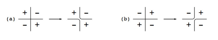
Figure 1: In the case that 4 sides of the closed polygon $\Gamma(\Delta)$ meet at a vertex $v$, we slightly deform $\Gamma(\Delta)$ so that the two squares containing a $-$ spin become disconnected from the vertex itself. Case (a) represents the situation where the minus spins are located at NE and SW of $v$, before and after the “chopping”. Case (b) represents the situation where the minus spins are located at NW and SE of $v$, before and after the “chopping”.

When this is done $\Gamma(\Delta)$ splits into disconnected polygons $\Gamma_{1},\ldots,\Gamma_{r}$ which are called contours. Note that, because of the choice of $+$ boundary conditions, all the contours are closed. The definition of contours naturally induces a notion of connectedness for the spins in $\Delta$: given ${\bf x},{\bf y}\in\Delta$ we shall say that ${\bf x}$ and ${\bf y}$ are connected if and only if there exists a sequence $({\bf x}={\bf x}_{0},{\bf x}_{1},\ldots,{\bf x}_{n}={\bf y})$ such that ${\bf x}_{m},{\bf x}_{m+1}$, $m=0,\ldots,n-1$, are nearest neighbors and none of the bonds $({\bf x}_{m},{\bf x}_{m+1})$ crosses $\Gamma(\Delta)$. The maximal connected components $\delta_{i}$ of $\Delta$ will be called droplets and the set of droplets of $\Delta$ will be denoted by ${\cal D}(\Delta)=\{\delta_{1},\ldots,\delta_{s}\}$. Note that the boundaries $\Gamma(\delta_{i})$ of the droplets $\delta_{i}\in{\cal D}(\Delta)$ are all distinct subsets of $\Gamma(\Delta)$ with the property: $\cup_{i=1}^{s}\Gamma(\delta_{i})=\Gamma(\Delta)$.

Given the definitions above, let us rewrite the energy $H_{\Lambda}({\underline{\sigma}}_{\Lambda})$ of ${\underline{\sigma}}_{\Lambda}$ with + boundary conditions as

$$H_{\Lambda}({\underline{\sigma}}_{\Lambda})=2J\sum_{\Gamma\in\Gamma(\Delta)}|\Gamma|+\sum_{\delta\in{\cal D}(\Delta)}U(\delta)+\sum_{(\delta,\delta^{\prime})}W(\delta,\delta^{\prime})\;,$$ (2.6)

where, if $\delta^{c}=\mathbb{Z}^{2}\setminus\delta$,

$$U(\delta):=-2\sum_{{\bf x}\in\delta}\sum_{{\bf y}\in\delta^{c}}\frac{1}{|{\bf x}-{\bf y}|^{p}}$$ (2.7)

is the self-energy of the droplet $\delta$, which is negative. Moreover, the third sum on the r.h.s. of Eq. (2.6) runs over unordered pairs of distinct droplets, and

$$W(\delta,\delta^{\prime}):=4\sum_{{\bf x}\in\delta}\sum_{{\bf y}\in\delta^{\prime}}\frac{1}{|{\bf x}-{\bf y}|^{p}}$$ (2.8)

is the droplet-droplet interaction, which is positive. Note that the choice of + boundary conditions implies that all the droplets are closed and within $\Lambda$.

Our first goal is to get a lower bound on the droplet’s self-energy, which is suitable for later localization of the energy into small squares of side $\ell$, with $\ell\gg h^{*}$, where $h^{*}$ is the optimal stripe width, see Eq. (2.2). For this purpose, given a droplet $\delta\in{\cal D}(\Delta)$ and the corresponding boundary $\Gamma(\delta)$, we define the notion of “bonds facing each other in $\delta$”, in the following way. Let us suppose for definiteness that $b\in\Gamma(\delta)$ is vertical and that it separates a point ${\bf x}_{b}\in\delta$ on its immediate right from a point ${\bf y}_{b}={\bf x}_{b}-(1,0)\not\in\delta$ on its immediate left. Consider the bond $b^{\prime}\in\Gamma(\delta)$ such that: (i) $b^{\prime}$ is vertical; (ii) $b^{\prime}$ separates a point ${\bf x}_{b^{\prime}}\in\delta$ on its immediate left from a point ${\bf y}_{b^{\prime}}={\bf x}_{b^{\prime}}+(1,0)\not\in\delta$ on its immediate right; (iii) the points ${\bf x}_{b}$ and ${\bf x}_{b^{\prime}}$ are at the same height, i.e., $[{\bf x}_{b}]_{2}=[{\bf x}_{b^{\prime}}]_{2}$, and all the points on the same row between them belong to $\delta$: in other words, ${\bf x}_{b}+(j,0)\in\delta$, for all $j=0,\ldots,[{\bf x}_{b^{\prime}}]_{1}-[{\bf x}_{b}]_{1}$. We shall say that $b^{\prime}$ faces $b$ in $\delta$, and vice versa. An analogous definition is valid for horizontal bonds. Note that in the presence of + boundary conditions all the bonds in $\Gamma(\delta)$ come in pairs $b,b^{\prime}$, facing each other in $\delta$.

In Appendix B we show that the self-energy $U(\delta)$ can be bounded from below as

$$U(\delta)\geq-\sum_{i=1,2}\ \sum_{b\in\Gamma_{i}(\delta)}\ \sum_{{{\bf n}\neq{\bf 0}}}\frac{\min\{|n_{i}|,d_{b}(\delta)\}}{|{\bf n}|^{p}}+2^{1-\frac{p}{2}}N_{c}(\delta)+4\sum_{\{{\bf x},{\bf y}\}\in\mathcal{P}(\delta)}\frac{1}{|{\bf x}-{\bf y}|^{p}}\;,$$ (2.9)

where:

• $\Gamma_{i}(\delta)$ is the subset of $\Gamma(\delta)$ consisting of bonds orthogonal to the $i$-th coordinate direction.

• $d_{b}(\delta)$ is the distance between $b$ and the bond $b^{\prime}$ facing it in $\delta$.

• $N_{c}(\delta)$ is the number of corners of $\Gamma(\delta)$.

• $\mathcal{P}(\delta)$ is the set of unordered pairs of distinct sites in $\delta$ such that both $\mathcal{C}^{hv}_{{\bf x}\to{\bf y}}$ and $\mathcal{C}^{hv}_{{\bf x}\to{\bf y}}$ cross at least two bonds of $\Gamma(\delta)$. Here $\mathcal{C}^{hv}_{{\bf x}\to{\bf y}}$ is the path on the lattice that goes from ${\bf x}$ to ${\bf y}$ consisting of two segments, the first horizontal and the second vertical. Similarly, $\mathcal{C}^{vh}_{{\bf x}\to{\bf y}}$ is the path on the lattice that goes from ${\bf x}$ to ${\bf y}$ consisting of two segments, the first vertical and the second horizontal (note that the two paths can coincide, in the case that $x_{i}=y_{i}$ for some $i\in\{1,2\}$).

The lower bound in Eq. (2.9) is very convenient for localization of the energy into small boxes, as shown explicitly in the next section. Let us remark that, if desired, the first term on the r.h.s. of this inequality can be further bounded from below as

$$-\sum_{i=1,2}\ \sum_{b\in\Gamma_{i}(\delta)}\ \sum_{{{\bf n}\neq{\bf 0}}}\frac{\min\{|n_{i}|,d_{b}(\delta)\}}{|{\bf n}|^{p}}\geq-\sum_{i=1,2}\ \sum_{b\in\Gamma_{i}(\delta)}\ \sum_{{\bf n}\neq{\bf 0}}\frac{|n_{i}|}{|{\bf n}|^{p}}=-2J_{c}|\Gamma(\delta)|\;.$$ (2.10)

3 Localization and minimization

We introduce a partition of the big box $\Lambda$ into squares $Q$ of side $\ell$, to be optimized in the following. Our purpose is to localize the energy into these squares, and to minimize the energy exactly in each small box, thus deriving a lower bound on the global energy of the system. Given a droplet configuration $\mathcal{D}$ and $\delta\in\mathcal{D}$, we say that $b\in\Gamma(\delta)$ belongs to $Q$ if either it belongs to the interior of $Q$, or it belongs to the boundary of $Q$ and separates a site ${\bf x}\in\delta\cap Q$ from a site ${\bf y}\not\in\delta$. Note that with this definition every bond in $\Gamma(\delta)$ belongs to exactly one square $Q$. The set of bonds $b\in\Gamma(\delta)$ belonging to $Q$ will be denoted by $\Gamma_{Q}(\delta)$. The notion that we just introduced induces a partition of $\Gamma(\delta)$ into disjoint pieces assigned to different squares: $\Gamma(\delta)=\cup_{Q}\Gamma_{Q}(\delta)$. Moreover, if $\delta_{Q}=\delta\cap Q$, we define $\bar{\delta}_{Q}^{(1)},\ldots,\bar{\delta}_{Q}^{(m_{Q}(\delta))}$ to be the maximal connected components of $\delta_{Q}$, and $\bar{\Gamma}_{Q}^{(1)},\ldots,\bar{\Gamma}_{Q}^{(m_{Q}(\delta))}$ to be the portions of $\Gamma_{Q}(\delta)$ belonging to the boundary of $\bar{\delta}_{Q}^{(1)},\ldots,\bar{\delta}_{Q}^{(m_{Q}(\delta))}$, respectively. We shall refer to the pair $(\bar{\delta}_{Q}^{(i)},\bar{\Gamma}_{Q}^{(i)})$ as to a bubble in $Q$ originating from $\delta$. We shall indicate by $\bar{\mathcal{B}}_{Q}(\delta)$ the set of bubbles in $Q$ originating from $\delta$, and by $\bar{\mathcal{B}}_{Q}=\cup_{\delta\in\mathcal{D}}\bar{\mathcal{B}}_{Q}(\delta)$ the total set of bubbles in $Q$.

Given $\bar{\beta}=(\bar{\delta},\bar{\Gamma})\in\bar{\mathcal{B}}_{Q}$, note that in general $\bar{\Gamma}$ is a union of disjoint polygonal curves, each of which can be either closed or open. If one of these curves is open, then its endpoints must belong to the boundary of $Q$. Given an endpoint $v$ of an open component of $\bar{\Gamma}$ such that: (1) $v$ is not at a corner of $Q$, (2) the bond $b\in\bar{\Gamma}$ exiting from $v$ belongs to the boundary of $Q$; then we shall say that $\bar{\Gamma}$ has a “boundary corner” at $v$. The corners of $\bar{\Gamma}$ belonging to the interior of $Q$ will be called “bulk corners”. Moreover, we shall denote by $\bar{N}_{c}(\bar{\beta})$ the total number of corners of $\bar{\Gamma}$, i.e., the number of its boundary corners plus the number of its bulk corners. Note that

$$\sum_{Q}\sum_{\bar{\beta}\in\bar{\mathcal{B}}_{Q}(\delta)}\bar{N}_{c}(\bar{\beta})\leq N_{c}(\delta)\;.$$ (3.1)

This is an inequality (rather than an equality), in general, because $\delta$ could have corners located exactly at the corners of the squares $Q$. We now derive a lower bound on the total energy in terms of a sum of local energies involving the bubbles we just introduced. First of all, using Eqs. (2.9) and (3.1), we bound the self-energy $U(\delta)$ from below as

$$U(\delta)\geq\sum_{Q}\Big{\{}\sum_{\bar{\beta}\in\bar{\mathcal{B}}_{Q}(\delta)}U_{Q}(\bar{\beta})+\frac{1}{2}\sum_{\begin{subarray}{c}\bar{\beta},\bar{\beta}^{\prime}\in\bar{\mathcal{B}}_{Q}(\delta)\\ \bar{\beta}\neq\bar{\beta}^{\prime}\end{subarray}}W(\bar{\beta},\bar{\beta}^{\prime})\Big{\}}\;,$$ (3.2)

where the first term on the r.h.s. originates from the first two terms on the r.h.s. of (2.9), while the second originates from the last term on the r.h.s. of (2.9). The functions $U_{Q}$ and $W$ are defined as follows: if $\bar{\beta}=(\bar{\delta},\bar{\Gamma})$, $\bar{\beta}^{\prime}=(\bar{\delta}^{\prime},\bar{\Gamma}^{\prime})$,

$$W(\bar{\beta},\bar{\beta}^{\prime})=4\sum_{\begin{subarray}{c}{\bf x}\in\bar{\delta}\\ {\bf y}\in\bar{\delta}^{\prime}\end{subarray}}\frac{1}{|{\bf x}-{\bf y}|^{p}}\;,$$ (3.3)

while

$$U_{Q}(\bar{\beta})=-\sum_{i=1,2}\ \sum_{b\in\bar{\Gamma}_{i}}\ \sum_{{{\bf n}\neq{\bf 0}}}\frac{\min\{|n_{i}|,d^{Q}_{b}(\bar{\delta})\}}{|{\bf n}|^{p}}+2^{1-\frac{p}{2}}\bar{N}_{c}(\bar{\beta})\;.$$ (3.4)

In the last formula, $\bar{\Gamma}_{i}$ is the subset of $\bar{\Gamma}_{i}$ consisting of bonds orthogonal to the $i$-th coordinate direction, and $d_{b}^{Q}(\bar{\delta})$ is the distance between $b$ and the bond $b^{\prime}\in\Gamma(\delta)$ facing it in $\delta$, if both $b$ and $b^{\prime}$ belong to $\bar{\Gamma}$, otherwise it is infinite. In a similar manner, we can bound the droplet-droplet interaction from below as

$$W(\delta,\delta^{\prime})\geq\sum_{Q}\Big{\{}\sum_{\begin{subarray}{c}\bar{\beta}\in\bar{\mathcal{B}}_{Q}(\delta)\\ \bar{\beta}^{\prime}\in\bar{\mathcal{B}}_{Q}(\delta^{\prime})\end{subarray}}W(\bar{\beta},\bar{\beta}^{\prime})\Big{\}}\;.$$ (3.5)

Inserting Eqs. (3.2)–(3.5) into Eq. (2.6) gives

$$H_{\Lambda}({\underline{\sigma}}_{\Lambda})\geq\sum_{Q}E_{Q}(\bar{\mathcal{B}}_{Q})\;,$$ (3.6)

where

$$E_{Q}(\bar{\mathcal{B}}_{Q})=\sum_{\bar{\beta}=(\bar{\delta},\bar{\Gamma})\in\bar{\mathcal{B}}_{Q}}\big{[}2J|\bar{\Gamma}|+U_{Q}(\bar{\beta})\big{]}+\frac{1}{2}\sum_{\begin{subarray}{c}\bar{\beta},\bar{\beta}^{\prime}\in\bar{\mathcal{B}}_{Q}\\ \bar{\beta}\neq\bar{\beta}^{\prime}\end{subarray}}W(\bar{\beta},\bar{\beta}^{\prime})\,.$$ (3.7)

Now consider a bubble $\bar{\beta}=(\bar{\delta},\bar{\Gamma})$ such that $\bar{N}_{c}(\bar{\beta})>0$, i.e., $\bar{\delta}$ is not a stripe. Proceeding as in Eq. (2.10), we can bound $U_{Q}(\bar{\beta})$ as

$$U_{Q}(\bar{\beta})\geq-2J_{c}|\bar{\Gamma}|+2^{1-\frac{p}{2}}\bar{N}_{c}(\bar{\beta})\;.$$ (3.8)

Therefore,

$$2J|\bar{\Gamma}|+U_{Q}(\bar{\beta})\geq\tau|\bar{\Gamma}|+2^{1-\frac{p}{2}}\bar{N}_{c}(\bar{\beta})\;.$$ (3.9)

Note that, in order for $\bar{\Gamma}$ to be very long, the number of corners must be sufficiently large: in formulae,

$$|\bar{\Gamma}|\leq 2\ell+2\ell\bar{N}_{c}(\bar{\beta})\;.$$ (3.10)

[The reason is: (a) $\bar{\Gamma}$ (which, in general, is a disjoint union of polygonal curves) can have at most two exactly straight lines, and this accounts for the $2\ell$. (b) Associated with each corner is an ell-shaped open curve, completely contained in $Q$, with the corner at the apex of the curve. The length of this curve is at most $2\ell$, and it is clear that the union of all these curves covers the remaining part of $\bar{\Gamma}$. This accounts for the $2\ell\bar{N}_{c}(\bar{\beta})$.]

If, as we are assuming, $\bar{N}_{c}(\bar{\beta})>0$, then $\bar{N}_{c}(\bar{\beta})+1\leq 2\bar{N}_{c}(\bar{\beta})$, so that

$$\bar{N}_{c}(\bar{\beta})\geq\frac{|\bar{\Gamma}|}{4\ell}\;.$$ (3.11)

Inserting this back into Eq. (3.9) gives

$$2J|\bar{\Gamma}|+U_{Q}(\bar{\beta})\geq 2^{1-\frac{p}{2}}\frac{|\bar{\Gamma}|}{4\ell}(1-4\cdot 2^{\frac{p}{2}-1}|\tau|\ell)\;,$$ (3.12)

which is positive as soon as $|\tau|\ell<2^{1-\frac{p}{2}}/4$. Therefore, for $\ell$ shorter than $2^{1-\frac{p}{2}}/(4|\tau|)$, we can decrease the local energy $E_{Q}(\bar{\mathcal{B}}_{Q})$ by erasing all the bubbles with at least one corner. Denoting by $\bar{\mathcal{S}}_{Q}\subseteq\bar{\mathcal{B}}_{Q}$ the subset of $\bar{\mathcal{B}}_{Q}$ consisting of bubbles without corners (i.e., consisting of stripes), this means that, if $\ell<2^{1-\frac{p}{2}}/(4|\tau|)$,

$$E_{Q}(\bar{\mathcal{B}}_{Q})\geq E_{Q}(\bar{\mathcal{S}}_{Q})\;.$$ (3.13)

Let now $\bar{\mathcal{S}}_{Q}=\{\bar{\beta}_{1},\ldots,\bar{\beta}_{m}\}$, and let us assume without loss of generality (w.l.o.g.) that the stripes $\bar{\beta}_{i}=(\bar{\delta}_{i},\bar{\Gamma}_{i})$, $i=1,\ldots,m$, are vertical, and are numbered in a way compatible with their order, from left to right. Let us also assume w.l.o.g. that $Q=[1,\ell]^{2}\cap\mathbb{Z}^{2}$. If $m=1$ and $\bar{\beta}_{1}=(Q,\emptyset)$, then $E_{Q}(\bar{\mathcal{S}}_{Q})=0$. Let us then assume that $\bar{\Gamma}_{1}\neq\emptyset$. Note that the contours $\bar{\Gamma}_{i}$ consist of two vertical parallel lines, for all $2\leq i\leq m-1$. If $i=1$, the contour $\bar{\Gamma}_{1}$ can either consist of one or two vertical parallel lines; in the first case, $\bar{\delta}_{1}=[1,y_{1}]\times[1,\ell]\cap\mathbb{Z}^{2}$ for some integer $1\leq i_{1}\leq\ell$, $\Gamma_{1}$ is the vertical line located at the horizontal coordinate $y_{1}+\frac{1}{2}$, and we shall say that $Q$ has $-$ boundary conditions on the left; in the second case, $\bar{\delta}_{1}=[y_{0},y_{1}]\times[1,\ell]\cap\mathbb{Z}^{2}$ for some integers $1\leq y_{0}<y_{1}\leq\ell$, $\Gamma_{1}$ is the pair of vertical lines located at the horizontal coordinates $y_{0}-\frac{1}{2},y_{1}+\frac{1}{2}$, and we shall say that $Q$ has $+$ boundary conditions on the left. Similar definitions are valid for $\bar{\Gamma}_{m}$ and for the boundary conditions on the right. Note that we can always reduce ourselves to the case where both the left and right boundary conditions are $+$, up to an error term that is negligible provided that $\ell\gg h^{*}$. In fact, suppose that the boundary conditions on the left (say) are $-$: then we can change them to $+$ by erasing the bubble $\bar{\beta}_{1}$, thus increasing the energy by at most $|\tau|\ell$. This error term is much smaller than $\ell^{2}e_{\rm stripes}(J)\simeq\ell^{2}|\tau|^{(p-2)/(p-3)}$ if $\ell\gg h^{*}$. Calling $\widetilde{\mathcal{S}}_{Q}\subseteq\bar{\mathcal{S}}_{Q}$ the set of stripes obtained from $\bar{\mathcal{S}}_{Q}$ after the possible erasing of $\bar{\beta}_{1}$ and $\bar{\beta}_{m}$, we then have

$$E_{Q}(\bar{\mathcal{S}}_{Q})\geq E_{Q}(\widetilde{\mathcal{S}}_{Q})+2\tau\ell\;.$$ (3.14)

By construction, $\widetilde{\mathcal{S}}_{Q}$ consists of $k$ vertical stripes, with $k\in\{m-2,m-1,m\}$, whose contours are located at the horizontal coordinates $\frac{1}{2}\leq x_{1}<x_{2}<\cdots<x_{2k}\leq\ell+\frac{1}{2}$. We define $h_{i}=x_{i+1}-x_{i}$, with $i=1,\ldots,2k-1$. At this point we can utilize the reflection positivity of the kernel $|{\bf x}-{\bf y}|^{-p}$ (see [11, 17]), which leads to the chessboard estimate proved in [12, 13, 15]. This estimate yields the inequality (see Appendix C for details)

$$E_{Q}(\widetilde{\mathcal{S}}_{Q})\geq\ell\sum_{i=1}^{2k-1}h_{i}\big{[}e_{\rm s}(h_{i})-Ch_{i}^{3-p}\ell^{-1}\big{]}+\tau\ell-C\ell^{4-p}\;,$$ (3.15)

where $e_{\rm s}(h)$ is the specific energy of the periodic striped configuration with stripes all of size $h$, defined in the introduction, and $C>0$ is a suitable constant. In order to get a lower bound on the r.h.s. of (3.14), we can minimize the expression in square brackets over $h_{i}\leq\ell$:

$$\min_{h_{i}\leq\ell}\big{[}e_{\rm s}(h_{i})-Ch_{i}^{3-p}\ell^{-1}\big{]}=e_{\rm stripes}(J)\big{(}1+({\rm const.})\ell^{-1}|\tau|^{-1/(p-3)})\big{)}\;,$$ (3.16)

which follows from the explicit expression of $e_{\rm s}(h)$ computed in Appendix A, provided that $\ell\gg h^{*}$. Inserting (3.16) into (3.15), and using the fact that $\sum_{i}h_{i}\leq\ell$, we get

$$E_{Q}(\widetilde{\mathcal{S}}_{Q})\geq\ell^{2}e_{\rm S}(J)\big{(}1+({\rm const.})\ell^{-1}|\tau|^{-1/(p-3)})+\tau\ell-C\ell^{4-p}\;,$$ (3.17)

where $e_{\rm S}(J)=-C_{s}(\tau)|\tau|^{(p-2)/(p-3)}$ is the optimal striped energy per site in the thermodynamic limit. Moreover, the minimum in the first line of the last equation is attained at $\bar{h}(\ell)=h^{*}(1+O(h^{*}/\ell))$ with $h^{*}$ given by Eq. (2.2).

Putting things together, we find that, for $\ell<2^{1-\frac{p}{2}}/(4|\tau|)$,

$$\frac{H_{\Lambda}(\sigma_{\Lambda})}{|\Lambda|}\geq e_{\rm S}(J)(1+O(\ell^{-1}|\tau|^{-1/(p-3)}))\;.$$ (3.18)

The optimal choice of $\ell$ is $\ell\sim|\tau|^{-1}$, which gives (recalling that $e_{0}(J)$ is the actual ground state energy per site of our problem):

$$\frac{e_{0}(J)}{e_{\rm S}(J)}\geq 1-({\rm const.})|\tau|^{(p-4)/(p-3)}\;.$$ (3.19)

This proves Eqs. (1.3)–(1.4) and is our final result in two dimensions. In three dimensions we can repeat a completely analogous proof, see Appendix D, the final result being

$$\frac{e_{0}(J)}{e_{\rm S}(J)}\geq 1-({\rm const.})|\tau|^{(p-6)/(2p-8)}\;.$$ (3.20)

∎

To conclude, let us remark that the proof above also shows that the more there are corners, the larger the energy becomes: in formulae,

$$H_{\Lambda}(\sigma_{\Lambda})-|\Lambda|e_{\rm S}\geq c_{1}N_{c}-C_{1}(|\Lambda|\tau^{d/(d-1)}+|\partial\Lambda|)\;,$$ (3.21)

where $N_{c}$ is the total number of corners associated with $\sigma_{\Lambda}$ and $c_{1},C_{1}>0$ are two suitable constants. Therefore, in the ground state, irrespective of the boundary conditions, if $|\Lambda|$ is large enough, $N_{c}\leq({\rm const.})|\Lambda|\tau^{d/(d-1)}$. In other words, by partitioning the macroscopic box into squares of side $\ell^{\prime}\ll\tau^{-1/(d-1)}$, only a fraction $(\tau^{1/(d-1)}\ell^{\prime})^{d}$ of these squares contains a corner of $\sigma_{\Lambda}$, i.e., the large majority of these squares are such that the corresponding restriction of the ground state is striped or slabbed. A similar argument shows that most of these striped/slabbed restrictions consist of stripes or slabs all of a width very close to the optimal width $h^{*}$.

Appendix A Computation of the energy of the optimal periodic state

The specific energy of a periodic striped/slabbed configuration in our two- or three-dimensional system is the same as the specific energy of a periodic striped configuration in an effective one-dimensional system with formal Hamiltonian

$$H=-J\sum_{{\left\langle x,y\right\rangle}}(\sigma_{x}\sigma_{y}-1)+\sum_{x<y}(\sigma_{x}\sigma_{y}-1)v(x-y)\;,$$ (A.1)

where, for all $x\neq 0$,

$$v(x)=\sum_{{\bf n}\in\mathbb{Z}^{d-1}}\frac{1}{(x^{2}+|{\bf n}|^{2})^{p/2}}\;.$$ (A.2)

The interaction potential $v(x)$ can be conveniently rewritten as $v(x)=V(x)+R(x)$, where

$$V(x)=\int_{\mathbb{R}^{d-1}}\frac{d{\bf y}}{(x^{2}+|{\bf y}|^{2})^{p/2}}=\frac{1}{|x|^{p-d+1}}\int_{\mathbb{R}^{d-1}}\frac{d{\bf y}}{(1+{\bf y}^{2})^{p/2}}=:\frac{\kappa_{p}}{|x|^{p-d+1}}\;,$$ (A.3)

and $R(x)$ is a rest, which decays to zero at infinity exponentially fast (as one can prove by using Poisson’s summation formula). The energy of a one-dimensional periodic state consisting of blocks all of the same size $h$ and alternating sign is straightforward to compute, and the computation gives (see [12, Eq. (17)]):

$$e_{\rm s}(h) = \frac{2J}{h}-\frac{2}{h}\int_{0}^{\infty}\,d\alpha\,\mu_{v}(\alpha)\frac{e^{-\alpha}}{(1-e^{-\alpha})^{2}}\tanh\frac{\alpha h}{2}=$$ (A.4)

$$= \frac{\tau}{h}+\frac{2}{h}\int_{0}^{\infty}\,d\alpha\,\mu_{v}(\alpha)\frac{e^{-\alpha}}{(1-e^{-\alpha})^{2}}(1-\tanh\frac{\alpha h}{2})\;,$$

where $\mu_{v}(\alpha)$ is the inverse Laplace transform of $v(x)$, i.e., the function such that $v(x)=\int_{0}^{\infty}d\alpha\,\mu_{v}(\alpha)e^{-\alpha x}$, $\forall x>0$. Of course, $\mu_{v}(\alpha)$ can be rewritten as $\mu_{v}(\alpha)=\mu_{V}(\alpha)+\mu_{R}(\alpha)$, according to the decomposition $v(x)=V(x)+R(x)$, with $\mu_{V}(\alpha)=\frac{\kappa_{p}}{\Gamma(p-d+1)}\alpha^{p-d}$ and $\mu_{R}(\alpha)$ is zero for $\alpha$ sufficiently small. Plugging this into Eq. (A.4) and computing the resulting integral asymptotically as $h\to\infty$ gives

$$e_{\rm s}(h)=\frac{\tau}{h}+\frac{A(p)}{h^{p-d}}+O(\frac{1}{h^{p-d+2}})\;,\quad A_{d}(p)=\frac{\kappa_{p}}{\Gamma(p-d+1)}2^{p-d}\int_{0}^{\infty}d\alpha\,\alpha^{p-d-2}(1-\tanh\alpha)\;.$$ (A.5)

Finally, optimizing over $h$ gives

$$h^{*}={\rm argmin}\,e_{\rm s}(h)=\Big{[}\frac{(p-d)A_{d}(p)}{|\tau|}\Big{]}^{\frac{1}{p-d-1}}\big{(}1+O(|\tau|^{\frac{2}{p-d-1}})\big{)}$$ (A.6)

$$e_{\rm S}(J)=e_{\rm s}(h^{*})=-\frac{p-d-1}{\big{[}(p-d)^{p-d}A_{d}(p)\big{]}^{1/(p-d-1)}}|\tau|^{\frac{p-d}{p-d-1}}\big{(}1+O(|\tau|^{\frac{2}{p-d-1}})\big{)}\;,$$

which proves Eqs. (2.1)–(2.2).

Appendix B Proof of Eq. (2.9)

We start by proving a weaker version of Eq. (2.9), namely

$$U(\delta)\geq-\sum_{i=1,2}\ \sum_{b\in\Gamma_{i}(\delta)}\ \sum_{{{\bf n}\neq{\bf 0}}}\frac{\min\{|n_{i}|,d_{b}(\delta)\}}{|{\bf n}|^{p}}\;.$$ (B.1)

Later we will show how to improve (B.1) to (2.9). Let us rewrite the droplet self-energy as follows:

$$U(\delta)=-\sum_{{\bf n}\neq{\bf 0}}\frac{\mathcal{N}_{{\bf n}}(\delta)}{|{\bf n}|^{p}}\;,$$ (B.2)

where $\mathcal{N}_{\bf n}(\delta)$ is the number of ways in which ${\bf n}=(n_{1},n_{2})$ may occur as the difference ${\bf y}-{\bf x}$ or ${\bf x}-{\bf y}$ with ${\bf x}\in\delta$ and ${\bf y}\not\in\delta$. Let $\Gamma_{i}(\delta)$ be the subset of $\Gamma(\delta)$ orthogonal to the $i$-th coordinate direction. Our claim is that

$$\mathcal{N}_{\bf n}(\delta)\leq\sum_{i=1}^{2}\sum_{b\in\Gamma_{i}(\delta)}\min\{|n_{i}|,d_{b}(\delta)\}\;,$$ (B.3)

from which Eq. (B.1) readily follows. If $n_{1}=0$ or $n_{2}=0$, then the proof of (B.3) is elementary, and we leave it to the reader. Let us consider explicitly only the case that both $n_{1}$ and $n_{2}$ are $\neq 0$. We need to define a few geometric objects, which are illustrated in Figure 2.

Figure 2: An illustration of the geometric objects introduced after Eq. (B.3). The grey area is the droplet $\delta$. The two dotted paths connecting ${\bf x}$ with ${\bf y}$ are $\mathcal{C}^{hv}_{{\bf x}\to{\bf y}}$ and $\mathcal{C}^{vh}_{{\bf x}\to{\bf y}}$. The intersection of the two paths with the boundary $\Gamma(\delta)$ defines the two special bonds $b_{1}=b_{1}({\bf x},{\bf y})$ and $b_{2}=b_{2}({\bf x},{\bf y})$. Every such bond is associated with a point in $\delta$, denoted by ${\bf z}_{b_{i}}$ and located on the path $\mathcal{C}^{hv}_{{\bf x}\to{\bf y}}$ or $\mathcal{C}^{vh}_{{\bf x}\to{\bf y}}$, which can coincide or not with ${\bf x}$.

Consider a pair of points ${\bf x},{\bf y}$ such that ${\bf x}\in\delta$ and ${\bf y}\not\in\delta$. Draw the oriented lattice path $\mathcal{C}^{hv}_{{\bf x}\to{\bf y}}$ that goes from ${\bf x}$ to ${\bf y}$ and consists of two segments, the first horizontal and the second vertical. Let $b_{1}=b_{1}({\bf x},{\bf y})$ be the first bond in $\Gamma(\delta)$ crossed by $\mathcal{C}^{hv}_{{\bf x}\to{\bf y}}$; $b_{1}$ separates a site ${\bf x}_{b_{1}}\in\delta$ from a site ${\bf y}_{b_{1}}\not\in\delta$. Moreover, let ${\bf x}^{\prime}$ be the corner of $\mathcal{C}^{hv}_{{\bf x}\to{\bf y}}$; we define ${\bf z}_{b_{1}}({\bf x},{\bf y})={\bf x}$ if $b_{1}$ is between ${\bf x}$ and ${\bf x}^{\prime}$, or ${\bf z}_{b_{1}}({\bf x},{\bf y})={\bf x}^{\prime}$ if $b_{1}$ is between ${\bf x}^{\prime}$ and ${\bf y}$. This construction allows us to associate the pair $(b_{1},{\bf z}_{b_{1}})$ with $({\bf x},{\bf y})$. Similarly, drawing the oriented lattice path $\mathcal{C}^{vh}_{{\bf x}\to{\bf y}}$ that goes from ${\bf x}$ to ${\bf y}$ and consists of two segments, the first vertical and the second horizontal, we can associate with $({\bf x},{\bf y})$ a second pair $(b_{2},{\bf z}_{b_{2}})$. By construction, in both cases the distance of ${\bf z}_{b_{i}}$ from ${\bf y}_{b_{i}}$ is $\leq\min\{|x_{j_{i}}-y_{j_{i}}|,d_{b_{i}}(\delta)\}$, where $j_{i}=1$ if $b_{i}$ is vertical, and $j_{i}=2$ if $b_{i}$ is horizontal. We write $\mathcal{F}({\bf x},{\bf y})=\{(b_{1}({\bf x},{\bf y}),{\bf z}_{b_{1}({\bf x},{\bf y})}({\bf x},{\bf y})),(b_{2}({\bf x},{\bf y}),{\bf z}_{b_{2}({\bf x},{\bf y})}({\bf x},{\bf y}))\}$. Vice versa, if we assign an integer vector ${\bf n}\neq{\bf 0}$, a bond $b\in\Gamma_{i}(\delta)$ separating ${\bf x}_{b}\in\delta$ from ${\bf y}_{b}\not\in\delta$, and a site ${\bf z}_{b}\in\mathcal{Z}_{b}({\bf n},\delta)$ (here $\mathcal{Z}_{b}({\bf n},\delta)$ is the set of allowed locations of ${\bf z}_{b}$, namely, is the set of points ${\bf z}_{b}\in\delta$ belonging to the same column/row as $b$ depending on whether $b$ is horizontal/vertical, with the property that $|{\bf z}_{b}-{\bf y}_{b}|\leq\min\{|n_{i}|,d_{b}(\delta)\}$ and all the sites between ${\bf z}_{b}$ and ${\bf x}_{b}$ belong to $\delta$), then the set $\mathcal{G}_{{\bf n}}(b,{\bf z}_{b})=\{({\bf x},{\bf y})\in{\mathcal{F}}^{-1}(b,{\bf z}_{b}):\ {\bf x}-{\bf y}\in\{\pm{\bf n}\}\}$ has at most two elements. This fact immediately implies Eq. (B.3). In fact, if $\chi(condition)$ is the function $=1$ when $condition$ is verified, and $=0$ otherwise,

$$\mathcal{N}_{\bf n}(\delta) = \sum_{\begin{subarray}{c}{\bf x}\in\delta\\ {\bf y}\not\in\delta\end{subarray}}\chi({\bf x}-{\bf y}\in\{\pm{\bf n}\})$$

$$= \frac{1}{2}\sum_{\begin{subarray}{c}{\bf x}\in\delta\\ {\bf y}\not\in\delta\end{subarray}}\chi({\bf x}-{\bf y}\in\{\pm{\bf n}\})\sum_{i=1}^{2}\sum_{\begin{subarray}{c}b\in\Gamma_{i}(\delta)\\ {\bf z}_{b}\in\mathcal{Z}_{b}({\bf n},\delta)\end{subarray}}\chi((b,{\bf z}_{b})\in\mathcal{F}({\bf x},{\bf y}))$$

$$= \frac{1}{2}\sum_{i=1}^{2}\sum_{\begin{subarray}{c}b\in\Gamma_{i}(\delta)\\ {\bf z}_{b}\in\mathcal{Z}_{b}({\bf n},\delta)\end{subarray}}\sum_{\begin{subarray}{c}{\bf x}\in\delta\\ {\bf y}\not\in\delta\end{subarray}}\chi(({\bf x},{\bf y})\in\mathcal{G}_{\bf n}(b,{\bf z}_{b}))$$

$$\leq \sum_{i=1}^{2}\sum_{b\in\Gamma_{i}(\delta)}\min\{|n_{i}|,d_{b}(\delta)\}\;,$$

where in the last inequality we used the facts that $|\mathcal{G}_{\bf n}(b,{\bf z}_{b})|\leq 2$ and $|\mathcal{Z}_{b}({\bf n},\delta)|\leq\min\{|n_{i}|,d_{b}(\delta)\}$.

Let us now discuss how to improve (B.1) into (2.9). First of all, from its proof, it is clear that (B.3) overcounts the pairs in $\mathcal{P}(\delta)$ (for the definition of $\mathcal{P}(\delta)$, see the fourth item after (2.9)). Therefore, we can freely subtract from the r.h.s. of (B.3) the additional contribution coming from these pairs, so that

$$\mathcal{N}_{{\bf n}}(\delta)\leq\sum_{i=1}^{2}\sum_{b\in\Gamma_{i}(\delta)}\min\{|n_{i}|,d_{b}(\delta)\}-2|\mathcal{P}_{{\bf n}}(\delta)|\;,$$ (B.5)

where $\mathcal{P}_{{\bf n}}(\delta)=\big{\{}\{{\bf x},{\bf y}\}\in\mathcal{P}(\delta):{\bf x}-{\bf y}\in\{\pm{\bf n}\}\big{\}}$. Inserting (B.5) into (B.2) gives

$$U(\delta)\geq-\sum_{i=1,2}\ \sum_{b\in\Gamma_{i}(\delta)}\ \sum_{{{\bf n}\neq{\bf 0}}}\frac{\min\{|n_{i}|,d_{b}(\delta)\}}{|{\bf n}|^{p}}+4\sum_{\{{\bf x},{\bf y}\}\in\mathcal{P}(\delta)}\frac{1}{|{\bf x}-{\bf y}|^{p}}\;,$$ (B.6)

which is almost what we are after, up to the term in (2.9) proportional to $N_{c}(\delta)$. In order to get it, let us consider the special case of ${\bf n}$ such that $|n_{1}|=|n_{2}|=1$. Note that if $|n_{1}|=|n_{2}|=1$, then $\mathcal{Z}_{b}({\bf n},\delta)$ consists of a single point, $\forall b\in\Gamma(\delta)$. The key remark is that for every bond $b\in\Gamma(\delta)$ adjacent to exactly one corner of $\Gamma(\delta)$, we have

$$\frac{1}{2}\sum_{{\bf n}:\ |n_{1}|=|n_{2}|=1}|\mathcal{G}_{\bf n}(b,{\bf z}_{b})|\leq 3\;,$$ (B.7)

while for every bond $b\in\Gamma(\delta)$ adjacent to two corners of $\Gamma(\delta)$

$$\frac{1}{2}\sum_{{\bf n}:\ |n_{1}|=|n_{2}|=1}|\mathcal{G}_{\bf n}(b,{\bf z}_{b})|\leq 2\;.$$ (B.8)

Of course, in the last two equations ${\bf z}_{b}$ is the unique element of $\mathcal{Z}_{b}({\bf n},\delta)$. Note that in general (B.7) is an inequality (rather than an equality), because the corner which $b$ is adjacent to could actually be a “double-corner” like one of those in Fig.1, rather than a standard one; in fact, if $b$ adjacent to exactly one double-corner of $\Gamma(\delta)$, then $\frac{1}{2}\sum_{{\bf n}:\ |n_{1}|=|n_{2}|=1}|\mathcal{G}_{\bf n}(b,{\bf z}_{b})|=2$. A similar comment is valid for Eq. (B.8).

Using the same rewriting as in Eq. (B), together with (B.7)–(B.8), we find

$$\frac{1}{2}\sum_{\begin{subarray}{c}{\bf n}:\ |n_{1}|=1,\\ \hskip 9.95863pt|n_{2}|=1\end{subarray}}\mathcal{N}_{\bf n}(\delta) = \frac{1}{4}\sum_{\begin{subarray}{c}{\bf n}:\ |n_{1}|=1,\\ \hskip 9.95863pt|n_{2}|=1\end{subarray}}\sum_{i=1}^{2}\sum_{\begin{subarray}{c}b\in\Gamma_{i}(\delta)\\ {\bf z}_{b}\in\mathcal{Z}_{b}({\bf n},\delta)\end{subarray}}\sum_{\begin{subarray}{c}{\bf x}\in\delta\\ {\bf y}\not\in\delta\end{subarray}}\chi(({\bf x},{\bf y})\in\mathcal{G}_{\bf n}(b,{\bf z}_{b}))$$ (B.9)

$$\leq \frac{1}{2}\sum_{\begin{subarray}{c}{\bf n}:\ |n_{1}|=1,\\ \hskip 9.95863pt|n_{2}|=1\end{subarray}}\sum_{\begin{subarray}{c}i=1,2\\ b\in\Gamma_{i}(\delta)\end{subarray}}\min\{|n_{i}|,d_{b}(\delta)\}-N_{c}(\delta)\;.$$

Moreover, if we also take into account the presence of double-corners, as discussed after (B.8), then we can further improve (B.9) into

$$\frac{1}{2}\sum_{\begin{subarray}{c}{\bf n}:\ |n_{1}|=1,\\ \hskip 9.95863pt|n_{2}|=1\end{subarray}}\mathcal{N}_{\bf n}(\delta)\leq\frac{1}{2}\sum_{\begin{subarray}{c}{\bf n}:\ |n_{1}|=1,\\ \hskip 9.95863pt|n_{2}|=1\end{subarray}}\sum_{\begin{subarray}{c}i=1,2\\ b\in\Gamma_{i}(\delta)\end{subarray}}\min\{|n_{i}|,d_{b}(\delta)\}-N_{c}(\delta)-\hskip-19.91684pt\sum_{\begin{subarray}{c}\{{\bf x},{\bf y}\}\in\mathcal{P}(\delta):\\ |x_{1}-y_{1}|=|x_{2}-y_{2}|=1\end{subarray}}\hskip-19.91684pt2\;.$$ (B.10)

Combining (B.10) with Eqs. (B.2) and (B.5) finally gives Eq. (2.9).

Appendix C Proof of Eq. (3.15)

Let $\widetilde{\mathcal{S}}_{Q}=\{\bar{\beta}_{1},\ldots,\bar{\beta}_{k}\}$ be a bubble configuration consisting of $k$ vertical stripes, with + boundary conditions on the left and right sides of $Q$. We assume that the bubbles’ contours are located at the horizontal coordinates $\frac{1}{2}\leq x_{1}<x_{2}<\cdots<x_{2k}\leq\ell+\frac{1}{2}$, and we let $h_{i}=x_{i+1}-x_{i}$, with $i=1,\ldots,2k-1$. Given the spin configuration $\widetilde{\sigma}_{Q}$ in $Q=[1,\ell]^{2}\cap\mathbb{Z}^{2}$ corresponding to $\widetilde{\mathcal{S}}_{Q}$, we can naturally extend it to the strip $\Lambda_{2L,\ell}=[-L+1,L]\times[1,\ell]\cap\mathbb{Z}^{2}$, by filling the portions of $\Lambda_{2L,\ell}$ to the left and to the right of $Q$ by $+$ spins; we denote the resulting spin configuration by $\widetilde{\sigma}_{\Lambda_{2L,\ell}}$. By construction, the droplets’ boundaries within $\Lambda_{2L,\ell}$ are still located at $x_{1}<\cdots<x_{2m}$.

In terms of these definitions, we can rewrite the energy $E_{Q}(\widetilde{\mathcal{S}}_{Q})$ as follows:

$$E_{Q}(\widetilde{\mathcal{S}}_{Q}) = 4Jk\ell-2\ell\sum_{i=1}^{k}\sum_{{\bf n}\neq{\bf 0}}\frac{\min\{|n_{1}|,h_{2i-1}\}}{|{\bf n}|^{p}}+4\sum_{1\leq i<j\leq k}\sum_{\begin{subarray}{c}{\bf x}\in\bar{\delta}_{i}\\ {\bf y}\in\bar{\delta}_{j}\end{subarray}}\frac{1}{|{\bf x}-{\bf y}|^{p}}$$ (C.1)

$$= 4Jk\ell-2\sum_{i=1}^{k}\sum_{\begin{subarray}{c}{\bf x}\in\bar{\delta}_{i}\\ {\bf y}\in\bar{\delta}_{i}^{c}\setminus S_{i}\end{subarray}}\frac{1}{|{\bf x}-{\bf y}|^{p}}+4\sum_{1\leq i<j\leq k}\sum_{\begin{subarray}{c}{\bf x}\in\bar{\delta}_{i}\\ {\bf y}\in\bar{\delta}_{j}\end{subarray}}\frac{1}{|{\bf x}-{\bf y}|^{p}}\;,$$

where in the second line $\bar{\delta}_{i}^{c}=\mathbb{Z}^{2}\setminus\bar{\delta}_{i}$ and $S_{i}$ is the infinite vertical strip of width $h_{2i-1}$ containing $\bar{\delta}_{i}$, i.e., $S_{i}=\big{[}(x_{2i-1},x_{2i})\cap\mathbb{Z}\big{]}\times\mathbb{Z}$. It is convenient to rewrite $\bar{\delta}_{i}^{c}\setminus S_{i}=A_{i}\cup B_{i}$, where $A_{i}=\mathbb{Z}^{2}\setminus(S_{i}\cup\Lambda_{\infty,\ell})$ and $B_{i}=\Lambda_{\infty,\ell}\setminus\bar{\delta}_{i}$. Correspondingly, we can rewrite:

$$E_{Q}(\widetilde{\mathcal{S}}_{Q}) = 4Jk\ell-2\hskip-5.69046pt\sum_{\begin{subarray}{c}i=1,\ldots,k\\ {\bf x}\in\bar{\delta}_{i},\ {\bf y}\in B_{i}\end{subarray}}\frac{1}{|{\bf x}-{\bf y}|^{p}}+4\hskip-5.69046pt\sum_{\begin{subarray}{c}1\leq i<j\leq k\\ {\bf x}\in\bar{\delta}_{i},\ {\bf y}\in\bar{\delta}_{j}\end{subarray}}\frac{1}{|{\bf x}-{\bf y}|^{p}}+\sum_{i=1}^{k}A_{\ell}(h_{2i-1})$$ (C.2)

$$= \lim_{L\to\infty}H^{\rm per,0}_{\Lambda_{2L,\ell}}(\widetilde{\sigma}_{\Lambda_{2L,\ell}})+\sum_{i=1}^{k}A_{\ell}(h_{2i-1})\;,$$

where $H^{\rm per,0}_{\Lambda_{2L,\ell}}$ is the finite volume Hamiltonian (2.4) with periodic boundary conditions in the horizontal direction and open boundary conditions in the vertical direction (of course, the choice of boundary conditions in the horizontal direction is arbitrary in the limit $L\to\infty$), and

$$A_{\ell}(h_{2i-1})=-2\sum_{\begin{subarray}{c}{\bf x}\in\bar{\delta}_{i}\\ {\bf y}\in A_{i}\end{subarray}}\frac{1}{|{\bf x}-{\bf y}|^{p}}=-8\sum_{\begin{subarray}{c}-h_{2i-1}<x_{1}\leq 0\\ -\ell<x_{2}\leq 0\end{subarray}}\ \sum_{y_{1},y_{2}>0}\frac{1}{|{\bf x}-{\bf y}|^{p}}\;.$$ (C.3)

Note that, for $h\leq\ell$,

$$A_{\ell}(h)=-\kappa+O(h^{4-p})\;,$$ (C.4)

where $\kappa$ is a positive constant independent of $\ell$ and $h$ (it coincides with the “corner energy” defined in [17, Eq. (3)]). The spin configuration $\widetilde{\sigma}_{\Lambda_{2L,\ell}}$ we are interested in is quasi-1D, i.e., the value of $\widetilde{\sigma}_{(x_{1},x_{2})}$ is independent of $x_{2}$. We shall write $\widetilde{\sigma}_{(x_{1},x_{2})}=\bar{\sigma}_{x_{1}}$ and $\widetilde{\sigma}_{\Lambda_{2NL,\ell}}=\bar{\sigma}_{\Lambda_{2L}}$, with $\Lambda_{2L}=[-L+1,L]\cap\mathbb{Z}$. Correspondingly,

$$H^{\rm per,0}_{\Lambda_{2L,\ell}}(\widetilde{\sigma}_{\Lambda_{2L,\ell}})=\ell\bar{H}^{\rm per;\ell}_{\Lambda_{2L}}(\bar{\sigma}_{\Lambda_{2L}})\;,$$ (C.5)

where

$$\bar{H}^{\rm per;\ell}_{\Lambda_{2L}}=-J\sum_{-L<x\leq L}(\sigma_{x}\sigma_{x+1}-1)+\sum_{-L<x<y\leq L}\phi_{\ell}(x-y)(\sigma_{x}\sigma_{y}-1)\;,$$

$$\phi_{\ell}(x-y)=\frac{1}{\ell}\sum_{q\in\mathbb{Z}}\sum_{m,n=1}^{\ell}\frac{1}{\big{[}(x-y+2qL)^{2}+(m-n)^{2}\big{]}^{p/2}}\;,$$ (C.6)

is a one-dimensional spin Hamiltonian with a reflection positive long-range interaction and periodic boundary conditions, of the class considered in [12, 13]. Therefore, we can apply the chessboard estimate proved e.g. in the Appendix of [13]. As a result, using [13, Eq. (A5)] and recalling the fact that the periodic spin configuration $\bar{\sigma}_{\Lambda_{2L}}$ consists of blocks of alternating sign, of size $h_{1},\ldots,h_{2k-1},h_{2k}$, where $h_{2k}=h_{2k}(L)=2L+\ell+x_{1}-x_{2k}$, we get

$$\bar{H}^{\rm per;\ell}_{\Lambda_{2L}}(\bar{\sigma}_{\Lambda_{2L}})\geq\sum_{i=1}^{2k}h_{i}\bar{e}_{\ell}(h_{i})\;,$$ (C.7)

where $\bar{e}_{\ell}(h)$ is the energy per site (as computed from $\bar{H}^{\rm per;\ell}_{\Lambda_{2L}}$, in the limit $L\to\infty$) of the infinite periodic configuration consisting of blocks all of the same size $h$, and of alternating sign. Inserting Eqs. (C.4) and (C.7) into Eq. (C.2), we find:

$$E_{Q}(\widetilde{S}_{Q}) \geq \sum_{i=1}^{2k-1}\Big{[}\ell h_{i}\bar{e}_{\ell}(h_{i})-\frac{\kappa}{2}+O\Big{(}\frac{1}{h_{i}^{p-4}}\Big{)}\Big{]}-\frac{\kappa}{2}+$$

$$+ \ell\lim_{L\to\infty}h_{2k}(L)\bar{e}_{\ell}\big{(}h_{2k}(L)\big{)}\;.$$

Now we observe the following:

$$\ell he_{\rm s}(h)=\ell h\bar{e}_{\ell}(h)-\frac{\kappa}{2}+O(\frac{1}{h^{p-4}})+O(\frac{1}{\ell^{p-4}})\;,$$ (C.9)

where $e_{\rm s}(h)$ is the specific energy of the infinite periodic striped configuration defined in the introduction. Moreover, recalling that $\lim_{L\to\infty}h_{2k}(L)=+\infty$ and using (C.9) together with (A.5), we see that $\lim_{h\to\infty}h\bar{e}_{\ell}(h)=\tau+\frac{\kappa}{2\ell}+O(\ell^{3-p})$. Therefore, for a suitable constant $C>0$,

$$E_{Q}(\widetilde{S}_{Q})\geq\ell\sum_{i=1}^{2k-1}h_{i}\big{[}e_{\rm s}(h_{i})-Ch_{i}^{3-p}\ell^{-1}\big{]}+\tau\ell-C\ell^{4-p}\;,$$ (C.10)

which proves Eq. (3.15).

Appendix D Three dimensions

In this Appendix we adapt the argument spelled out above for two dimensions to the case of three dimensions, by introducing droplets and contours analogous to the two-dimensional ones. Note that now bonds separating a $+$ from a $-$ spin are replaced by plaquettes. Droplets now are three-dimensional regions whose boundaries are unions of plaquettes. The energy still admits the representation (2.6). The first issue to be discussed is the lower bound on the self energy of the droplets, which should be replaced by the analogue of (2.9), namely

$$U(\delta)\geq-\sum_{i=1}^{3}\ \sum_{b\in\Gamma_{i}(\delta)}\ \sum_{{{\bf n}\neq{\bf 0}}}\frac{\min\{|n_{i}|,d_{b}(\delta)\}}{|{\bf n}|^{p}}+2^{1-\frac{p}{2}}N_{c}(\delta)+4\sum_{\{{\bf x},{\bf y}\}\in\mathcal{P}(\delta)}\frac{1}{|{\bf x}-{\bf y}|^{p}}\;,$$ (D.1)

where now the label $b\in\Gamma_{i}(\delta)$ is associated with a plaquette of the boundary of $\delta$, orthogonal to $i$-th coordinate direction, and $d_{b}(\delta)$ is the distance between $b$ and the plaquette $b^{\prime}$ facing it in $\delta$. Moreover, $N_{c}(\delta)$ is the number of edge corners belonging to $\Gamma(\delta)$. By ‘edge corner’ we mean an edge that is common to two orthogonal plaquettes of $\Gamma(\delta)$. Note that an edge corner has length 1. Finally, $\mathcal{P}(\delta)$ is the set of unordered pairs of distinct sites in $\delta$ such that each of the paths $\mathcal{C}^{123}_{{\bf x}\to{\bf y}}$, $\mathcal{C}^{231}_{{\bf x}\to{\bf y}}$ and $\mathcal{C}^{312}_{{\bf x}\to{\bf y}}$ cross at least two bonds of $\Gamma(\delta)$. Here $\mathcal{C}^{ijk}_{{\bf x}\to{\bf y}}$ is the path on the lattice that goes from ${\bf x}$ to ${\bf y}$ and consists of three segments, the first in coordinate direction $i$, the second in coordinate direction $j$ and the third in coordinate direction $k$.

The proof of (D.1) follows the same lines as the proof in Appendix B. The only relevant differences are the following. When constructing the set $\mathcal{F}({\bf x},{\bf y})$ we have to draw the three disjoint lattice paths $\mathcal{C}^{123}_{{\bf x}\to{\bf y}}$, $\mathcal{C}^{231}_{{\bf x}\to{\bf y}}$ and $\mathcal{C}^{312}_{{\bf x}\to{\bf y}}$, so that $\mathcal{F}({\bf x},{\bf y})$ consists of exactly three elements. Similarly, the set $\mathcal{G}_{\bf n}(b,{\bf z}_{b})$ consists of at most three elements. From these considerations, the analogue of (B) immediately follows.

The proof of (B.5) is unchanged, and the proof of (B.10) does not even need to be repeated or adapted. Indeed, the analogue of the l.h.s. of (B.10) that we now want to estimate is

$$\frac{1}{2}\sum_{\begin{subarray}{c}|n_{1}|=|n_{2}|=1\\ n_{3}=0\end{subarray}}\mathcal{N}_{\bf n}(\delta)+\frac{1}{2}\sum_{\begin{subarray}{c}|n_{1}|=|n_{3}|=1\\ n_{2}=0\end{subarray}}\mathcal{N}_{\bf n}(\delta)+\frac{1}{2}\sum_{\begin{subarray}{c}|n_{3}|=|n_{2}|=1\\ n_{1}=0\end{subarray}}\mathcal{N}_{\bf n}(\delta)\;.$$ (D.2)

Note that the ${\bf n}$ vectors involved in these sums are all the vectors whose length is $\sqrt{2}$. The first sum, for example, is really a sum over the contributions from horizontal sections of $\delta$, at constant $x_{3}$; each of these can be estimated in exactly the same way as in (B.10). The same holds for the second and third sums above. Putting all these together allows us to estimate (D.2) from above by

$$\frac{1}{2}\sum_{\begin{subarray}{c}{\bf n}:\ |{\bf n}|=\sqrt{2}\end{subarray}}\ \sum_{\begin{subarray}{c}i=1,2,3\\ b\in\Gamma_{i}(\delta)\end{subarray}}\min\{|n_{i}|,d_{b}(\delta)\}-N_{c}(\delta)-\sum_{\begin{subarray}{c}\{{\bf x},{\bf y}\}\in\mathcal{P}(\delta):\\ |{\bf x}-{\bf y}|=\sqrt{2}\end{subarray}}2\;,$$ (D.3)

which is the desired analogue of (B.10)

The next step is localization into boxes of side $\ell$. The relevant definitions remain unchanged (with certain obvious changes, e.g., the summation over $i=1,2$ in (3.4) should become $i=1,2,3$), and the key estimates (3.7)–(3.9) are still valid without alteration. The symbol $\bar{\beta}=(\bar{\delta},\bar{\Gamma})$ will still indicate a bubble (i.e., a pair consisting of a droplet and its contour; the bars are meant to remind the reader that both the droplet and the contour are localized into a finite box); similarly, $\bar{N}_{c}(\bar{\beta})$ will still be the total number of corners of $\bar{\Gamma}$, i.e., the number of its boundary corners plus the number of its bulk corners; see the lines preceding (3.1). The first estimate to be changed is (3.10), which should be replaced by

$$|\bar{\Gamma}|\leq 2\ell^{2}+2\ell\bar{N}_{c}(\bar{\beta})\;.$$ (D.4)

The reason is completely analogous to the one explained after (3.10). Inserting (D.4) into (3.9) gives

$$2J|\bar{\Gamma}|+U_{Q}(\bar{\beta})\geq 2^{1-\frac{p}{2}}\bar{N}_{c}(\bar{\beta})\big{(}1-\frac{2^{\frac{p}{2}}|\tau|\ell^{2}}{\bar{N}_{c}(\bar{\beta})}-2^{\frac{p}{2}}|\tau|\ell\big{)}\;.$$ (D.5)

If $\bar{N}_{c}(\bar{\beta})\geq 1$, then

$$2J|\bar{\Gamma}|+U_{Q}(\bar{\beta})\geq 2^{1-\frac{p}{2}}\bar{N}_{c}(\bar{\beta})\big{(}1-2^{1+\frac{p}{2}}|\tau|\ell^{2}\big{)}\;,$$ (D.6)

which is positive as soon as $\ell<2^{-\frac{1}{2}-\frac{p}{4}}|\tau|^{-1/2}$.

Under this condition, therefore, for the purpose of a lower bound, we can erase all the bubbles with one or more corners, and obtain the analogue of (3.13). It is at this point that columns are excluded, because a column has many edge corners. From this point on the proof is very similar to the one of the two-dimensional case: We can assume without loss of generality that our bubble configuration of interest consists of a collection of straight slabs. Moreover, we may reduce ourselves to $+$ boundary conditions, up to an error of the order $\tau\ell^{2}$, so obtaining the analogue of (3.14), with $2\tau\ell^{2}$ replacing $2\tau\ell$ in the right hand side. Now we are in conditions to apply reflection positivity, the result being the analogue of (3.15), namely

$$E_{Q}(\widetilde{\mathcal{S}}_{Q})\geq\ell^{2}\sum_{i=1}^{2k-1}h_{i}\big{[}e_{\rm s}(h_{i})-Ch_{i}^{4-p}\ell^{-1}\big{]}+\tau\ell^{2}-C\ell^{5-p}\;,$$ (D.7)

where now $e_{\rm s}(h)$ denotes the energy per site of the periodic slab energy. Minimization of this expression under the required constraints on $h_{i}$ and $\ell$ leads to our final result,

$$\frac{e_{0}(J)}{e_{\rm slabs}(J)}\geq 1-({\rm const.})|\tau|^{\frac{p-6}{2(p-4)}}\;.$$ (D.8)

Acknowledgments. The research leading to these results has received funding from the European Research Council under the European Union’s Seventh Framework Programme ERC Starting Grant CoMBoS (grant agreement n^o 239694; A.G. and R.S.), the U.S. National Science Foundation (grant PHY 0965859; E.H.L.), the Simons Foundation (grant # 230207; E.H.L) and the NSERC (R.S.). The work is part of a project started in collaboration with Joel Lebowitz, whom we thank for many useful discussions and for his constant encouragement.

References

• [1] Arlett, J. P. Whitehead, A. B. MacIsaac, and K. De’Bell: Phase diagram for the striped phase in the two-dimensional dipolar Ising model, Phys. Rev. B 54, 3394 (1996).
• [2] M. Biskup, L. Chayes, and S. A. Kivelson: On the Absence of Ferromagnetism in Typical 2D Ferromagnets, Commun. Math. Phys. 274, 217–231 (2007).
• [3] P. Buttà, R. Esposito, A. Giuliani, R. Marra: Froth-like minimizers of a non local free energy functional with competing interactions, Comm. Math. Phys., in press.
• [4] S. A. Cannas, M. F. Michelon, D. A. Stariolo, F. A. Tamarit: Ising nematic phase in ultrathin magnetic films: A Monte Carlo study , Phys. Rev. B 73, 184425 (2006).
• [5] S. Chakrabarty, V. Dobrosavljevic, A. Seidel, and Z. Nussinov: Universality of modulation length and time exponents, Phys. Rev. E 86, 041132 (2012).
• [6] S. Chakrabarty and Z. Nussinov: Modulation and correlation lengths in systems with competing interactions, Phys. Rev. B 84, 144402 (2011).
• [7] L. Chayes, V. Emery, S. Kivelson, Z. Nussinov, and G. Tarjus: Avoided critical behavior in a uniformly frustrated system, Physica A 225, 129 (1996).
• [8] F. Cinti, O. Portmann, D. Pescia, and A. Vindigni: One-dimensional Ising ferromagnet frustrated by long-range interactions at finite temperatures, Phys. Rev. B 79, 214434 (2009).
• [9] R. Czech and J. Villain: Instability of two-dimensional Ising ferromagnets with dipole interactions, J. Phys. Condens. Matter 1, 619 (1989).
• [10] E. Edlund and M. Nilsson Jacobi: Universality of Striped Morphologies, Phys. Rev. Lett. 105, 137203 (2010).
• [11] R. L. Frank and E. H. Lieb: Inversion positivity and the sharp Hardy-Littlewood-Sobolev inequality, Calculus of Variations and Partial Differential Equations 39, 85–99 (2010).
• [12] A. Giuliani, J. L. Lebowitz and E. H. Lieb: Ising models with long-range dipolar and short range ferromagnetic interactions, Phys. Rev. B 74, 064420 (2006).
• [13] A. Giuliani, J. L. Lebowitz and E. H. Lieb: Striped phases in two dimensional dipole systems, Phys. Rev. B 76, 184426 (2007).
• [14] A. Giuliani, J. L. Lebowitz and E. H. Lieb: Pattern formation in systems with competing interactions, AIP conference proceedings of the 10th Granada Seminar on Computational Physics, Sept. 15–19, 2008.
• [15] A. Giuliani, J. L. Lebowitz and E. H. Lieb: Periodic minimizers in 1D local mean field theory, Comm. Math. Phys. 286, 163–177 (2009).
• [16] A. Giuliani, J. L. Lebowitz and E. H. Lieb: Modulated phases of a 1D sharp interface model in a magnetic field, Phys. Rev. B 80, 134420 (2009)
• [17] A. Giuliani, J. L. Lebowitz and E. H. Lieb: Checkerboards, stripes and corner energies in spin models with competing interactions, Phys. Rev. B 84, 064205 (2011).
• [18] A. Giuliani, S. Müller: Striped periodic minimizers of a two-dimensional model for martensitic phase transitions, Comm. Math. Phys. 309, 313-339 (2012).
• [19] M. Grousson, G. Tarjus, and P. Viot:Phase diagram of an Ising model with long-range frustrating interactions: A theoretical analysis, Phys. Rev. E 62, 7781 (2000).
• [20] R. Jamei, S. Kivelson, and B. Spivak: Universal Aspects of Coulomb-Frustrated Phase Separation, Phys. Rev. Lett. 94, 056805 (2005).
• [21] U. Low, V. J. Emery, K. Fabricius, and S. A. Kivelson: Study of an Ising model with competing long- and short-range interactions, Phys. Rev. Lett. 72, 1918 (1994).
• [22] A. B. MacIsaac, J. P. Whitehead, M. C. Robinson, and K. De’Bell: Striped phases in two-dimensional dipolar ferromagnets, Phys. Rev. B 51, 16033 (1995).
• [23] E. Nielsen, R. N. Bhatt, and D. A. Huse: Modulated phases in magnetic models frustrated by long-range interactions, Phys. Rev. B 77, 054432 (2008).
• [24] O. Osenda, F. A. Tamarit, and S. A. Cannas: Nonequilibrium structures and slow dynamics in a two-dimensional spin system with competing long-range and short-range interactions, , Phys. Rev. E 80, 021114 (2009).
• [25] S. A. Pighin and S. A. Cannas: Phase diagram of an Ising model for ultrathin magnetic films: Comparing mean field and Monte Carlo predictions, Phys. Rev. B 75, 224433 (2007).
• [26] O. Portmann, A. Golzer, N. Saratz, O. V. Billoni, D. Pescia, and A. Vindigni: Scaling hypothesis for modulated systems, Phys. Rev. B 82, 184409 (2010).
• [27] E. Rastelli, S. Regina, and A. Tassi : Phase transitions in a square Ising model with exchange and dipole interactions, Phys. Rev. B 73, 144418 (2006).
• [28] B. Spivak: Phase separation in the two-dimensional electron liquid in MOSFET’s, Phys. Rev. B 67, 125205 (2003).
• [29] B. Spivak and S. A. Kivelson: Phases intermediate between a two-dimensional electron liquid and Wigner crystal, Phys. Rev. B 70, 155114 (2004).
• [30] B. Spivak and S. A. Kivelson: Transport in two dimensional electronic micro-emulsions, Annals of Physics 321, 2071-2115 (2006).
• [31] A. D. Stoycheva and S. J. Singer: Stripe Melting in a Two-Dimensional System with Competing Interactions, Phys. Rev. Lett. 84, 4657 (1999).
• [32] A. Vindigni, N. Saratz, O. Portmann, D. Pescia, and P. Politi: Stripe width and nonlocal domain walls in the two-dimensional dipolar frustrated Ising ferromagnet, Phys. Rev. B 77, 092414 (2008).