Optimal Taylor-Couette flow:
radius ratio dependence

Abstract

Taylor–Couette flow with independently rotating inner (i) & outer (o) cylinders is explored numerically and experimentally to determine the effects of the radius ratio $\eta$ on the system response. Numerical simulations reach Reynolds numbers of up to $Re_{i}=9.5\cdot 10^{3}$ and $Re_{o}=5\cdot 10^{3}$, corresponding to Taylor numbers of up to $Ta=10^{8}$ for four different radius ratios $\eta=r_{i}/r_{o}$ between $0.5$ and $0.909$. The experiments, performed in the Twente Turbulent Taylor–Couette ($T^{3}C$) setup, reach Reynolds numbers of up to $Re_{i}=2\cdot 10^{6}$ and $Re_{o}=1.5\cdot 10^{6}$, corresponding to $Ta=5\cdot 10^{12}$ for $\eta=0.714-0.909$. Effective scaling laws for the torque $J^{\omega}(Ta)$ are found, which for sufficiently large driving $Ta$ are independent of the radius ratio $\eta$. As previously reported for $\eta=0.714$, optimum transport at a non–zero Rossby number $Ro=r_{i}|\omega_{i}-\omega_{o}|/[2(r_{o}-r_{i})\omega_{o}]$ is found in both experiments and numerics. $Ro_{opt}$ is found to depend on the radius ratio and the driving of the system. At a driving in the range between $Ta\sim 3\cdot 10^{8}$ and $Ta\sim 10^{10}$, $Ro_{opt}$ saturates to an asymptotic $\eta$-dependent value. Theoretical predictions for the asymptotic value of $Ro_{opt}$ are compared to the experimental results, and found to differ notably. Furthermore, the local angular velocity profiles from experiments and numerics are compared, and a link between a flat bulk profile and optimum transport for all radius ratios is reported.

1 Introduction

Taylor-Couette (TC) flow consists of the flow between two coaxial cylinders which are independently rotating. A schematic drawing of the system can be seen in Fig. 1. The rotation difference between the cylinder shears the flow thus driving the system. This rotation difference has been traditionally expressed by two Reynolds numbers, the inner cylinder $Re_{i}=r_{i}\omega_{i}d/\nu$, and the outer cylinder $Re_{o}=r_{o}\omega_{o}d/\nu$ Reynolds numbers, where $r_{i}$ and $r_{o}$ are the radii of the inner and outer cylinder, respectively, $\omega_{i}$ and $\omega_{o}$ the inner and outer cylinder angular velocity, $d=r_{o}-r_{i}$ the gap width, and $\nu$ the kinematic viscosity. The geometry of TC is characterized by two nondimensional parameters, namely the radius ratio $\eta=r_{i}/r_{o}$ and the aspect ratio $\Gamma=L/d$.

Instead of taking $Re_{i}$ and $Re_{o}$, the driving in TC can alternatively be characterized by the Taylor $Ta$ and the rotation rate, also called the Rossby $Ro$ number. The Taylor number can be seen as the non-dimensional forcing (the differential rotation) of the system defined as $Ta=\sigma(r_{o}-r_{i})^{2}(r_{o}+r_{i})^{2}(\omega_{o}-\omega_{i})^{2}/(4\nu^{2})$, or

$$Ta=(r_{a}^{6}d^{2}/r_{o}^{2}r_{i}^{2}\nu^{2})(\omega_{o}-\omega_{i})^{2}.$$ (1)

Here $\sigma=r_{a}^{4}/r_{g}^{4}$ with $r_{a}=(r_{o}+r_{i})/2$ the arithmetic and $r_{g}=\sqrt{r_{o}r_{i}}$ the geometric mean radii. The Rossby number is defined as:

$$Ro=\displaystyle\frac{|\omega_{i}-\omega_{o}|r_{i}}{2\omega_{o}d},$$ (2)

and can be seen as a measure of the rotation of the system as a whole. $Ro<0$ corresponds to counterrotating cylinders, and $Ro>0$ to corotating cylinders.

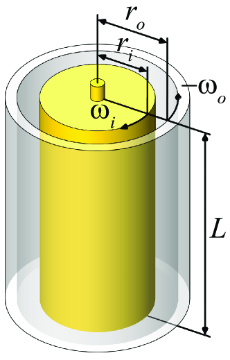
Figure 1: Schematic of the Taylor-Couette system. The system consists of two coaxial cylinders, which have an inner cylinder radius of $r_{i}$ and an outer cylinder radius of $r_{o}$. Both cylinders are of length $L$. The inner cylinder rotates with an angular velocity $\omega_{i}$ and the outer cylinder rotates with an angular velocity of $\omega_{o}$.

TC is among the most investigated systems in fluid mechanics, mainly owing to its simplicity as an experimental model for shear flows. TC is in addition a closed system, so global balances which relate the angular velocity transport to the energy dissipation can be obtained. Specifically, in Eckhardt, Grossmann & Lohse (2007) (from now on referred to as EGL 2007), an exact relationship between the global parameters and the volume averaged energy dissipation rate was derived. This relationship has an analogous form to the one which can be obtained for Rayleigh-Bénard (RB) flow, i.e. a flow in which heat is transported from a hot bottom plate to a cold top plate.

TC and RB flow have been extensively used to explore new concepts in fluid mechanics. Instabilities (Swinney & Gollub, 1981; Pfister & Rehberg, 1981; Pfister et al., 1988; Chandrasekhar, 1981; Drazin & Reid, 1981; Busse, 1967), nonlinear dynamics and chaos (Lorenz, 1963; Ahlers, 1974; Behringer, 1985; Dominguez-Lerma et al., 1986; Strogatz, 1994), pattern formation (Andereck et al., 1986; Cross & Hohenberg, 1993; Bodenschatz et al., 2000), and turbulence (Siggia, 1994; Grossmann & Lohse, 2000; Kadanoff, 2001; Lathrop et al., 1992b; Ahlers et al., 2009; Lohse & Xia, 2010) have been studied in both TC and RB and both numerically and experimentally. The main reasons behind the popularity of these systems are, in addition to the fact that they are closed systems, as mentioned previously, their simplicity due to the high amount of symmetries present. It is also worth noting that plane Couette flow is the limiting case of TC when the radius ratio $\eta=1$.

Experimental investigations of TC have a long history, dating back to the initial work in the end of the 1800s by Couette (1890) in France, who concentrated on outer cylinder rotation and developed the viscometer and Mallock (1896) in the UK, who also rotated the inner cylinder and found indications of turbulence. Later work by Wendt (1933) and Taylor (1936), greatly expanded on the system, the former measuring torques and velocities for several radius and rotation ratios in the turbulent case, and the latter being the first to mathematically describe the cells which form if the flow is linearly unstable. The subject can be traced back even further to Stokes, and even Newton. For a broader historical context, we refer the reader to Donnelly (1991).

Experimental work continued during the years (Smith & Townsend, 1982; Andereck et al., 1986; Tong et al., 1990; Lathrop et al., 1992b, a; Lewis & Swinney, 1999; van Gils et al., 2011a, b; Paoletti & Lathrop, 2011; Huisman et al., 2012b) at low and high $Ta$ numbers for different ratios of the rotation frequencies $a=-\omega_{o}/\omega_{i}$. $a$ is positive for counter–rotation and negative for co–rotation. $-a\equiv\mu$, another measure used for the ratio of rotation frequencies. This work has been complemented by numerical simulations, not only in the regime of pure inner cylinder rotation (Fasel & Booz, 1984; Coughlin & Marcus, 1996; Dong, 2007, 2008; Pirro & Quadrio, 2008), but also for eigenvalue study (Gebhardt & Grossmann, 1993), and counter-rotation at fixed $a$ (Dong, 2008). Recently (Brauckmann & Eckhardt, 2013a; Ostilla et al., 2013), simulations have also explored the effect of the outer cylinder rotation on the system at large Reynolds numbers.

The recent experiments (van Gils et al., 2011a, b; Paoletti & Lathrop, 2011; Merbold et al., 2013) and simulations (Brauckmann & Eckhardt, 2013a; Ostilla et al., 2013) have shown that at fixed $Ta$ an optimal angular momentum transport is obtained at non-zero $a_{opt}$, and that the location of this maximum $a_{opt}$ varies with $Ta$. However, both experiments and simulations have been restricted to two radius ratios, namely $\eta=0.5$ and $\eta=0.714$. The same radius ratios were also used for studies carried out on scaling laws of the torque and the “wind” of turbulence at highly turbulent Taylor numbers (Lewis & Swinney, 1999; Paoletti & Lathrop, 2011; van Gils et al., 2011b; Huisman et al., 2012b; Merbold et al., 2013). Up to now, it is not clear how the radius ratio affects the scaling laws of the system response or the recently found phenomena of optimal transport as a function of $Ta$.

Two suggestions were made to account for the radius ratio dependence of optimal transport. Van Gils et. al (2011b) wondered whether the optimal transport in general lies in or at least close to the Voronoi boundary (meaning a line of equal distance) of the Esser-Grossmann stability lines (Esser & Grossmann, 1996) in the $(Re_{o},Re_{i})$ phase space as it does for $\eta=0.714$. However, this bisector value does not give the correct optimal transport for $\eta=0.5$ (Merbold et al., 2013; Brauckmann & Eckhardt, 2013b). Therefore Brauckmann & Eckhardt (2013a) proposed a dynamic extension of the Esser-Grossmann instability theory. This model correctly gives the observed optimal transport (within experimental error bars) between $\eta=0.5$ and $\eta=0.714$ for three experimental data sets (Wendt, 1933; Paoletti & Lathrop, 2011; van Gils et al., 2011b) and one numerical data set (Brauckmann & Eckhardt, 2013b), but it is not clear how it performs outside the $\eta$-range $[0.5,0.714]$.

In this paper, we study the following questions: how does the radius ratio $\eta$ affect the flow? How are the scaling laws of the angular momentum transport affected? What is the role of the geometric parameter called pseudo-Prandtl number $\sigma$ introduced in EGL2007? Can the effect of the radius ratio be interpreted as a kind of non-Oberbeck-Boussinesq effect, analogous to this effect in Rayleigh-Bénard flow? Finally, are the predictions and insights of van Gils et al. (2011b), Ostilla et al. (2013) and Brauckmann & Eckhardt (2013b) on the optimal transport also valid for other values of $\eta$?

In order to answer these questions, both direct numerical simulations (DNS) and experiments have been undertaken. Numerical simulations, with periodic axial boundary conditions, have been performed using the finite–difference code previously used in Ostilla et al. (2013). In these simulations, three more values of $\eta$ have been investigated: one in which the gap is larger ($\eta=0.5$), and two in which the gap is smaller ($\eta=0.833$ and $0.909$). With the previous simulations from Ostilla et al. (2013) at $\eta=0.714$, a total of four radius ratios has been analyzed.

In both experiments and numerics, only one aspect ratio $\Gamma$ has been studied for every radius ratio. Since the work of Benjamin (1978) it is known that multiple flow states with a different amount of vortex pairs can coexist in TC for the same non-dimensional flow parameters. However, with increased driving, the bifurcations become less important and many branches do not survive. Indeed, Lewis & Swinney (1999) found that for pure inner cylinder rotation only one branch with 8 vortices (for $\Gamma=11.4$ and $\eta=0.714$) remains when $Re_{i}$ is increased above $2\cdot 10^{4}$. As the Reynolds numbers reached in the experiments greatly exceed this value we do not expect to see the effect of multiple states in the current experimental results.

For the numerical simulations, axially periodic boundary conditions have been taken. Brauckmann & Eckhardt (2013a) already studied the effect of the axial periodicity length on the system, and found that for a fixed vortical wavelength, the number of vortices does not affect the overall flow behaviour. It was also found that, in analogy to experiments, the effect of vortical wavelength, and hence of multiple states, becomes smaller with increased driving.

Figure 2 shows the ($Ta$,$1/Ro$) parameter space explored in the simulations for the four selected values of the radius ratio $\eta$. A higher density of points has been used in places where the global response ($Nu_{\omega}$, $Re_{w}$) of the flow shows more variation with the control parameters $Ta$ and $1/Ro$. A fixed aspect ratio of $\Gamma=2\pi$ has been taken for all simulations, and axially periodic boundary conditions have been used. These simulations have the same upper bounds of $Ta$ (or $Re_{i}$) as the ones of Ostilla et al. (2013).

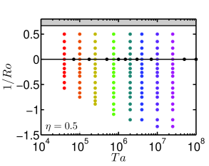
(a)

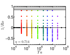
(b)

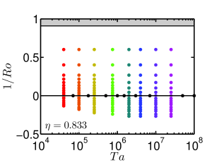
(c)

(d)

Figure 2: Control parameter phase space which was numerically explored in this paper in the ($Ta$, $1/Ro$) representation. From top-left to bottom-right: $\eta=0.5$, $0.714$, $0.833$ and $0.909$. $\Gamma=2\pi$ was fixed, and axial periodicity was employed. The grey-shaded area signals boundary conditions for which the angular momentum $L=r^{2}\omega$ of the outer cylinder ($L_{o}$) is larger than the angular momentum of the inner cylinder ($L_{i}$). This causes the flow to have an overall transport of angular momentum towards the inner cylinder. In this region, the Rayleigh stability criterium applies, which states that if $dL^{2}/dr>0$ the flow is linearly stable to axisymmetric perturbations.

In addition to these simulations, experiments have been performed with the Twente Turbulent Taylor-Couette ($T^{3}C$) facility, with which we achieve larger Ta numbers. Details of the setup are given in van Gils et al. (2011a). Once again, four values of $\eta$ have been investigated, but, due to experimental constraints, we have been limited to investigate only smaller gap widths, i.e. values $\eta\geq 0.714$, namely $\eta=0.714$, $0.769$, $0.833$ and $0.909$. The experimentally explored parameter space are shown in Fig. 3.

(a)

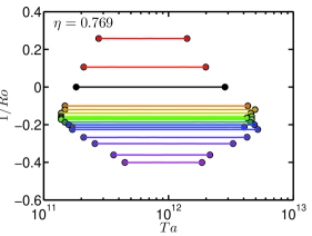
(b)

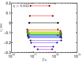
(c)

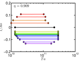
(d)

Figure 3: Control parameter phase space which was explored in experiments in the ($Ta$, $Ro^{-1}$) representation for $\eta=0.716$ (top-left), $\eta=0.769$ (top-right), $\eta=0.833$ (bottom-left) and $\eta=0.909$ (bottom-right).

The structure of the paper is as follows. In sections 2 and 3, we start by describing the numerical code and the experimental setup, respectively. In section 4, the global response of the system, quantified by the non-dimensionalized angular velocity current $Nu_{\omega}$ is analyzed. To understand the global response, we analyze the local data which can be obtained from the DNS simulations in section 5. Angular velocity profiles in the bulk and in the boundary layers are analyzed and related to the global angular velocity optimal transport. We finish in section 6 with a discussion of the results and an outlook for further investigations.

2 Numerical method

In this section, the used numerical method is explained in some detail. The rotating frame in which the Navier-Stokes equations are solved and the employed non-dimensionalizations are introduced in the first section. This is followed by detailing the spatial resolution checks which have been performed.

2.1 Code description

The employed code is a finite difference code, which solves the Navier-Stokes equations in cylindrical coordinates. A second–order spatial discretization is used, and the equations are advanced in time by a fractional time integration method. This code is based on the so-called Verzicco-code, whose numerical algorithms are detailed in Verzicco & Orlandi (1996). A combination of MPI and OpenMP directives are used to achieve large scale parallelization. This code has been extensively used for Rayleigh-Bénard flow; for recent simulations see Stevens et al. (2010, 2011). In the context of TC flow, Ostilla et al. (2013) already validated the code for $\eta=0.714$.

The flow was simulated in a rotating frame, which was chosen to rotate with $\Omega=\omega_{o}\boldsymbol{e}_{z}$. This was done in order to simplify the boundary conditions. In that frame the outer cylinder is stationary for any value of $a$, while the inner cylinder has an azimuthal velocity of $u_{\theta}(r=r_{i})=r_{i}(\omega^{\ell}_{i}-\omega^{\ell}_{o})$, where the $\ell$ superscript denotes variables in the lab frame, while no superscript denotes variables in the rotating frame. We then choose the inner cylinder rotation rate in the rotating frame as the characteristic velocity of the system $U\equiv|u_{\theta}(r_{i})|=r_{i}|\omega_{i}-\omega_{o}|$ and the characteristic length scale $d$ to non-dimensionalize the equations and boundary conditions.

Using this non-dimensionalization, the inner cylinder velocity boundary condition simplifies to: $\hat{u}_{\theta}(r=r_{i})=\text{sgn}(\omega_{i}-\omega_{o})$. In this paper, $\omega_{i}-\omega_{o}$ is always positive. Thus, in this rotating frame the flow geometry is simplified to a pure inner cylinder rotation with the boundary condition $\hat{u}_{\theta}(r_{i})=1$. The outer cylinder’s effect on the flow is felt as a Coriolis force in this rotating frame of reference. The Navier-Stokes equations then read:

$$\frac{\partial\hat{\boldsymbol{u}}}{\partial\hat{t}}+\hat{\boldsymbol{u}}\cdot\hat{\nabla}\hat{\boldsymbol{u}}=-\hat{\nabla}\hat{p}+\left(\displaystyle\frac{f(\eta)}{Ta}\right)^{1/2}\hat{\nabla}^{2}\hat{\boldsymbol{u}}+Ro^{-1}{\boldsymbol{e}_{z}}\times\hat{\boldsymbol{u}}~{},$$ (3)

where $Ro$ was defined previously in Eq. 2, and $f(\eta)$ is

$$f(\eta)=\displaystyle\frac{(1+\eta)^{3}}{8\eta^{2}}~{}.$$ (4)

It is useful to continue the non-dimensionalization by defining the normalized radius $\tilde{r}=(r-r_{i})/d$ and the normalized height $\tilde{z}=z/d$. We define the time- and azimuthally-averaged velocity field as:

$$\hat{\mathrm{bar}{\boldsymbol{u}}}(r,z)=\langle\hat{\boldsymbol{u}}(\theta,r,z,t)\rangle_{\theta,t}~{},$$ (5)

where $\langle\phi(x_{1},x_{2},...,x_{n})\rangle_{x_{i}}$ indicates averaging of the field $\phi$ with respect to $x_{i}$.

To quantify the torque in the system, we first note that the angular velocity current

$$J^{\omega}=r^{3}(\langle u_{r}^{\ell}\omega^{\ell}\rangle_{\theta,z,t}-\nu\partial_{r}\langle\omega^{\ell}\rangle_{\theta,z,t})$$ (6)

is conserved, i.e. independent on the radius $r$ (EGL 2007). $J^{\omega}$ represents the current of angular velocity from the inner cylinder to the outer cylinder (or vice versa). The first term is the convective contribution to the transport, while the second term is the diffusive contribution.

In the state with the lowest driving, and ignoring end plate effects, a laminar, time independent velocity field which is purely azimuthal, $u^{\ell}_{\theta}(r)=Ar+B/r$, with $u_{r}=u_{z}=0$, is induced by the rotating cylinders. This laminar flow produces an angular velocity current $J_{0}^{\omega}$, which can be used to nondimensionalize the angular velocity current and a non-zero dissipation rate $\epsilon_{u,0}$.

$$Nu_{\omega}=\displaystyle\frac{J^{\omega}}{J_{0}^{\omega}}.$$ (7)

$Nu_{\omega}$ can be seen as an angular velocity “Nusselt” number.

When $J^{\omega}$, and therefore $Nu_{\omega}$ are calculated numerically, the values will depend on the radial position, due to finite time averaging. We can define $\Delta_{J}$ to quantify this radial dependence as:

$$\Delta_{J}=\displaystyle\frac{\max(J^{\omega}(r))-\min(J^{\omega}(r))}{\langle J^{\omega}(r)\rangle_{r}}=\displaystyle\frac{\max(Nu_{\omega}(r))-\min(Nu_{\omega}(r))}{\langle Nu_{\omega}(r)\rangle_{r}}$$ (8)

which analytically equals zero but will deviate when calculated numerically.

The convective dissipation per unit mass can be calculated either from its definition as a volume average of the local dissipation rate for an incompressible fluid,

$$\varepsilon_{u}=\epsilon^{\ell}_{u}=\displaystyle\frac{\nu}{2}\left\langle(\partial_{i}^{\ell}u_{j}+\partial_{j}^{\ell}u_{i})^{2}\right\rangle_{V,t},$$ (9)

or a global balance can also be used. The exact relationship (EGL 2007)

$$\epsilon^{\ell}_{u}-\epsilon^{\ell}_{u,0}=\displaystyle\frac{\nu^{3}}{d^{4}}\sigma^{-2}Ta(Nu_{\omega}-1)~{},$$ (10)

where $\epsilon_{u,0}$ is the volume averaged dissipation rate in the purely azimuthal laminar flow, links the volume averaged dissipation to the global driving $Ta$ and response $Nu_{\omega}$.

This link can be and has been used for code validation and for checking spatial resolution adequateness. The volume averaged dissipation can be calculated from both (9) and (10) and later checked for sufficient agreement. We define the quantity $\Delta_{\epsilon}$ as the relative difference between the two ways of numerically calculating the dissipation, namely either via $Nu_{\omega}$ with eq. 10 or directly from the velocity gradients, eq. 9:

$$\Delta_{\epsilon}=\displaystyle\frac{\nu^{3}d^{-4}\sigma^{-2}Ta(Nu_{\omega}-1)+\epsilon_{u,0}-\frac{\nu}{2}\left\langle(\partial_{i}u^{\ell}_{j}+\partial^{\ell}_{j}u_{i})^{2}\right\rangle_{V,t}}{\frac{\nu}{2}\left\langle(\partial^{\ell}_{i}u_{j}+\partial^{\ell}_{j}u_{i})^{2}\right\rangle_{V,t}}~{}.$$ (11)

$\Delta_{\epsilon}$ is equal to $0$ analytically, but will deviate when calculated numerically. The deviation of $\Delta_{J}$ and $\Delta_{\epsilon}$ from zero is an indication of the adequateness of the resolution.

We would like to emphasize that the requirement for $\Delta_{J}<0.01$ is much stricter than torque balance, which can simply be expressed as $Nu_{\omega}(r_{i})=Nu_{\omega}(r_{o})$. As analyzed in Ostilla et al. (2013), a value of less than $1\%$ for $\Delta_{J}$ and about $1\%$ for $\Delta_{\epsilon}$ is linked to grid adequateness at the Taylor number simulated. To ensure convergence in time, the time-averages of the Nusselt number and the energy dissipation calculated locally (equation 9) were also checked to converge in time within $1\%$.

2.2 Resolution checks

Spatial resolution checks were performed in two ways. First, as mentioned previously, the values of $\Delta_{J}$ and $\Delta_{\epsilon}$ were checked. As an additional check, simulations at selected values of $Ta$ were performed at a higher resolution. As the explored parameter space is large, these checks were performed only for the highest value of $Ta$ simulated for the grid size. A lower driving of the flow for the same grid size is expected to have a smaller error due to spatial discretization, as spatial discretization errors increase with increased $Re$, and thus increased $Ta$.

Concerning the temporal resolution there are numerical and physical constraints; the former requires a time step small enough to keep the integration scheme stable and this is achieved by using an adaptive time step based on a Courant–Frederich–Lewy ($CFL$) criterium. The $3^{\rm rd}$–order Runge–Kutta time–marching algorithm allows for a $CFL$ of up to $\sqrt{3}$, but this can be reduced due to the implicit factorization of the viscous terms. For safety, the maximum $CFL$ has been taken as $1.4$. From the physical point of view, the time step size must also be small enough to properly describe the fast dynamics of the smallest flow scale which is the Kolmogorov scale. Although the time step size should be determined by the most restrictive among the two criteria above, our experience suggests that as long as the $CFL$ number criterion is satisfied, which guarantees numerical stability, the results become insensitive to the time step size and all the flow scales are adequately described temporally. Direct confirmation of this statement can be found in Ostilla et al. (2013).

The results for $\eta=0.5$, $0.833$, and $0.909$ are presented in Table 1. Uniform discretization was used in azimuthal and axial directions. In the radial direction, points were clustered near the walls by using hyperbolic tangent-type clustering, or a clipped Chebychev type clustering for higher values of $Ta$. A table including the results for the spatial resolution tests at $\eta=0.714$ can be found in Ostilla et al. (2013).

$\eta$	$Ta$	$N_{\theta}$ x $N_{r}$ x $N_{z}$	$Nu_{\omega}$	100$\Delta_{J}$	100$\Delta_{\epsilon}$	Case
$0.5$	$2.5\cdot 10^{5}$	100x100x100	2.03372	0.30	1.11	R
$0.5$	$2.5\cdot 10^{5}$	150x150x150	2.03648	0.76	0.89	E
$0.5$	$7.5\cdot 10^{5}$	150x150x150	2.56183	0.47	0.92	R
$0.5$	$7.5\cdot 10^{5}$	256x256x256	2.55673	0.74	0.31	E
$0.5$	$1\cdot 10^{7}$	300x300x300	4.23128	0.33	1.07	R
$0.5$	$1\cdot 10^{7}$	400x400x400	4.22574	0.97	1.06	E
$0.5$	$2.5\cdot 10^{7}$	350x350x350	5.07899	0.85	1.12	R
$0.5$	$2.5\cdot 10^{7}$	512x512x512	5.08193	0.87	1.98	E
$0.5$	$5\cdot 10^{7}$	768x512x1536	6.08284	0.45	1.56	R
$0.5$	$1\cdot 10^{8}$	768x512x1536	7.48561	1.46	0.88	R
$0.833$	$2.5\cdot 10^{5}$	180x120x120	2.72293	0.21	0.76	R
$0.833$	$2.5\cdot 10^{5}$	300x180x180	2.72452	0.29	0.29	E
$0.833$	$1\cdot 10^{7}$	384x264x264	7.07487	0.29	0.61	R
$0.833$	$1\cdot 10^{7}$	512x384x384	7.17245	0.13	1.16	E
$0.833$	$2.5\cdot 10^{7}$	512x384x384	8.62497	0.71	1.05	R
$0.833$	$2.5\cdot 10^{7}$	768x576x576	8.51678	0.90	1.26	E
$0.833$	$5\cdot 10^{7}$	512x384x384	9.68437	0.26	2.92	R
$0.833$	$1\cdot 10^{8}$	768x576x576	11.4536	0.89	2.29	R
$0.909$	$2.5\cdot 10^{5}$	180x120x120	2.31902	0.16	0.91	R
$0.909$	$2.5\cdot 10^{5}$	300x200x200	2.30810	0.07	0.17	E
$0.909$	$2\cdot 10^{6}$	256x180x180	3.76826	0.55	0.49	R
$0.909$	$2\cdot 10^{6}$	384x256x256	3.77532	0.39	0.21	E
$0.909$	$2.5\cdot 10^{7}$	384x256x256	7.83190	0.43	3.15	R
$0.909$	$2.5\cdot 10^{7}$	450x320x320	7.86819	0.81	2.07	E
$0.909$	$5\cdot 10^{7}$	2305x400x1536	9.74268	0.46	1.02	R
$0.909$	$1\cdot 10^{8}$	2305x400x1536	11.3373	0.57	1.06	R

Table 1: Resolution tests for $\Gamma=2\pi$ and $\eta=0.5$, $0.833$ and $0.909$. The first column displays the radius ratio, the second column displays the Taylor number, the third column displays the resolution employed, the fourth column the calculated $Nu_{\omega}$, the fifth column and sixth colums the relative discrepancies $\Delta_{J}$ and $\Delta_{\epsilon}$, and the last column the ’case’: (R)esolved and (E)rror reference. $\Delta_{\epsilon}$ is positive, and exceeds the $1\%$ threshold reported in Ostilla et al. (2013) for some cases at the largest $\eta$, but even so resolution appears to be sufficient as variations of $Nu_{\omega}$ are small.

3 Experimental setup

The Twente Turbulent Taylor-Couette ($\text{T}^{3}\text{C}$) apparatus has been built to obtain high $Ta$ numbers. It has been described in detail in van Gils et al. (2011a) and van Gils et al. (2012). The inner cylinder with outside radius $r_{i}=$0.200\text{\,}\mathrm{m}$$ consists of three sections. The total height of those axially stacked sections is $L=$0.927\text{\,}\mathrm{m}$$. We measure the torque only on the middle section of the inner cylinder, which has a height of $L_{\text{mid}}=$0.536\text{\,}\mathrm{m}$$, to reduce the effect of the torque losses at the end-plates in our measurements. This approach has already been validated in van Gils et al. (2012). The transparent outer cylinder is made of acrylic and has an inside radius of $r_{o}=$0.279\text{\,}\mathrm{m}$$. We vary the radius ratio by reducing the diameter of the outer cylinder by adding a ‘filler’ that is fixed to the outer cylinder and sits between the inner and the outer cylinder, effectively reducing $r_{o}$ while keeping $r_{i}$ fixed. We have 3 fillers giving us 4 possible outer radii: $r_{o}=$0.279\text{\,}\mathrm{m}$$ (without any filler), $0.26\text{\,}\mathrm{m}$, $0.24\text{\,}\mathrm{m}$, and $0.22\text{\,}\mathrm{m}$, giving experimental access to $\eta=0.716$, $0.769$, $0.833$, and $0.909$, respectively. Note that by reducing the outer radius, we not only change $\eta$, but also change $\Gamma=L/(r_{o}-r_{i})$ from $\Gamma(\eta=0.716)=11.68$ to $\Gamma(\eta=0.909)=46.35$.

For high $Ta$ the heating up of the system becomes apparent and it has to be actively cooled in order to keep the temperature constant. We cool the working fluid (water) from the top and bottom end plates and maintain a constant temperature within $\pm 0.5K$ throught both the spatial extent and the time run of the experiment. The setup has been constructed in such a way that we can rotate both cylinders independently while keeping the setup cooled.

As said before, we measure the torque on the middle inner cylinder. We do this by measuring the torque that is transferred from the axis to the cylinder by using a load-cell that is inside the aforementioned cylinder. Torque measurements are performed using a fixed procedure: the inner cylinder is spun up to its maximum rotational frequency of $20\text{\,}\mathrm{Hz}$ and kept there for several minutes. Then the system is brought to rest. The cylinders are then brought to their initial rotational velocities (with the chosen $1/Ro$), corresponding to a velocity for which the torque is accurate enough; generally of order 2–$3\text{\,}\mathrm{Hz}$. We then slowly increase both velocities over 3-6 hours to their final velocities while maintaining $1/Ro$ fixed during the entire experiment. During this velocity ramp we continuously acquire the torque of this quasi-stationary state. The calibration of the system is done in a similar way; first we apply the maximum load on the system, going back to zero load, and then gradually adding weight while recording the torque. These procedures ensure that hysteresis effects are kept to a minimum, and that the system is always brought to the same state before measuring. More details about the setup can be found in van Gils et al. (2011a).

Local velocity measurements are done by laser Doppler anemometry (LDA). We measure the azimuthal velocity component by focusing two beams in the radial-azimuthal plane. We correct for curvature effects of the outer cylinder by using a ray-tracer, see Huisman et al. (2012a). The velocities are measured at midheight ($z=L/2$) unless specified otherwise. For every measurement position we measured long enough such as to have a statistically stationary result, for which about $10^{5}$ samples were required for every data point. This ensured a statistical convergence of $<1\%$.

4 Global response: Torque

In this section, the global response of the TC system for the four simulated radius ratios is presented. This is done by measuring the scaling law(s) of the non-dimensional torque $Nu_{\omega}$ as function(s) of $Ta$. The transition between different types of local scaling laws in different $Ta$-ranges is investigated, and related to previous simulations (Ostilla et al., 2013) and experiments (van Gils et al., 2012).

4.1 Pure inner cylinder rotation

The global response of the system is quantified by $Nu_{\omega}$. By definition, for purely azimuthal laminar flow, $Nu_{\omega}=1$. Once the flow is driven stronger than a certain critical $Ta$, large azimuthal roll structures appear, which enhance angular transport through a large scale wind.

Figure 4 shows the response of the system for increasing $Ta$ in case of pure inner cylinder rotation for four values of $\eta$. Experimental and numerical results are shown in the same panels, covering different ranges and thus complementary, but consistent with each other. Numerical results for $\eta=0.714$ from Ostilla Monico et al. (2013) have been added to both panels.

(a)

(b)

Figure 4: The global system response for pure inner cylinder rotation as function of the driving $Ta$: The top panel shows $Nu_{\omega}-1$ vs $Ta$ for both simulations (points on the left of the graph) and experiments (lines on the right of the graph). Numerical data from Ostilla Monico et al. (2013) for $\eta=0.714$ have been added to these figures. The bottom panel shows the compensated Nusselt ($(Nu_{\omega}-1)/Ta^{1/3}$) versus $Ta$, with added lines with scaling law $Ta^{0.20}$ and $Ta^{0.39}$ to guide the eye.

As has already been noticed in Ostilla et al. (2013) for $\eta=0.714$, a change in the local scaling law relating $Ta$ to $Nu_{\omega}$ occurs at around $Ta\approx 3\cdot 10^{6}$. We can interpret these changes in the same way as Ostilla et al. (2013) and relate the transition in the $Ta$-$Nu_{\omega}$ local scaling law to the break up of coherent structures.

It is also worth mentioning that the exponent in the local scaling laws in the regime before the transition depends on the radius ratio. This can be seen in the compensated plot, and explains the curve crossings that we see in the graphs.

For experiments (solid lines of figure 4), a different local scaling law can be seen. In this case the experiments are performed at much higher $Ta$ than the simulations. The scaling $Nu_{\omega}\sim Ta^{0.38}$ can be related to the so called “ultimate” regime, a regime where the boundary layers have become completely turbulent (Grossmann & Lohse, 2011, 2012; Huisman et al., 2013). As indicated for the case at $\eta=0.714$ we expect that for increasing $Ta$ also the simulations become turbulent enough to reach this scaling law (cf. Ostilla Monico et al. (2013)). In this regime, the local scaling law relating $Ta$ and $Nu_{\omega}$ has no dependence on $\eta$ and thus is universal.

In both experiment and simulation with the largest $Ta$, the value of $\eta$ corresponding to the smallest gap, i.e. $\eta=0.909$, has the highest angular velocity transport ($Nu_{\omega}$) at a given $Ta$. This can be phrased in terms of the pseudo-Prandtl-number $\sigma$, introduced in EGL2007. As a smaller gap means a smaller $\sigma$, we thus find a decrease of $Nu_{\omega}$ with increasing $\sigma$, for the drivings explored in experiments, similarly as predicted Grossmann & Lohse (2001) and found Xia et al. (2002) for $Nu(Pr)$ in RB convection for $Pr>1$.

4.2 Rossby number dependence

In this subsection, the effect of outer cylinder rotation on angular velocity transport will be studied. Previous experimental and numerical work at $\eta=0.714$ (Paoletti & Lathrop, 2011; van Gils et al., 2011b; Ostilla et al., 2013; Brauckmann & Eckhardt, 2013a) revealed the existence of an optimum transport where, for a given $Ta$, the transport of momentum is highest at a Rossby number $Ro^{-1}_{opt}$, which depends on $Ta$ and saturates around $Ta\sim 10^{10}$. In this subsection, this work will be extended to the other values of $\eta$.

Figure 5 shows the results of the numerical exploration of the $Ro^{-1}$ parameter space between $Ta=4\cdot 10^{4}$ and $Ta=2.5\cdot 10^{7}$. The shape of $Nu_{\omega}=Nu_{\omega}(Ro^{-1})$ curves and the position of $Ro^{-1}_{opt}$ depends very strongly on $\eta$ in the $Ta$ range studied in numerics. For the largest gap (i.e., $\eta=0.5$), the optimum can be seen to be in the counter–rotating range (i.e., $Ro^{-1}<0$) as long as $Ta$ is high enough. On the other hand, for the smallest gap (i.e., $\eta=0.909$), the optimum is at co–rotation (i.e., $Ro^{-1}>0$) in the whole region studied. The other values of studied $\eta$ reveal an intermediate behavior. Optimum transport is located for co–rotation at lower values of $Ta$ and slowly moves towards counter–rotation. For all values of $\eta$, when the driving is increased, $Ro^{-1}_{opt}$ tends to shift to more negative values.

For two values of $Ta$ ($Ta=4\cdot 10^{6}$ and $Ta=10^{7}$) for a radius ratio $\eta=0.5$, two distinct peaks can be seen in the $Nu_{\omega}(Ro^{-1})$ curve. This can be understood by looking at the flow topology. For $Ro^{-1}=0$, three distinct rolls can be seen. However, when decreasing $Ro^{-1}$, the rolls begin to break up. Some remnants of large-scale structures can be seen, but these are weaker than the $Ro^{-1}=0$ case. Having a large-scale roll helps the transport of angular momentum, leading to the peak in $Nu_{\omega}$ at $Ro^{-1}=0$. Further increasing the driving causes the rolls to also break up for $Ro^{-1}=0$, and eliminates the anomalous peak.

(a)

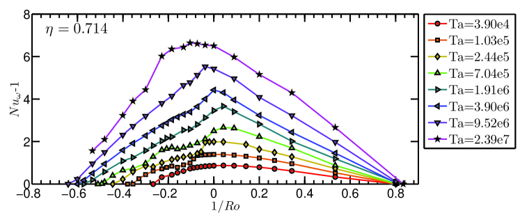
(b)

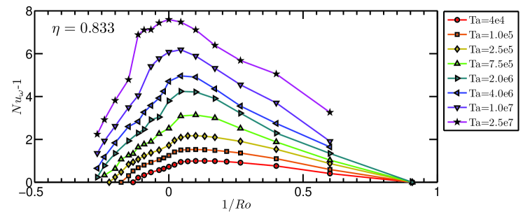
(c)

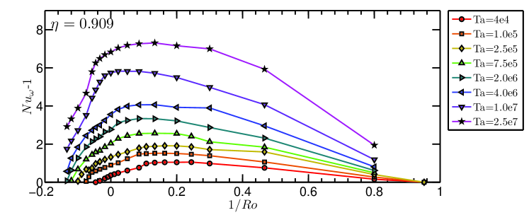
(d)

Figure 5: $Nu_{\omega}-1$ versus $Ro^{-1}$ for the four values of $\eta$ studied numerically, $\eta=0.5$ (top), $0.714$, $0.833$ and $0.909$ (bottom). The shape of the curve and the position of the maximum depend very strongly on both $Ta$ and $\eta$.

The shift seen in the numerics may or may not continue with increasing $Ta$. The experiments conducted explore a parameter space of $10^{10}<Ta<10^{13}$ and thus serve to explore the shift at higher driving. Figure 6 presents the obtained results. The left panel shows $Nu_{\omega}$ versus $Ta$ for all measurements. The right panel shows the exponent $\gamma$, obtained by fitting a least-square linear fit in the log–log plots. Across the $\eta$ and $Ro^{-1}$ range studied, the average exponent is $\gamma\approx 0.39$. This value is used in figure 7b to compensate $Nu_{\omega}$. The horizontality of all data points reflects the good scaling and the universality of this ultimate scaling behaviour $Nu_{\omega}\propto Ta^{0.39}$.

(a)

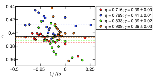
(b)

Figure 6: The left panel shows $Nu_{\omega}$ versus $Ta$ for all values of $\eta$ and $Ro^{-1}$ studied in experiments. The right panel shows the exponent $\gamma$ of the scaling law $Nu_{\omega}\propto Ta^{\gamma}$ for various $Ro^{-1}$, obtained by a least-square linear fit in log-log space. The average value of $\gamma$ for each $\eta$ is represented by the dashed lines, while the solid line represents the average value of $\gamma=0.39$ for all $\eta$, which will be used for compensating $Nu_{\omega}$.

To determine the optimal rotation ratio for the experimental data, a $Ta$-averaged compensated Nusselt $\langle Nu_{\omega}/Ta^{0.39}\rangle_{Ta}$ was used. This is defined as:

$$\langle Nu_{\omega}/Ta^{0.39}\rangle_{Ta}=\displaystyle\frac{1}{Ta_{max}-Ta_{co}}\int^{Ta_{max}}_{Ta_{co}}Nu_{\omega}/Ta^{0.39}dTa,$$ (12)

where $Ta_{max}$ is the maximum value of $Ta$ for every ($\eta,Ro^{-1}$) dataset, and $Ta_{co}$ is a cut-off $Ta$ number used for the larger $\eta$ ($Ta_{co}=2\cdot 10^{11}$ for $\eta=0.833$ and $Ta_{co}=3\cdot 10^{10}$ for $\eta=0.909$) to exclude the initial part of the $Nu_{\omega}/Ta^{0.39}$ data points which seem to have a different scaling for some of the values of $Ro^{-1}$ explored. For the smaller values of $\eta$, $Ta_{co}=Ta_{min}$, the minimum value of $Ta$ for every ($\eta,Ro^{-1}$) dataset. An error bar on this average is estimated as one standard deviation of the data from the computed average.

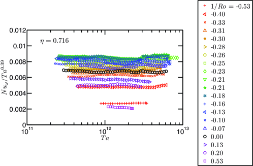
(a)

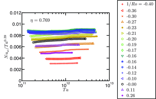
(b)

Figure 7: The four panels show $Nu_{\omega}/Ta^{0.39}$ vs. $Ta$ for all explored values of $Ro^{-1}$ for the four studied values of $\eta$: $\eta=0.714$ (top-left), $0.769$ (top-right), $0.833$ (bottom-left), and $0.909$ (bottom-right). The scaling law $Nu_{\omega}\sim Ta^{0.39}$ is seen to approximately hold throughout the whole parameter space explored. No trends can be appreciated which would lead us to expect further shift of the optimum with increased driving. Dashed lines, indicating the cut-off regions used for determining $\langle Nu_{\omega}/Ta^{0.39}\rangle_{Ta}$ have been plotted for $\eta=0.833$ and $\eta=0.909$.

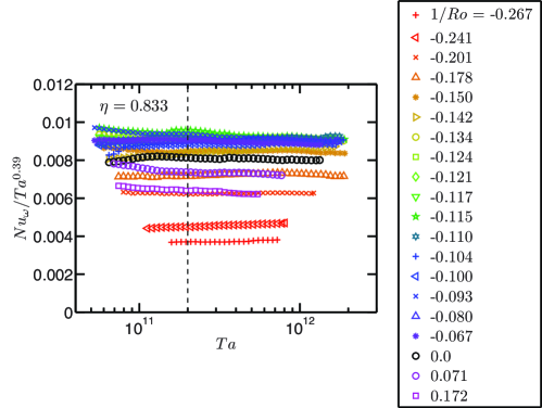
(c)

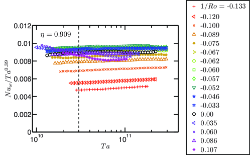
(d)

The two panels of figure 8 show $\langle Nu_{\omega}/Ta^{0.39}\rangle_{Ta}$ as a function of $Ro^{-1}$ or alternatively of $a$ for the four values of $\eta$ considered in experiments. The increased driving changes the characteristics of the flow. This is reflected in the very different shapes of the $Ro^{-1}$-dependence of $Nu_{\omega}$ when comparing figures 5 and 8, and in the shift of $Ro^{-1}_{opt}$.

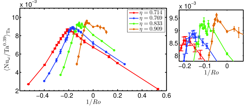
(a)

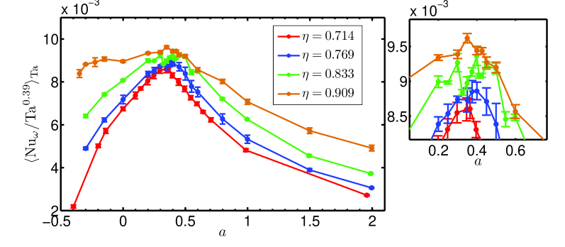
(b)

Figure 8: The panels show $\langle Nu_{\omega}/Ta^{0.39}\rangle_{Ta}$ versus either $Ro^{-1}$ (top) or $a$ (bottom) at the cut-off region highlighted in figure 7b for the values of $\eta$ studied experimentally. Insets containing a zoom-in around the optimum have been added for clarity. Error bars indicate one standard deviation from the mean value, and are too small to be seen for most data points. There is a strong $\eta$-dependence of the curve $Nu_{\omega}/Ta^{0.39}$ versus $Ro^{-1}$, even at the largest drivings studied in experiments. Optimal transport is located at $Ro^{-1}_{opt}=-0.20$ for $\eta=0.714$, $Ro^{-1}_{opt}=-0.15$ for $\eta=0.769$, $Ro^{-1}_{opt}=-0.10$ for $\eta=0.833$ and $Ro^{-1}_{opt}=-0.05$ for $\eta=0.909$, corresponding to $a\approx 0.33-0.35$ for all values of $\eta$. In the bottom panel, the maximum of the graph is less pronounced, i.e. it becomes more flat with increasing $\eta$. In the limit $\eta\to 1$, $a$ does not tend to a finite limit, while $Ro^{-1}$ does. This result highlights the advantage of using $Ro^{-1}$ instead of $a$ as a control parameter.

To summarize these effects, figure 9 presents both the $95\%$ peak width $\Delta Ro^{-1}_{max}$ and the position of optimal transport $Ro^{-1}_{opt}$ determined as the realization with the maximum torque as a function of $Ta$ and $\eta$ obtained from numerics as well as the asymptotic value from experiments. The peak width $\Delta Ro^{-1}_{max}$ is defined as:

$$\Delta Ro^{-1}_{max}=\displaystyle\frac{\displaystyle\int_{Ro^{-1}_{-0.95}}^{Ro^{-1}_{0.95}}Nu_{\omega}(Ro^{-1})dRo^{-1}}{\mathrm{max}(Nu_{\omega}-1)}$$ (13)

where $Ro^{-1}_{-0.95}$ and $Ro^{-1}_{0.95}$ are the values of $Ro^{-1}$ for which $Nu_{\omega}$ is $95\%$ of the peak value.

The $95\%$ peak width can be seen to vary with driving, reflecting what is seen in figure 5. The shape of the $Ro^{-1}$-$Nu_{\omega}$ curve is highly dependent of both $\eta$ and $Ta$. $Ro^{-1}_{opt}$ shows a very large variation across the $Ta$ range studied in numerics. The shift of the $Ro^{-1}_{opt}$ with $Ta$ is expected to continue until it reaches the value found in the experiments. This can be seen in the right panel of figure 5 for $\eta=0.5$ to $\eta=0.833$. For $\eta=0.909$ , the trend seems to change for the last point. However, this is due to the very large and flat peak of the $Nu_{\omega}(Ro^{-1})$ curve- this can also be seen in the left panel and in figure 5d.

One may also ask the question: has the value of $Ro^{-1}_{opt}$ already saturated in our experiments? Figure 7b shows the trend for $Nu_{\omega}$ for increasing $Ta$. This trend does not seem to vary much for different values of $Ro^{-1}$. Therefore, we expect the value of $Ro^{-1}_{opt}$ to have already reached saturation in our experiments.

We can compare these new experimental results to the available results from the literature, the speculation made in van Gils et al. (2012) and the prediction made in Brauckmann & Eckhardt (2013b) for the dependence of the saturated $a_{opt}$ on $\eta$. This is shown in figure 10. Both dependencies are shown to deviate substantially from the experimental results obtained in the present work. Even if the speculation from van Gils et al. (2012) appears to be better for this $\eta$-range, for previous experimental data at $\eta=0.5$, it is in clear difference with the experimentally measured value for optimal transport by Merbold et al. (2013).

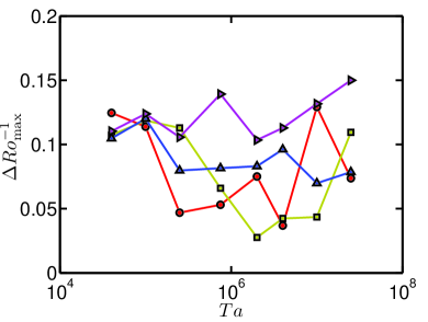
(a)

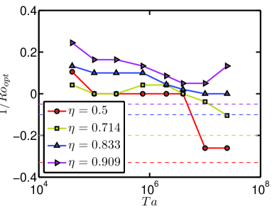
(b)

Figure 9: In the left panel, $95\%$ peak width $\Delta Ro^{-1}_{max}$ vs $Ta$ for the four values of $\eta$ analyzed in numerics. The peak width can be seen to vary with driving, and for smaller gaps is larger for larger values of $Ta$. In the right panel, $Ro^{-1}_{opt}$ vs $Ta$ for the same four values of $\eta$. The location of the optimal transport has a very strong dependence on the driving, especially for the largest values of $\eta$. As driving increases beyond the numerically studied range and overlaps with experiments, $Ro^{-1}_{opt}$ should tend to the experimentally found values, represented as dashed lines in the figure. The asymptote for $\eta=0.5$ is obtained from Merbold et al. (2013). The trend appears to be less clear for $\eta=0.909$, but this might be understandable from the peak width at the highest driving $Ta$.

Figure 10: State-of-the-art data for $a_{opt}(\eta)$, from both experiments (Wendt, 1933; Paoletti & Lathrop, 2011; Merbold et al., 2013) and numerics (Brauckmann & Eckhardt, 2013b). The speculation of van Gils et al. (2012) and the prediction of Brauckmann & Eckhardt (2013b) are plotted as lines on the graph. The new experimental results deviate up substantially from both predictions, even when taking into account error bars.

This section has shown that the radius ratio has a very strong effect on the global response and especially on optimal transport. Significantly increased transport for co–rotation has been found at the lowest drivings based on the DNS results. This finding was already reported in Ostilla et al. (2013) for $\eta=0.714$, but the transport increase was marginal. For $\eta=0.833$ and especially for $\eta=0.909$ the transport can be increased up to three times. The shift of $Ro^{-1}_{opt}$ has also been seen to be much bigger and to happen in a much slower way for smaller gaps. The reason for this will be studied in Section 5, using the local data obtained from experiments and numerics.

5 Local results

In this section, the local angular velocity profiles will be analyzed. Angular velocity is the transported quantity in TC flow and shows the interplay between the bulk, where the transport is convection dominated, and the boundary-layers, where the transport is diffusion dominated. Numerical profiles and experimental profiles obtained from LDA will be shown. The angular velocity gradient in the bulk will be analyzed and connected to the optimal transport. In addition, the boundary layers will be analyzed and compared to the results from the analytical formula from EGL 2007 for the BL thickness ratio in the non-ultimate regime.

5.1 Angular velocity profiles

Angular velocity $\omega$ profiles obtained from numerics are shown in figure 11. Results are presented for four values of $\eta$ and selected values of $Ro^{-1}$ at $Ta=2.5\cdot 10^{7}$ (and $Ta=2.39\cdot 10^{7}$ for $\eta=0.714$). Experimental data obtained by using LDA are shown in figure 12 for three values of $\eta$: from top-left to bottom, $\eta=0.714$ for $Re_{i}-Re_{o}=10^{6}$, $\eta=0.833$ for $Ta=5\cdot 10^{11}$, and $\eta=0.909$ for $Ta=1.1\cdot 10^{11}$.

The different radius ratios affect the angular velocity profiles on both boundary layers, as the two boundary layers are more asymmetric for the wide gaps; and they affect the bulk, as the bulk angular velocity is smaller for wide gaps. These effects will be analyzed in the next sections.

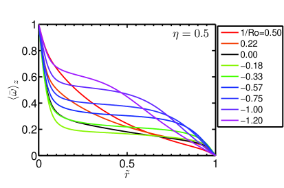
(a)

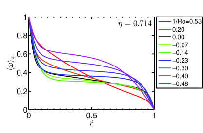
(b)

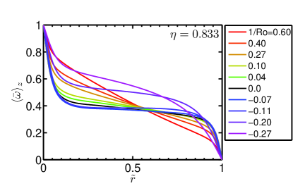
(c)

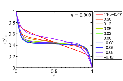
(d)

Figure 11: Azimuthally, axially and temporally averaged angular velocity $\langle\mathrm{bar}{\omega}\rangle_{z}$ versus radius $\tilde{r}$ for: $\eta=0.5$, $\eta=0.714$, $\eta=0.833$, and $\eta=0.909$. Data is for $Ta=2.5\cdot 10^{7}$ ($Ta=2.39\cdot 10^{7}$ for $\eta=0.714$) and selected values of $Ro^{-1}$. For smaller $\eta$, the $\omega$-bulk profiles differ more from a straight line, and have, on average, a smaller value.

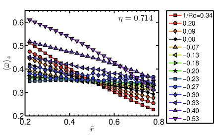
(a)

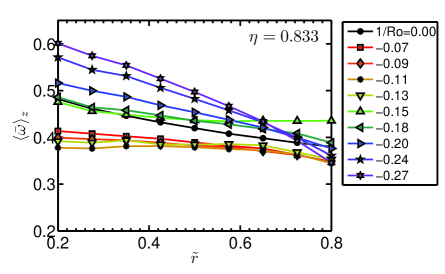
(b)

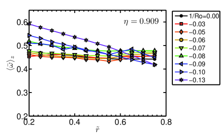
(c)

Figure 12: Angular velocity profiles obtained by LDA for $\eta=0.714$ at either $Re_{i}-Re_{o}=10^{6}$ (top), $\eta=0.833$ or at $Ta=5\cdot 10^{11}$ (bottom-left) and $\eta=0.909$ at $Ta=1.1\cdot 10^{11}$ (bottom-right), to explore different dependencies in parameter space. Data is taken at a fixed axial height (ie. the cylinder mid-height, $z=L/2$), but as the Taylor number $Ta$ is much larger than in the numerics, the axial dependence is much weaker.

5.2 Angular velocity profiles in the bulk

We now analyze the properties of the angular velocity profiles in the bulk. We find that the slope of the profiles in the bulk is controlled mainly by $Ro^{-1}$ and less so by $Ta$. This can be understood as follows: The Taylor number $Ta$ acts through the viscous term, dominant in the boundary layers, while $Ro^{-1}$ acts through the Coriolis force, present in the whole domain. These results extend the finding from Ostilla et al. (2013) to other values of $\eta$.

To further quantify the effect of $Ro^{-1}$ on the bulk profiles, we calculate the gradient of $\langle\mathrm{bar}{\omega}\rangle_{z}$. For the DNS data, this is done by numerically fitting a tangent line to the profile at the inflection point using the two neighboring points on both sides (at a distance of $0.01-0.02$ r-units); such fit is shown in the left panel of figure 13.

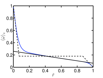
(a)

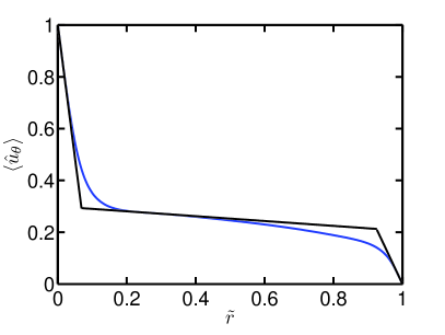
(b)

Figure 13: An example of the two fitting procedures for the bulk angular velocity gradient and for boundary layer thicknesses done on the DNS data is shown here. Both panels show the $\theta$,$z$, and $t$ averaged azimuthal velocity and angular velocity for $\eta=0.5$, $Ta$=$1\cdot 10^{7}$, and pure inner cylinder rotation. In the left panel a line is fitted to the bulk of the angular velocity to obtain the bulk gradient. The dashed lines indicate the EGL approximation. The right panel shows the three-lines-fit to the whole profile to obtain the width of its boundary layers, used in Section 5.3. Both bulk fits are done at the inflection point, but for different variables ($\mathrm{bar}{\omega}$ or $\mathrm{bar}{u}_{\theta}$), which gives slightly different slopes (and intersection points).

As the spatial resolution of the LDA data is more limited, the fit is done differently. A linear regression to the $\omega$-profile between $0.2<\tilde{r}<0.8$ is done. The larger range of $\tilde{r}$ is chosen in experiments because: (i) the boundary layers are small enough due to the high $Ta$ that they are outside of the fitting range, and (ii) the fluctuations of the data are much higher in experiments, especially for the LDA of the narrow gaps ($\eta=0.833$ and $\eta=0.909$). From this regression, we calculate $\langle\mathrm{bar}{\omega}\rangle_{z}$, and an error taken from the covariance matrix of the fit.

Figure 14 shows four panels, each containing the angular velocity gradient in the bulk from the numerical simulations and experiments for a given value of $\eta$. We first notice that the angular velocity gradients from experiment and numerics are in excellent agreement. Next the connection between a flat angular velocity profile and optimal transport for the highest drivings explored in the experiments can now be seen for other values of $\eta$ and not just for $\eta=0.714$ as reported previously (van Gils et al., 2011b). Once $Ro^{-1}<Ro^{-1}_{opt}$, the large scale balance analyzed in Ostilla et al. (2013) breaks down, and a “neutral” surface which reduces the transport appears in the flow.

In simulations, because of resolution requirements, we are unable of driving the flow strongly enough to see a totally flat bulk profile. Also, the influence of the large scale structures causes a small discrepancy between the flattest profile and the value of $Ro^{-1}_{opt}$ measured from $Nu_{\omega}$. This is expected to slowly dissapear with increasing $Ta$.

In Ostilla et al. (2013), a linear extrapolation of the bulk angular velocity gradient was done to give an estimate for the case when this profile would become horizontal, i.e., $d\langle\mathrm{bar}{\omega}\rangle_{z}/d\tilde{r}=0$, and thus give an estimate of $Ro^{-1}_{opt}$. For $\eta=0.714$ this estimate agreed with the numerical result within error bars. Here, we extend this analysis for the other values of $\eta$ and, as we shall see, successfully.

As in Ostilla et al. (2013), an almost linear relationship between $Ro^{-1}$ and $d\langle\mathrm{bar}{\omega}\rangle_{z}/d\tilde{r}$ can be seen. This linear relationship is extrapolated and plotted in each panel. This extrapolation gives an estimate for $Ro^{-1}_{opt}(Ta\to\infty)$, which we can compare to the experimentally determined $Ro^{-1}_{opt}(Ta\to\infty)$. For $\eta=0.833$, $Ro^{-1}(Ta\to\infty)\approx-0.12$ corresponding to $a\approx 0.38$ is obtained, and for $\eta=0.909$, $Ro^{-1}(Ta\to\infty)\approx-0.05$, corresponding to $a\approx 0.31$ is obtained. These values are (within error bars) also obtained for $Ro^{-1}_{opt}$ at the large $Ta$ investigated in experiments, namely $Ro^{-1}_{opt}=-0.10$ and $-0.05$, respectively.

For $\eta=0.5$, $Ro^{-1}_{opt}(Ta\to\infty)\approx-0.33$ is obtained, corresponding to $a\approx 0.2$. This value is consistent with the numerical results in Brauckmann & Eckhardt (2013b), which report $a_{opt}\approx 0.2$. However, care must be taken, as fitting straight lines to the $\omega$-profiles gives higher residuals for $\eta=0.5$ as the profiles deviate from straight lines (cf. top-left panel of figure 11). A fit to the “quarter-Couette” profile derived from upper bound theory (Busse, 1967) is much more appropriate for $\eta=0.5$ at the strongest drivings achieved in experiments (Merbold et al., 2013). This is because the flow feels much more the effect of the curvature at the small $\eta$. On the other end of the scale, the linear relationship works best for smallest gaps, i.e. $\eta=0.909$ (cf. the bottom right panel of figure 11) where curvature plays a small effect.

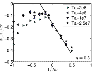
(a)

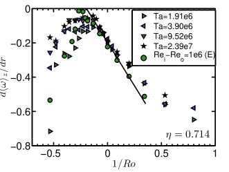
(b)

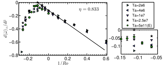
(c)

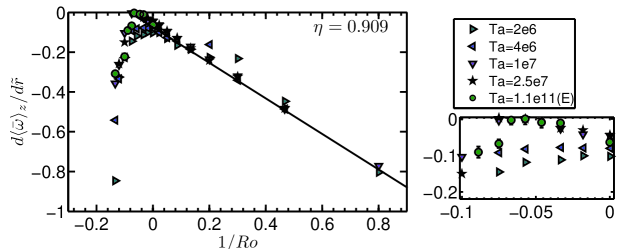
(d)

Figure 14: Bulk angular velocity gradient $d\langle\mathrm{bar}{\omega}\rangle_{z}/d\tilde{r}$ against $Ro^{-1}$ for the four values of $\eta$ explored in simulations, $\eta=0.5$ (top left), $\eta=0.714$, (top right), $\eta=0.833$, (middle), and $\eta=0.909$ (bottom). Data from experiments obtained by LDA is also plotted for the three values of $\eta$ for which it was experimentally measured (green circles). For all values of $\eta$ except $\eta=0.5$, for co–rotation and slight counter–rotation there is once again an almost linear relationship between $Ro^{-1}$ and $d\langle\mathrm{bar}{\omega}\rangle_{z}/d\tilde{r}$. A black straight line is added to extrapolate this relationship in order to estimate $Ro^{-1}_{opt}$. A plateau, in which the radial gradient of $\langle\mathrm{bar}{\omega}\rangle_{z}$ is small can be seen around optimal transport, indicating a large convective transport of angular velocity.

To further elaborate the link between $\eta$, flat $\omega$-profiles and $Ro^{-1}$, data for the smallest gap $\eta=0.95$ from Wendt (1933) has been digitized, and $d\langle\mathrm{bar}{\omega}\rangle_{z}/d\tilde{r}$ was been determined for it. This data corresponds to a driving of $Ta\sim 10^{8}-10^{9}$. Figure 15 shows $d\langle\mathrm{bar}{\omega}\rangle_{z}/d\tilde{r}$ against $Ro^{-1}$ for Wendt’s data and also for the current experimental data. The flattest profile can be seen to occur for increasing (in absolute value) $Ro^{-1}$ for larger gaps, simular to the shift of $Ro^{-1}$. For $\eta=0.95$, almost no curvature is felt by the flow and a flat profiles can be seen for $-0.05<Ro^{-1}<0$. However, adding a Coriolis force (in the form of $Ro^{-1}$) a large $\omega$-gradient is sustained in the bulk. This corroborates the balance between $Ro^{-1}$ and the bulk $\omega$-gradients proposed in Ostilla et al. (2013).

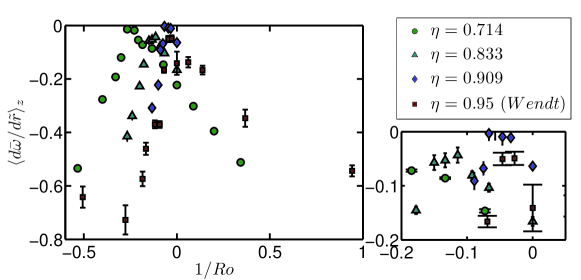
Figure 15: Bulk angular velocity gradient $d\langle\mathrm{bar}{\omega}\rangle_{z}/d\tilde{r}$ against $Ro^{-1}$ for the three values of $\eta$ explored in experiments, and for $\eta=0.95$ (digitized from Wendt (1933)). The error bars of Wendt’s data are larger due to the quality of the digitization. As seen previously, the flattest profile occurs around weak counter-rotation, for all values of $\eta$ including $\eta=0.95$.

5.3 Angular velocity profiles in the boundary layers in the classical turbulent regime

As the driving is increased, the transport is enhanced. To accommodate for this, the boundary layers (BLs) become thinner and therefore the $\omega$-slopes ($\partial_{r}\omega$) become steeper. Due to the geometry of the TC system an intrinsic asymmetry in the BL layer widths is present. More precisely, the exact relationship $\partial_{r}\langle\omega\rangle|_{o}=\eta^{3}\partial_{r}\langle\omega\rangle|_{i}$ holds for the slopes of the boundary layers, due to the $r$ independence of $J^{\omega}$, cf. EGL 2007 and eq.(6).

An analysis of the boundary layers was not possible in the present experiments because the present LDA measurements have insufficient spatial resolution to resolve the flow in the near–wall region. Therefore, only DNS results will be analyzed here. In simulations the driving is not as large as in experiments, and as a consequence the shear in the BLs is expected to not be large enough to cause a shear-instability. This means that the BLs are expected to be of Prandtl-Blasius (i.e. laminar) type, even if the bulk is turbulent. On the other hand, in the experiments both boundary layers and bulk are turbulent, i.e. the system is in the “ultimate regime”.

Using the DNS data, we can compare the ratio of the numerically obtained boundary layer widths with the analytical formula for this ratio obtained by EGL 2007 for laminar boundary layers, namely:

$$\frac{\lambda^{o}_{\omega}}{\lambda^{i}_{\omega}}=\eta^{-3}\displaystyle\frac{|\omega_{o}-\omega_{bulk}|}{|\omega_{i}-\omega_{bulk}|},$$ (14)

where the value of $\omega_{bulk}$ is some appropriate value in between for which the angular velocity at the inflection point of the profile might be chosen, i.e., the point at which the linear bulk profile fit was done to obtain $\lambda^{o}_{\omega}$ and $\lambda^{i}_{\omega}$. The value $\omega_{bulk}$ is taken from the numerics, and may bias the estimate.

To calculate the boundary layer thicknesses, the profile of the mean azimuthal velocity $\langle\mathrm{bar}{u}_{\theta}\rangle_{z}$ is approximated by three straight lines, one for each boundary layer and one for the bulk. For the boundary layers the slope of the fit is calculated by fitting (by least-mean-squares) a line through the first two computational grid points. For the bulk, first the line is forced to pass through the grid point which is numerically closest to the inflection point of the profile. Then its slope is taken from a least mean square fit using two grid points on both sides of this inflection point. The respective boundary layer line will cross with this bulk line at a point which then defines the thickness of that boundary layer.

The results obtained for $\lambda^{o}_{\omega}/\lambda^{i}_{\omega}$ both from equation 14 and directly from the simulations is shown in figure 14. Results are presented for the four values of $\eta$ and only for the highest value of $Ta$ achieved in the simulations. The boundary layer asymmetry for counter–rotating cylinders (i.e., $Ro^{-1}<0$) grows with larger gaps. This is to be expected, as the $\eta^{-3}$ term is much larger ($\approx 8$) for the largest gap as compared to the smallest gap ($\approx 1.3$). This is consistent with the $\eta$ and thus $\sigma$ restriction in EGL 2007 to a range of smaller gap widths.

As noticed already in Ostilla et al. (2013) we find that the fit is not satisfactory for co–rotation (i.e., $Ro^{-1}>0$) at the lowest values of $\eta$, but is satisfactory for counter–rotation (ie. $Ro^{-1}<0$). In EGL 2007, equation (14) is obtained by approximating the profile by three straight lines, two for the BLs and a constant $\omega$ line for the bulk. Therefore, we expect the approximation to hold best when the bulk has a flat gradient. For co–rotating cylinders and strongly counter–rotating cylinders, the bulk has a steep gradient (see figure 14), but characteristically different shapes. The only free parameter in equation (14) is $\omega_{bulk}$, which is chosen to be $\omega$ at the point of inflection. Due to the different shapes of the $\omega$-profiles, this choice seems more correct for counter-rotating cylinders, as there is a clear inflection point in the profile. On the other hand, for co-rotating cylinders, the profile appears to be more convex-like, and there, the choice of $\omega_{bulk}$ as the inflection point induces errors in the approximation (cf. 13a). For $\eta=0.5$, the error from the constant $\omega$ approximation is even more pronounced, and the formula fails.

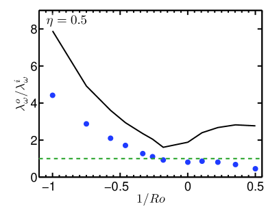
(a)

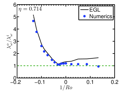
(b)

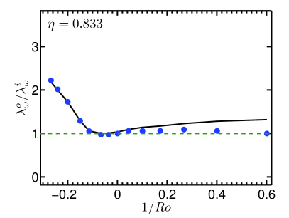
(c)

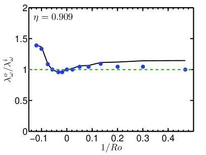
(d)

Figure 16: $\lambda^{o}_{\omega}/\lambda^{i}_{\omega}$ from simulations (dots) and from equation (14) (solid lines) versus $Ro^{-1}$ for the four values of $\eta$ studied numerically, $\eta=0.5$ (top-left), $0.714$ (top-right), $0.833$ (bottom-left) and $0.909$ (bottom-right) at $Ta=2.5\cdot 10^{7}$. The numerical results and the estimate from equation (14) match very well for larger values of $\eta$ and especially for counter–rotating cylinders ($1/Ro<0$). The asymmetry between the boundary layers can be seen to be larger for smaller values of $\eta$, which is expected as equation (14) contains the explicit factor $\eta^{-3}$.

For co–rotation the boundary layers are approximately of the same size, and the ratio $\lambda^{o}_{\omega}/\lambda^{i}_{\omega}$ is very close to $1$. If one inverts equation (14) by aproximating this ratio by $1$, an estimate of what the angular velocity will be in the bulk due to the boundary layer slope asymmetry is obtained:

$$\omega_{bulk}=\displaystyle\frac{\eta^{3}}{1+\eta^{3}},$$ (15)

corresponding to:

$$\omega^{\ell}_{bulk}=\displaystyle\frac{-\omega^{\ell}_{o}+\eta^{3}\omega_{i}^{\ell}}{1+\eta^{3}},$$ (16)

in the lab frame. This expression gives an estimate for $\omega_{bulk}$ when the profile is flattest, and has been represented graphically in figure 11. Indeed, one can take this estimate (for example $0.27$ for $\eta=0.714$) and compare it with figures 11 and 12. We note that the value of $\omega$ in the bulk for the flattest profile in the numerics (at $Ro^{-1}\approx Ro^{-1}_{opt}(Ta)$) lies around $\omega_{bulk}$. We can also notice that the profiles for $Ro^{-1}>Ro^{-1}_{opt}$ approximately cross each other at the same point, and this point has a value of $\omega\approx\omega_{bulk}$. This effect can only be seen in the numerics, as these approximations break down once the boundary layers become turbulent. The cross points of the curves are taken as an estimate for $\omega_{bulk}$, and this is represented against eq. 15 in figure 17.

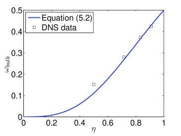
Figure 17: $\omega_{bulk}$ as a function of $\eta$, taken from both eq. 15 and from the crosspoints of the $\omega$-profiles in figure 11. The trend is the same in both data sets. A smaller value of $\eta$ decreases the value of the bulk angular velocity.

To understand why the boundary layers are of approximately the same thickness despite the different initial slopes at the cylinders one has to go back to equation (6). The angular velocity current has a diffusive part and a convective part. Per definition in the boundary layer the diffusion dominates and in the bulk the convection does. Thus the boundary layer ceases when convection becomes significant. But convection is controlled by the wind. Thus in essence the boundary layer size is controlled by the wind and not immediately by the initial slope at the wall. Due to continuity, if the rolls penetrate the whole domain the wind may be expected to be the same close to the inner and close to the outer cylinder. This suggests that the flow organizes itself in a way that the boundary layer extensions (or widths) might be similar, even if the initial slopes at the walls are different.

What happens for counter–rotation, or more precisely when $Ro^{-1}<Ro^{-1}_{opt}$? For $Ro^{-1}$ below the optimum $Ro^{-1}_{opt}$ a so-called neutral surface will be present in the flow, which separates the Rayleigh-stable and -unstable areas. The wind drastically changes in the Rayleigh-stable areas (Ostilla et al., 2013), leading to very different wind velocities close to the outer and inner cylinder, respectively. The wind at the outer cylinder will be weaker, as the rolls cannot fully penetrate the Rayleigh-stable domain. This means that the outer cylinder boundary layer will extend deeper into the flow, in accordance to what is seen in figure 16.

6 Summary and conclusions

Experiments and direct numerical simulations (DNS) were analysed to explore the effects of the radius ratio $\eta$ on turbulent Taylor-Couette flow. Numerical results corresponding to Taylor numbers in the range of $10^{4}<Ta<10^{8}$ alongside with experiments in a Taylor number range of $10^{10}<Ta<10^{12}$ were presented for four values of the radius ratio $\eta$.

First the influence of the radius ratio on the global scaling laws $Nu_{\omega}\sim Ta^{\gamma}$ was studied. The local scaling exponent $\gamma$ describing the response of the torque caused by a Taylor number increase, is barely modified by varying the radius ratio $\eta$. Indeed, in experiments a universal exponent of $\gamma\approx 0.39$ is obtained, independent of radius ratio and outer cylinder rotation. For the numerical simulations at lower $Ta$ similar universal behavior can be observed. The transition associated to the vanishing of coherent structures can also be appreciated at $Ta\sim 10^{6}$ for all values of $\eta$. Before this transition local exponents of $\gamma\approx 0.33$ are seen and after the transition these decrease to about $\gamma\approx 0.2$.

The radius ratio does play a very important role in optimal transport. At smaller gaps, i.e., for larger $\eta$, at the lower end of the $Ta$ range a very large increase in transport for corotating cylinders can be seen. The shift towards the asymptotic optimal transport happens in a much slower way for small gaps, but this shift is seen for all studied radius ratios. For the largest gap ($\eta=0.5$), optimal transport for pure inner cylinder rotation at the lowest drivings is obtained. The shift towards the asymptotic value happens suddenly, as two peaks can be seen in the $Nu_{\omega}$ versus $Ro^{-1}$ curve, and one of the peaks becomes larger than the other one as driving increases. This might point in the direction of different phenomena and transitions in the flow topology happening at larger gaps. Finally, the asymptotic values of $Ro^{-1}_{opt}$ obtained in experiments were compared to the speculation of van Gils et al. (2012) and the prediction of Brauckmann & Eckhardt (2013b). Both of the models were found to deviate from experimental and numerical results.

When looking at the local results, as in Ostilla et al. (2013) we can link the optimal transport in the smallest gaps to a balance between Coriolis forces and the inertia terms in the equations of motion. The flattest profiles in the bulk are linked to optimal transport in experiments. With the numerics the extrapolation presented in Ostilla et al. (2013) for predicting optimal transport was extended to other radius ratios. It is found to work well for all selected $\eta$ except for $\eta=0.5$. At this $\eta$, i.e., for the largest gap considered here, the most obvious problem is that the $\omega$ profiles strongly feel the effect of curvature difference at the inner and outer cylinders and a straight line fit to the bulk is not appropriate. There may be additional reasons for this discrepancy and optimal transport in large gaps requires more investigation. A summary of the results for determining $Ro^{-1}_{opt}$ using both the experimentally measured torque maxima from section 4.2 and the numerical extrapolation from section 5.2 are presented in table 2.

Radius ratio ($\eta$)	$Ro^{-1}_{opt}$/$a_{opt}$ from extrapolation	Measured $Ro^{-1}_{opt}$/$a_{opt}$
0.5	-0.33/0.20	-/-
0.714	-0.20/0.33	-0.20/0.33
0.769	-/-	-0.20/0.36
0.833	-0.12/0.41	-0.10/0.37
0.909	-0.05/0.34	-0.05/0.34

Table 2: Summary of values obtained for $Ro^{-1}_{opt}$ and $a_{opt}$ through both the extrapolation of $d\langle\mathrm{bar}{\omega}\rangle_{z}/d\tilde{r}$ (Section 5.2) and direct measurement of the torque (Section 4.2) for the various values of $\eta$ studied in this paper.

Finally, the boundary layers have been analyzed. The outer boundary layer is found to be much thicker than the inner boundary layer when $Ro^{-1}<Ro^{-1}_{opt}$. We attribute this to the appearance of Rayleigh-stable zones in the flow. This prevents the turbulent Taylor vortices from covering the full domain between the cylinders. As the boundary layer size is essentially determined by the wind, if the rolls penetrate the whole domain (which is the case for $Ro^{-1}>Ro^{-1}_{opt}$), both boundary layers are approximately of the same size. If the rolls do not penetrate the full domain, the outer boundary layer will be much larger than the inner boundary layer, in accordance with the smaller initial slope of $\omega(r)$ at the cylinder walls.

In this work, simulations and experiments have been performed on a range of radius ratios between $0.5\leq\eta\leq 0.909$. Insights for the small gaps seem to be consistent with what was discussed in Ostilla et al. (2013). However, for $\eta=0.5$ the phenomena of optimal transport appears to be quite different. Therefore, our ambition is to extend the DNS towards values of $\eta$ smaller than $0.5$ to improve the understanding of that regime.

Acknowledgements: We would like to thank H. Brauckmann, B. Eckhardt, S. Merbold, M. Salewski, E. P. van der Poel and R. C. A. van der Veen for various stimulating discussions during these years, and G.W. Bruggert, M. Bos and B. Benschop for technical support. We acknowledge that the numerical results of this research have been achieved using the PRACE-2IP project (FP7 RI-283493) resource VIP based in Germany at Garching. We would also like to thank the Dutch Supercomputing Consortium SurfSARA for technical support and computing resources. We would like to thank FOM, the Simon Stevin Prize of the Technology Foundation STW of The Netherlands, COST from the EU and ERC for financial support through an Advanced Grant.

References

- Ahlers (1974) Ahlers, G. 1974 Low temperature studies of the Rayleigh-Bénard instability and turbulence. Phys. Rev. Lett. 33, 1185–1188.
- Ahlers et al. (2009) Ahlers, G., Grossmann, S. & Lohse, D. 2009 Heat transfer and large scale dynamics in turbulent Rayleigh-Bénard convection. Rev. Mod. Phys. 81, 503.
- Andereck et al. (1986) Andereck, C. D., Liu, S. S. & Swinney, H. L. 1986 Flow regimes in a circular couette system with independently rotating cylinders. J. Fluid Mech. 164, 155.
- Behringer (1985) Behringer, R. P. 1985 Rayleigh-Bénard convection and turbulence in liquid-helium. Rev. Mod. Phys. 57, 657 – 687.
- Benjamin (1978) Benjamin, T. B. 1978 Bifurcation phenomena in steady flows of a viscous liquid. Proc. R. Soc. London A 359, 1–43.
- Bodenschatz et al. (2000) Bodenschatz, E., Pesch, W. & Ahlers, G. 2000 Recent developments in Rayleigh-Bénard convection. Ann. Rev. Fluid Mech. 32, 709–778.
- Brauckmann & Eckhardt (2013a) Brauckmann, H. & Eckhardt, B. 2013a Direct numerical simulations of local and global torque in Taylor-Couette flow up to Re=30.000. J. Fluid Mech. 718, 398–427.
- Brauckmann & Eckhardt (2013b) Brauckmann, H. & Eckhardt, B. 2013b Intermittent boundary layers and torque maxima in Taylor-Couette flow. Phys. Rev. E 87, 033004.
- Busse (1967) Busse, F. H. 1967 The stability of finite amplitude cellular convection and its relation to an extremum principle. J. Fluid Mech. 30, 625–649.
- Chandrasekhar (1981) Chandrasekhar, S. 1981 Hydrodynamic and Hydromagnetic Stability. New York: Dover.
- Couette (1890) Couette, M. 1890 Études sur le frottement des liquides. Gauthier-Villars et fils.
- Coughlin & Marcus (1996) Coughlin, K. & Marcus, P. S. 1996 Turbulent bursts in Couette-Taylor flow. Phys. Rev. Lett. 77 (11), 2214–17.
- Cross & Hohenberg (1993) Cross, M. C. & Hohenberg, P. C. 1993 Pattern formation outside of equilibrium. Rev. Mod. Phys. 65 (3), 851.
- Dominguez-Lerma et al. (1986) Dominguez-Lerma, M. A., Cannell, D. S. & Ahlers, G. 1986 Eckhaus boundary and wavenumber selection in rotating Couette-Taylor flow. Phys. Rev. A 34, 4956.
- Dong (2007) Dong, S 2007 Direct numerical simulation of turbulent taylor-couette flow. J. Fluid Mech. 587, 373–393.
- Dong (2008) Dong, S 2008 Turbulent flow between counter-rotating concentric cylinders: a direct numerical simulation study. J. Fluid Mech. 615, 371–399.
- Donnelly (1991) Donnelly, R. 1991 Taylor-Couette flow: the early days. Physics Today pp. 32–39.
- Drazin & Reid (1981) Drazin, P.G. & Reid, W. H. 1981 Hydrodynamic stability. Cambridge: Cambridge University Press.
- Eckhardt et al. (2007) Eckhardt, B., Schneider, T.M., Hof, B. & Westerweel, J. 2007 Turbulence transition in pipe flow. Annu. Rev. Fluid Mech. 39, 447–468.
- Esser & Grossmann (1996) Esser, A. & Grossmann, S. 1996 Analytic expression for Taylor-Couette stability boundary. Phys. Fluids 8, 1814–1819.
- Fasel & Booz (1984) Fasel, H. & Booz, O. 1984 Numerical investigation of supercritical taylor-vortex flow for a wide gap. J. Fluid Mech. 138, 21–52.
- Gebhardt & Grossmann (1993) Gebhardt, Th. & Grossmann, S. 1993 The Taylor-Couette eigenvalue problem with independently rotating cylinders. Z. Phys. B 90 (4), 475–490.
- van Gils et al. (2011a) van Gils, D. P. M., Bruggert, G. W., Lathrop, D. P., Sun, C. & Lohse, D. 2011a The Twente Turbulent Taylor-Couette () facility: strongly turbulent (multi-phase) flow between independently rotating cylinders. Rev. Sci. Instr. 82, 025105.
- van Gils et al. (2011b) van Gils, D. P. M., Huisman, S. G., Bruggert, G. W., Sun, C. & Lohse, D. 2011b Torque scaling in turbulent Taylor-Couette flow with co- and counter-rotating cylinders. Phys. Rev. Lett. 106, 024502.
- van Gils et al. (2012) van Gils, D. P. M., Huisman, S. G., Grossmann, S., Sun, C. & Lohse, D. 2012 Optimal Taylor-Couette turbulence. J. Fluid Mech. 706, 118.
- Grossmann & Lohse (2000) Grossmann, S. & Lohse, D. 2000 Scaling in thermal convection: A unifying view. J. Fluid. Mech. 407, 27–56.
- Grossmann & Lohse (2001) Grossmann, S. & Lohse, D. 2001 Thermal convection for large Prandtl number. Phys. Rev. Lett. 86, 3316–3319.
- Grossmann & Lohse (2011) Grossmann, S. & Lohse, D. 2011 Multiple scaling in the ultimate regime of thermal convection. Phys. Fluids 23, 045108.
- Grossmann & Lohse (2012) Grossmann, S. & Lohse, D. 2012 Logarithmic temperature profiles in the ultimate regime of thermal convection. Phys. Fluids 24, 125103.
- Huisman et al. (2012a) Huisman, S.G., van Gils, D.P.M. & Sun, C. 2012a Applying laser doppler anemometry inside a taylor-couette geometry – using a ray-tracer to correct for curvature effects. Eur. J. Mech. - B/Fluids 36, 115–119.
- Huisman et al. (2012b) Huisman, S. G., van Gils, D. P. M., Grossmann, S., Sun, C. & Lohse, D. 2012b Ultimate turbulent Taylor-Couette flow. Phys. Rev. Lett. 108, 024501.
- Huisman et al. (2013) Huisman, S. G., Scharnowski, S., Cierpka, C., Kaehler, C., Lohse, D. & Sun, C. 2013 Logarithmic boundary layers in highly turbulent Taylor-Couette flow. Phys. Rev. Lett 110, 264501.
- Kadanoff (2001) Kadanoff, L. P. 2001 Turbulent heat flow: Structures and scaling. Phys. Today 54 (8), 34–39.
- Lathrop et al. (1992a) Lathrop, D. P., Fineberg, Jay & Swinney, H. S. 1992a Transition to shear-driven turbulence in Couette-Taylor flow. Phys. Rev. A 46, 6390–6405.
- Lathrop et al. (1992b) Lathrop, D. P., Fineberg, Jay & Swinney, H. S. 1992b Turbulent flow between concentric rotating cylinders at large Reynolds numbers. Phys. Rev. Lett. 68, 1515–1518.
- Lewis & Swinney (1999) Lewis, G. S. & Swinney, H. L. 1999 Velocity structure functions, scaling, and transitions in high-Reynolds-number Couette-Taylor flow. Phys. Rev. E 59, 5457–5467.
- Lohse & Xia (2010) Lohse, D. & Xia, K.-Q. 2010 Small-scale properties of turbulent Rayleigh-Bénard convection. Ann. Rev. Fluid Mech. 42, 335–364.
- Lorenz (1963) Lorenz, E. N. 1963 Deterministic nonperiodic flow. J. Atmos. Sci 20, 130–141.
- Mallock (1896) Mallock, A. 1896 Experiments on fluid viscosity. Phil. Trans. R. Soc. Lond. A 187, 41–56.
- Merbold et al. (2013) Merbold, S., Brauckmann, H. & Egbers, C. 2013 Torque measurements and numerical determination in differentially rotating wide gap Taylor-Couette flow. Phys. Rev. E 87, 023014.
- Ostilla et al. (2013) Ostilla, R., Stevens, R. J. A. M., Grossmann, S., Verzicco, R. & Lohse, D. 2013 Optimal Taylor-Couette flow: direct numerical simulations. J. Fluid Mech. 719, 14–46.
- Ostilla Monico et al. (2013) Ostilla Monico, R., van der Poel, E., Verzicco, R., Grossmann, S. & Lohse, D. 2013 Boundary layer dynamics at the transition between the classical and the ultimate regime of Taylor-Couette flow. submitted to Physics of Fluids .
- Paoletti & Lathrop (2011) Paoletti, M. S. & Lathrop, D. P. 2011 Angular momentum transport in turbulent flow between independently rotating cylinders. Phys. Rev. Lett. 106, 024501.
- Pfister & Rehberg (1981) Pfister, G. & Rehberg, I. 1981 Space dependent order parameter in circular Couette flow transitions. Phys. Lett. 83, 19–22.
- Pfister et al. (1988) Pfister, G, Schmidt, H, Cliffe, K A & Mullin, T 1988 Bifurcation phenomena in Taylor-Couette flow in a very short annulus. J. Fluid Mech. 191, 1–18.
- Pirro & Quadrio (2008) Pirro, Davide & Quadrio, Maurizio 2008 Direct numerical simulation of turbulent Taylor-Couette flow. Eur. J. Mech. B-Fluids 27, 552.
- Siggia (1994) Siggia, E. D. 1994 High Rayleigh number convection. Annu. Rev. Fluid Mech. 26, 137–168.
- Smith & Townsend (1982) Smith, G. P. & Townsend, A. A. 1982 Turbulent Couette flow between concentric cylinders at large Taylor numbers. J. Fluid Mech. 123, 187–217.
- Stevens et al. (2011) Stevens, R. J. A. M., Lohse, D. & Verzicco, R. 2011 Prandtl and Rayleigh number dependence of heat transport in high Rayleigh number thermal convection. J. Fluid Mech. 688, 31–43, submitted.
- Stevens et al. (2010) Stevens, R. J. A. M., Verzicco, R. & Lohse, D. 2010 Radial boundary layer structure and Nusselt number in Rayleigh-Bénard convection. J. Fluid Mech. 643, 495–507.
- Strogatz (1994) Strogatz, S. H. 1994 Nonlinear dynamics and chaos. Reading: Perseus Press.
- Swinney & Gollub (1981) Swinney, H. L. & Gollub, J. P. 1981 Hydrodynamic instabilities and the transition to turbulence, , vol. 45 (Topics in Applied Physics). Berlin: Springer-Verlag.
- Taylor (1936) Taylor, G. I. 1936 Fluid friction between rotating cylinders. Proc. R. Soc. London A 157, 546–564.
- Tong et al. (1990) Tong, P., Goldburg, W. I., Huang, J. S. & Witten, T. A. 1990 Anisotropy in turbulent drag reduction. Phys. Rev. Lett. 65, 2780–2783.
- Verzicco & Orlandi (1996) Verzicco, R. & Orlandi, P. 1996 A finite-difference scheme for three-dimensional incompressible flow in cylindrical coordinates. J. Comput. Phys. 123, 402–413.
- Wendt (1933) Wendt, F. 1933 Turbulente Strömungen zwischen zwei rotierenden Zylindern. Ingenieurs-Archiv 4, 577–595.
- Xia et al. (2002) Xia, K.-Q., Lam, S. & Zhou, S. Q. 2002 Heat-flux measurement in high-Prandtl-number turbulent Rayleigh-Bénard convection. Phys. Rev. Lett. 88, 064501.