Spatially localized solutions of shear flows

Abstract

We present several new spatially localized equilibrium and traveling-wave solutions of plane Couette and channel flows. The solutions exhibit strikingly concentrated regions of vorticity that are flanked on either side by high-speed streaks. For several traveling-wave solutions of channel flow, the concentrated vortex structures are confined to the near-wall region and form particularly isolated and elemental versions of coherent structures in the near-wall region of shear flows. The solutions are constructed by a variety of methods: application of windowing functions to previously known spatially periodic solutions, continuation from plane Couette to channel flow conditions, and from initial guesses obtained from turbulent simulation data. We show how the symmetries of localized solutions derive from the symmetries of their periodic counterparts, analyze the exponential decay of their tails, examine the scale separation and scaling of their streamwise Fourier modes, and show that they develop critical layers for large Reynolds numbers.

1 Introduction

Over the last twenty years the computation of invariant solutions of the Navier-Stokes equations, or “exact coherent structures,” has opened a new approach to understanding the dynamics of moderate-Reynolds unsteady flows, an approach which promises to provide a long-hoped-for bridge between dynamical systems theory and turbulence. Unlike previous derivations of low-order dynamical models of unsteady flows (Lorenz (1963); Aubry et al. (1988); Holmes et al. (1996)), the invariant-solutions approach forgoes low-d projections and simplified models and instead takes a fully-resolved direct numerical simulation as a quantitatively accurate finite-dimensional approximation of the Navier-Stokes equations. The fully-resolved simulation is then treated as very high-dimensional dynamical system. The first step in analysis of a dynamical system is the computation of its invariant solutions: its equilibria, homo- and heteroclinic orbits, and periodic orbits. In the dynamical systems view of turbulence, the equilibrium solutions correspond to steady states of the fluid flow, periodic orbits correspond to states of the fluid velocity field repeat themselves exactly after a finite time, and homo- and heteroclinic orbits correspond to dynamic transitions between equilibria or periodic orbits. For flows with homogeneous spatial directions, such as pipes and channels, continuous symmetries in the equations of motion allow relative invariant solutions, e.g. traveling waves (relative equilibria) and relative periodic orbits.

The simplest invariant solutions of fluids are the classical, closed-form steady states of the Navier-Stokes equations, for example, the parabolic laminar flow profile of pressure-driven channel and pipe flow, or the linear laminar solution of plane Couette flow. Solutions such as these have special cancellations which make it possible to represent the exact solution of the nonlinear system with a finite set of simple functions. For example, for the laminar solution of channel flow, the nonlinear term vanishes and the solution can be represented exactly as a 2nd order polynomial in the wall-normal variable. However, if we consider the problem from the perspective of faithful, very high-dimensional finite discretizations, invariant solutions are the solutions of a nonlinear algebraic or differential equations in $O(10^{4})$ to $O(10^{6})$ free variables. Only a few very special solutions (the classical ones) will involve few enough modes to be expressible in closed form, and most will involve nonlinear coupling between large numbers of nonzero variables. Compared to the classical closed-form solutions, these computed invariant solutions are typically unstable, fully three-dimensional, fully nonlinear, distant from the smooth laminar flow solutions, and involve most if not all the available modes of the numerical representation. Determination and specification of such solutions is necessarily numerical.

The practical feasibility of finding such high-dimensional nonlinear solutions of Navier-Stokes was first demonstrated by Nagata (1990), who computed an unstable 3-dimensional nonlinear equilibrium solution of plane Couette flow at a Reynolds number above the onset of turbulence, using a 589-dimensional discretization. The same equilibrium solution was found independently and analyzed in greater precision and detail by Clever & Busse (1992) and Waleffe (1998, 2003). A large number of equilibria and traveling waves of plane Couette and pipe flow have since been found (Nagata (1997); Schmiegel (1999); Faisst & Eckhardt (2003); Gibson et al. (2009)), a few of channel flow (Waleffe (2001); Itano & Toh (2001)), and in other flows such square duct flow (Okino et al. (2010), Wedin & Kerswell (2009)). Periodic orbits have been calculated for plane Couette flow (Kawahara & Kida (2001); Viswanath (2007); Cvitanović & Gibson (2010)), pipe flow (Duguet et al. (2008)), and 2D Kolmogorov turbulence (Chandler & Kerswell (2013)), and hetero- and homoclinic connections for plane Couette flow (Gibson et al. (2008); Halcrow et al. (2009); van Veen & Kawahara (2011)). Improved numerical methods and more powerful computers now allow the computation of solutions with as many as $10^{6}$ free variables. High-resolution calculations have shown that discretization errors converge toward zero as resolution is increased, demonstrating that the numerical solutions are precise approximations of true solutions of the Navier-Stokes equations, rather than artifacts of discretization. High-resolution calculations have also allowed accurate computation of solutions with fine spatial structure, such as periodic orbits that exhibit turbulent “bursting” phases (Viswanath (2007); Cvitanović & Gibson (2010)).

Just as in low-dimensional dynamical systems theory, the importance of these invariant solutions stems from the organization they impose on the state space dynamics. In particular, dynamics in the neighborhood of (relative) equilibria and periodic orbits is governed to leading order by the linearization about these solutions, and the eigenvalues of the linearized dynamics reveal the local character of the state space flow and the dimensionality of each solution’s unstable manifold. For shear flows at moderate Reynolds numbers and in closed or small periodic domains, most known invariant solutions have a positive but remarkably small number of unstable eigenvalues, and correspondingly low-dimensional unstable manifolds. For example, the equilibrium solution of plane Couette flow developed by Nagata, Busse, Clever, and Waleffe (hereafter termed the NBCW equilibrium) has a single unstable eigenvalue (Wang et al. (2007), and the periodic orbit solutions of Viswanath (2007) have between 1 and 11 unstable eigenvalues. This low dimensionality of instability is a crucially important result. It suggests, as long suspected, that moderate-Reynolds flows are inherently low-dimensional –at least for small confined domains. It further suggests that the temporal dynamics of such flows results from a relatively low-dimensional, chaotic but deterministic walk between the flow’s unstable invariant solutions, along the low-dimensional network of their unstable manifolds (Gibson et al. (2008)). Moreover, the coherent structures often observed in such flows can be understood as resulting from close passes to these unstable invariant solutions, at which the Navier-Stokes equations balance exactly –an idea well-expressed by Waleffe’s term “exact coherent structures” (Waleffe (2001)). Indeed, a key feature of the NBCW invariant solution is that it captures structure commonly observed in shear flows in the form of wavy rolls that support alternating streaks of high and low streamwise velocity (see § 2.2 for further discussion). We refer the reader to the Kawahara et al. (2012) review article for an excellent overview of research in this area.

On the other hand, a significant weakness of the invariant-solutions approach to date is the assumption of idealized computational domains, for example, small periodic “minimal flow units” (Hamilton et al. (1995)), just large enough to contain a single coherent structure. For example, most of the work analyzing dynamics via invariant solutions has been done in plane Couette flow in doubly-periodic boxes with stream- and spanwise aspect ratios around 2 or 3. Small periodic or confined domains are an understandable simplifying assumption for the demanding computational problem of computing invariant solutions. However, it is also valid to criticize such assumptions as unphysical and limiting the research to explorations of temporal complexity of periodic spatial structures, as opposed to the full spatio-temporal complexity of turbulence in extended domains. The assumption of periodicity also complicates coordination of theory and experiment. Close passes to unstable traveling waves with axial periodicity have been have been detected in experimental pipe flows (Hof et al. (2004); de Lozar et al. (2012)), but the effort to match experiment and theory would be greatly aided if the assumption of periodicity in the computations could be relaxed. Lastly, the most prominent example of coherent structures in fluids, and the initial motivating problem for dynamical-systems approaches, are the lambda and hairpin vortices that form in the high-shear region near the walls of channel and boundary layer flows. These appear in coupled systems of coherent structures that are individually localized in the wall-normal direction as well as the two homogeneous directions (Adrian (2007)).

The first step in addressing the weakness of small, idealized domains is to compute localized invariant solutions on extended domains. Several papers have made promising steps in this direction. Schneider et al. (2009) computed the first spatially localized equilibrium and traveling waves of Navier-Stokes, by an “edge-tracking” algorithm for plane Couette flow in a streamwise-periodic but spanwise-extended domain, and showed that these solutions were spanwise-localized forms of the spatially periodic NBCW solution, which exhibit exponential decay towards laminar flow in the spanwise coordinate. Another computation in the same paper produced an unsteady, time-varying state with exponential localization in both span- and streamwise directions. However, this state appears to wander chaotically and so is not an invariant solution. A similar time-varying doubly-localized state was found by Duguet et al. (2009). Schneider et al. (2010) demonstrated a number of interesting connections between the localized solutions of Schneider et al. (2009) and localized solutions of the Swift-Hohenberg equation. Both systems exhibit homoclinic snaking, a process by which localized solutions grow additional structure at their fronts via a sequence of saddle-node bifurcations in a continuation parameter (see § 4.2 for further discussion). This is an intriguing connection, as Swift-Hohenberg is a key model equation in the theory of pattern formation (Hoyle (2006)), for which localization is comparatively well-understood (Burke & Knobloch (2007)).

The broad purposes of the present paper are (1) to further extend the invariant-solutions approach to turbulence to spatially extended flows, towards the long-term goals of addressing spatio-temporal complexity in turbulence and aiding the effort to verify invariant solutions in experiment, and (2) to begin an effort to capture spatially isolated coherent structures that occur near the walls of shear flows. The specific results and organization of the paper are as follows. In § 2 we show that the spanwise localized solutions of Schneider et al. (2010, 2009) are not anomalous, but that localized versions of other spatially periodic solutions exist and can be constructed easily by a windowing and refinement method that, unlike edge-tracking, puts no restrictions on the number of the solution’s unstable eigenmodes. We show how the symmetries of localized solutions result from the symmetries and phase of the underlying periodic solution. In § 3, to further develop the invariant-solutions approach in experimentally accessible flow conditions, we construct localized traveling wave solutions of channel flow, by windowing and refining periodic solutions obtained by continuation from plane Couette conditions and by searching among turbulent simulation data. In doing so we find particularly intriguing traveling-wave solutions of channel flow whose vorticity is concentrated in the near-wall region, in spanwise and wall-normal localized structures that resemble lambda vortices in streamwise-developing channel flows. In § 4 we analyze the tails of the localized solutions and show that they decay exponentially to laminar flow at the rate determined solely by the streamwise wavenumber of the solution, with far-field structure that is independent of the details of the core region. We examine scale separation and scaling in the streamwise Fourier harmonics and development of critical layers at large Reynolds numbers.

2 Equilibrium solutions of plane Couette flow

2.1 Equations of motion

Plane Couette flow consists of an incompressible fluid confined between two parallel rigid plates moving in-plane at a constant relative velocity. The ${\bf x}=(x,y,z)$ coordinates are aligned with the streamwise, wall-normal, and spanwise directions, where streamwise is defined as the direction of relative wall motion. We assume a computational flow domain $\Omega=[-L_{x}/2,\>L_{x}/2]\times[-h,h]\times[-L_{z}/2,\>L_{z}/2]$ with periodic boundary conditions in $x$ and $z$ and no-slip conditions at the walls $y=\pm h$. We restrict our attention to streamwise-periodic velocity fields and $L_{x}$ chosen to match the streamwise wavelength. In the spanwise direction, we choose $L_{z}$ either to match the spanwise wavelength of a spanwise periodic field, or to a large value that approximates a spanwise-infinite domain. We decompose the total velocity and pressure fields into sums of a laminar base flow and a deviation from laminar: ${\bf u}_{\text{tot}}({\bf x},t)={\bf u}({\bf x},t)+U(y)\,{\bf e}_{x}$ and $p_{\text{tot}}=p({\bf x},t)+x\;dP\!/\!dx$, where $dP\!/\!dx$ is a fixed constant specifying an imposed mean pressure gradient. For plane Couette flow we will consider only the case $dP\!/\!dx=0$, for which the laminar solution is $U(y)=\bar{U}y/h$, where $\bar{U}$ is half the relative wall speed. After nondimensionalization by $\bar{U}$, $h$, and the kinematic viscosity $\nu$, the Navier-Stokes equations for plane Couette flow can be written

$$\frac{\partial{\bf u}}{\partial t}+U\frac{\partial{\bf u}}{\partial x}+v\>U^{\prime}\>{\bf e}_{x}+{\bf u}\cdot{\bf\nabla}{\bf u}=-\nabla p+\frac{1}{Re}\nabla^{2}{\bf u},\quad\nabla\cdot{\bf u}=0$$ (1)

where $Re=\bar{U}h/\nu$ and the velocity components are ${\bf u}({\bf x},t)=[u,v,w](x,y,z,t)$. In this decomposition the plane Couette laminar solution is $U(y)=y$, $dP\!/\!dx=0$, ${\bf u}=0$, and $p=0$. From here on we refer to ${\bf u}$ as velocity and ${\bf u}_{\text{tot}}$ as total velocity, and we note that ${\bf u}$ has Dirichlet boundary conditions at the walls.

The Navier-Stokes equations (1) with plane Couette conditions and $y$-Dirichlet, $x,z$-periodic boundary conditions are invariant under any combination of rotation by $\pi$ about the $z$ axis, reflection about the $z=0$ plane, and finite translations in the $x$ and $z$ directions. The generators of the plane Couette symmetry group are thus

$$\sigma_{xy} :[u,v,w](x,y,z)\rightarrow[-u,-v,w](-x,-y,z)$$

$$\sigma_{z} :[u,v,w](x,y,z)\rightarrow[u,v,-w](x,y,-z)$$ (2)

$$\tau(\Delta x,\Delta z) :[u,v,w](x,y,z)\rightarrow[u,v,w](x+\Delta x,y,z+\Delta z).$$

We use the standard group-theory notation $\langle\ldots\rangle$ to indicate the group generated by a set of group elements; thus the symmetry group of plane Couette flow is $\langle\sigma_{xy},\sigma_{z},\tau(\Delta x,\Delta z)\rangle$. For each subgroup of this group, there is a subspace of velocity fields that is invariant under the equations of motion. That is, if a velocity field ${\bf u}({\bf x},0)$ satisfies ${\bf u}=\sigma{\bf u}$ for each symmetry $\sigma$ in a given subgroup, ${\bf u}({\bf x},t)$ will satisfy the same symmetries for all time. Invariant solutions of the equations of motion naturally lie in these subspaces. For example, with appropriate choice of the origin, equilibrium solutions of plane Couette typically satisfy $[u,v,w](x,y,z)=[-u,-v,-w](-x,-y,-z)$ or related symmetries involving $\sigma_{xy}$ and $\sigma_{z}$, since these symmetries requires the velocity field to vanish at the origin, and so prevent drifting in $x$ and $z$.

2.2 Spatially periodic solutions: EQ1/NBCW, EQ7/HSV, and EQ8

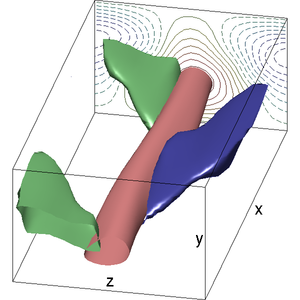
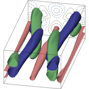
(a) (b) (c)

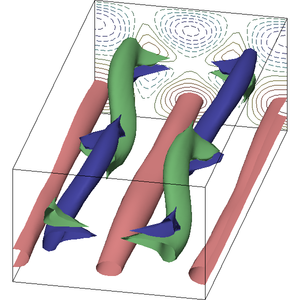
Figure 1: Three spatially periodic equilibria of plane Couette flow. (a) NBCW lower branch, (b) EQ7 lower branch, and (c) EQ8 (upper branch of EQ7), all at $Re=400$ and $\alpha,\gamma=1,2$, where $\alpha$ and $\gamma$ are the streamwise and spanwise wavenumbers. The visualizations show 3D isosurfaces of signed swirling strength at $s=\pm 0.09$ in green/blue (see text). Isosurfaces of streamwise velocity indicating high-speed streaks are shown in red at (a) $u=0.3$, (b) $u=0.15$, and (c) $u=0.2$. The back plane shows contours of streamwise velocity at levels (a,c) $\pm 0.03\cdot[1\!:2\!:15]$ and (b) $\pm 0.03\cdot[1\!:2\!:5]$ in Matlab notation with dashed/solid lines indicating negative/positive values. Note that by symmetry both solutions have streaks of equal magnitude and opposite streamwise velocity; these are not shown in the isosurfaces to reduce clutter, but they are indicated by the negative/positive symmetry of the backplane contours of streamwise velocity. The origin is at the center of the box.

Figure 1 shows a visualization of three spatially periodic equilibrium solutions of plane Couette flow: the well-known “lower branch” solution of Nagata (1990), Clever & Busse (1992), and Waleffe (1998) (NBCW, called EQ1 in Gibson et al. (2009))), and the “Hairpin Vortex Solution (HVS)” of Itano & Generalis (2009) and discovered independently as EQ7 in Gibson et al. (2009). Henceforth we refer to these as NBCW and EQ7. EQ8 is the upper branch of the the HSV/EQ7 solution. The NBCW solution is well-known not only as the first known exact nonlinear solution to the Navier-Stokes equations, but also for a number of remarkable characteristics, which we outline briefly here. The NBCW solution captures precisely, in the context of plane Couette flow, the roll-streak structure that seems ubiquitous in shear flows ranging from Taylor-Couette to the turbulent boundary layer, and consequently forms an example of an exact instantaneous balance between the three cycles of Waleffe’s self-sustaining process for shear flows (Waleffe (1997, 1998)). The NBCW solution has also served as a starting point for recent efforts to formulate a dynamical-systems theory of turbulence. At Reynolds numbers above the onset of turbulence, the NBCW solution lies between the laminar solution and the chaotic turbulent region of state space. It has a single unstable eigenvalue (Wang et al. (2007), so that its stable manifold forms a boundary between states that decay to laminar flow and states that grow to turbulence (Schneider et al. (2008)). The comparatively low viscous shear rate of the NBCW solution suggests that it might be feasible to implement a control strategy to stabilize this single unstable direction and obtain savings in the wall driving force compared to the turbulent flow (Wang et al. (2007)). The NBCW solution also has been shown to have well-defined asymptotic structure in the limit of large Reynolds number, which can be exploited to form a reduced system that accurately captures the structure of the solution over a wide range of Reynolds numbers (Wang et al. (2007); Hall & Sherwin (2010)). The asymptotic structure and reduced system are particularly relevant for this work, since it seems likely that any analytic understanding of localization in Navier-Stokes will be more easily developed in the context of a reduced system.

The EQ7 solution has been conjectured to be related to hairpin vortices frequently observed in the turbulent boundary layer (Itano & Generalis (2009)). The hairpin shapes in the visualizations of Itano & Generalis (2009) are certainly suggestive; however, some caution should be in order, as these visualizations of vortex lines cannot be compared directly to visualizations that highlight the magnitude of vorticity, such as Q criterion, lambda criterion, and swirling strength. Figure 1 shows NBCW, EQ7, and EQ8 visualized with signed swirling strength isosurfaces to show the roll structure and streamwise velocity isosurfaces to show high-speed streaks. The swirling strength at ${\bf x}$ is defined as the magnitude of the complex part of the eigenvalue of the velocity gradient tensor ${\bf\nabla}{\bf u}({\bf x})$ (Zhou et al. (1999)). We chose swirling strength over other measures of fluid circulation such as Q criterion because it most clearly identified in 3D isosurfaces the regions of highly concentrated circulation that are apparent in 2D quiver plots such figure 4. Since the invariant solutions in this paper have elongated regions of concentrated circulation nearly aligned with the $x$ axis, we attached a $\pm$ sign to the swirling strength that indicates clockwise/counterclockwise circulation with respect to the positive $x$ axis.

2.3 Construction of localized initial guesses by windowing

The localized equilibria and traveling waves of plane Couette flow described in Schneider et al. (2009) and Schneider et al. (2010) (hereafter SGB10) are spanwise-localized versions of the spatially periodic NBCW solution. These localized solutions are comprised of a core region that closely resembles the periodic NBCW solution, weak tails that decay exponentially towards laminar flow, and a transitional region between the core and tails. This form suggests that new localized solutions might be found by imposing a similar core-transition-tail structure on other known spatially periodic solutions, and then refining these initial guesses with a trust-region Newton-Krylov solver. The rough form of this desired structure can be imposed on initial guesses by multiplying a known spatially periodic solution, expressed as a perturbation on laminar flow, by an even positive windowing function $W(z)$ that is nearly unity over a core region $|z|<a$, decreases smoothly and monotonically to nearly zero over a transition region $a\leq|z|<a+b$, and vanishes as $|z|\rightarrow\infty$, followed by projecting the resulting field $W(z){\bf u}({\bf x})$ onto the divergence-free subspace. We have found that with a robust trust-region Newton-Krylov solver, the precise details of the windowing function and the projection are unimportant, and that the only important details are smoothness and the widths of the core and transition regions. One choice that suffices is the windowing function

$$W(z)=\frac{1}{4}\;\left(1+\tanh\left(\frac{6(a-z)}{b}+3\right)\right)\left(1+\tanh\left(\frac{6(a+z)}{b}+3\right)\right).$$ (3)

This $W(z)$ behaves as desired: it is even, smooth, monotonic in $|z|$, satisfies $0.995<W(z)<1$ for $|z|<a$ and $0<W(z)<0.005$ for $|z|>a+b$, and it approaches zero exponentially as $|z|\rightarrow\infty$. $W(z)$ is specified in this particular form because we found that the most important factor in producing a good initial guess was the size and location of the transition region, which are specified by the parameters $a$ and $b$. A sufficient projection is to apply $W(z)$ to the streamwise and spanwise components of velocity and reconstruct the wall-normal from the divergence-free condition. That is, let ${\bf u}=[u,v,w]$ be a $z$-periodic solution expressed as a perturbation over laminar flow. An initial guess for a $z$-localized solution ${\bf u}_{g}=[u_{g},v_{g},w_{g}]$ can be constructed by setting $u_{g}=Wu$, $w_{g}=Ww$, and reconstructing $v_{g}$ from ${\bf\nabla}\cdot{\bf u}_{g}=0$ and boundary conditions.

It is worth emphasizing that this localization procedure is rather crude. By construction, the initial guess should nearly satisfy the Navier-Stokes equations in the core region and the tails –nearly but not exactly because the guess merely approaches the laminar solution for large $z$, and because the nonlocal effects of the divergence-free projection and pressure will corrupt the balance of terms that one would otherwise expect in the core region where $W(z)$ is very nearly unity. In the transition region, however, there is no reason to expect that the velocity field that smoothly interpolates between tails and core will be close to satisfying Navier-Stokes. The quality of these initial guesses, thus, depends entirely on the robustness of the solver used to refine the initial guess into a solution. In particular, within the transition region the initial guess is too far from satisfying Navier-Stokes to be refined to an exact solution with a straight Newton method. A so-called globally convergent search method is instead required. We use a “hookstep” trust-region modification of the Newton search method coupled with a Krylov-subspace method (GMRES) for solution of the Newton-step equations, following Viswanath (2007, 2009).

2.4 Localization and symmetry

The symmetries of a desired solution are important both in determining solution type (e.g. equilibrium versus traveling wave) and for reducing the search space, which improves the speed and robustness of the search. The appropriate symmetries for spanwise-localized solutions are determined as follows. We begin with a spanwise periodic solution with a known set of symmetries. Multiplying that solution by a nonperiodic windowing function $W(z)$ breaks any of these symmetries that involve $z$ periodicity. Symmetries that do not involve $z$ periodicity are preserved through the localization procedure and form the symmetry group of the localized guess. Note further the symmetry group $G$ of a periodic solution ${\bf u}$ transforms by conjugation to $\tau G\tau^{-1}$ when the solution is phase-shifted to $\tau{\bf u}$, and that the localization procedure will break and preserve the different symmetry groups of ${\bf u}$ and $\tau{\bf u}$ differently. Thus it is possible to construct localized guesses with different symmetry groups by applying the windowing function to the same periodic solution in different spatial phases.

To illustrate, we show how the symmetries of the equilibrium, traveling wave, and rung solutions of PCF in Schneider et al. (2010) arise from localizing the NBCW solution in different spatial phases. For compactness in what follows let $\tau_{x}=\tau(\ell_{x}/2,0),\tau_{z}=\tau(0,\ell_{z}/2),$ and $\tau_{xz}=\tau_{x}\tau_{z}$. In the spatial phase of Waleffe (2003), the $(\ell_{x},\ell_{z})$-periodic NBCW solutions have symmetry group $\langle\tau_{x}\sigma_{z},\tau_{z}\sigma_{xyz}\rangle=\{e,\tau_{x}\sigma_{z},\tau_{xz}\sigma_{xy},\tau_{z}\sigma_{xyz}\}$, which is the $S$ symmetry group of Gibson et al. (2009) (hereafter GHC09). The localizing procedure above sets $[u_{g},w_{g}](x,y,z)=W(z)[u,w](x,y,z)$ and determines $v_{g}$ from incompressibility. A simple series of substitutions shows that the first symmetry is preserved under localization, ${\bf u}_{g}=\tau_{x}\sigma_{z}{\bf u}_{g}$, but the second and third symmetries are not: ${\bf u}_{g}\neq\tau_{xz}\sigma_{xy}{\bf u}_{g}$ and ${\bf u}_{g}\neq\tau_{z}\sigma_{xyz}{\bf u}_{g}$. Intuitively, since the windowing function $W(z)$ is constant in $x$ and $y$ and even about $z=0$ but not periodic in $z$, windowing preserves the $z$-reflection, $x$-translation symmetry $\tau_{x}\sigma_{z}$ of the NBCW solution, but not its $\tau_{xz}\sigma_{xy}$ or $\tau_{z}\sigma_{xyz}$ symmetries, which both involve $z$ periodicity. The sole preserved symmetry, $\tau_{x}\sigma_{z}$, is in fact the symmetry of the localized traveling wave reported in SGB10, i.e. $[u_{g},v_{g},w_{g}](x,y,z)=[u_{g},v_{g},-w_{g}](x+\ell_{x}/2,y,-z)$. Refinement of this initial guess by a search method that respects symmetry results in a traveling-wave solution with the same symmetries.

The same localization process on a shifted NBWC solution produces an initial guess with the symmetry of the localized equilibrium solutions of GHC09. Shifting the NBCW solution by a quarter-wavelength in $z$, i.e. $\tau=\tau(0,\ell_{z}/4)$, thus changes its symmetry group by conjugation $\tau s\tau^{-1}$ from $\{e,\tau_{x}\sigma_{z},\tau_{xz}\sigma_{xy},\tau_{z}\sigma_{xyz}\}$ to $\{e,\,\tau_{xz}\sigma_{z},\,\tau_{xz}\sigma_{xy},\,\sigma_{xyz}\}=\langle\tau_{xz}\sigma_{z},\sigma_{xyz}\rangle$ which is the $R_{xz}$ symmetry group of GHC09. Of these symmetries, the $z$-localization breaks $\tau_{xz}\sigma_{z}$ and $\tau_{xz}\sigma_{xy}$, since they involve periodicity in $z$, and leaves only $\sigma_{xyz}$ symmetry, which is in fact the symmetry of the localized equilibrium of plane Couette reported in SGB10. For choices of $z$ phase that are not integer multiples of $\ell_{z}/4$, each of the three symmetries of the periodic solution is broken by the localization, leaving completely unsymmetric initial guesses, corresponding to the rung solutions of SGB10.

2.5 Spanwise localized equilibria of plane Couette flow: computation

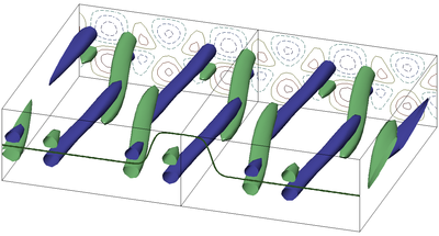
(a)	(b)
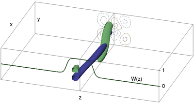
(c)	(d)

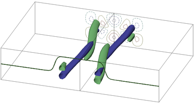
Figure 2: Construction of localized initial guesses by windowing. (a,b) The spatially periodic EQ7 solution of plane Couette flow, in two spatial phases. Three copies of the $\alpha,\gamma=1,2$ periodic solution at $Re=400$ are shown in the $z\in[-3\pi/2,\>3\pi/2]$ subset of the full $L_{x},L_{z}=2\pi,6\pi$ computational domain, with the $z=0$ plane shown bisecting the box to highlight the $z$ symmetries. The solutions in (a) and (b) are related by a quarter-wavelength phase shift in $z$. (c,d) Initial guesses for localized solutions with different symmetry groups, produced by multiplying (a,b) by windowing functions $W(z)$ (heavy line in front planes). Isosurfaces of signed swirling strength at $s=\pm 0.12$ are shown in (green/blue) and contours of streamwise velocity in the back plane at contour levels $u=\pm 0.03\cdot[1\!:\!2\!:\!9]$.

In this section we construct new spanwise localized equilibrium solutions of plane Couette flow by applying windowing and refinement to the spatially periodic EQ7 solution. Figure 2 illustrates how spanwise-localized initial guesses with different symmetry groups are constructed from different spatial phases of the spatially periodic solution. Figure 2(a) shows EQ7 at $Re=400$ with fundamental streamwise and spanwise wavenumbers $\alpha,\gamma=1,2$ (i.e. periodic lengths $\ell_{x}=2\pi/\alpha=2\pi$ and $\ell_{z}=2\pi/\gamma=\pi$). The figure shows three copies of the periodic structure in the $z\in[3\pi/2,\>3\pi/2]$ subset of the full $L_{x},L_{z}=2\pi,6\pi$ computational domain. The spatial phase of EQ7 in figure 2(a) is chosen so that one concentrated vortex structure is centered on the $z=0$ plane. In this phase the solution has symmetry group $\langle\sigma_{xy},\tau_{xz},\tau_{x}\sigma_{z}\rangle$. Each of these symmetries is readily apparent in the figure, keeping in mind that the orientation of swirling with respect to the $x$ axis and thus color of the isosurfaces changes under $\sigma_{xy}$ (rotation about $z$ axis) and $\tau_{x}\sigma_{z}$ ($x$ shift, $z$-reflect symmetry). The windowing function $W(z)$ is plotted as a function of $z$ in the front face of the box. Multiplication of the periodic structure shown in figure 2(a) by the windowing function, followed by projection onto the divergence-free subspace, produces the initial guess shown in figure 2(c). In this case the windowing parameters $a,b=0.3,1$ were chosen to preserve the single concentrated vortex structure centered on the $z=0$ plane and to taper rapidly to nearly zero before the next vortical structure. As discussed in § 2.3, localization in $z$ breaks the $\tau_{xz}$ symmetry of the periodic solution, since it involves $z$ periodicity, leaving a localized initial guess with symmetry group $\langle\sigma_{xy},\tau_{x}\sigma_{z}\rangle$. Any solution in this symmetry group will be an equilibrium, since the $x$ reflection in $\sigma_{xy}$ prevents travelings waves in $x$ and the $z$ reflection in $\tau_{x}\sigma_{z}$ symmetry prevents traveling waves in $z$.

Figure 2(b,d) illustrate construction of a localized initial guess with different symmetries by windowing the periodic solution in a different spanwise phase. Figure 2(b) shows the same periodic EQ7 solution as in figure 2(a), but translated by a quarter-wavelength in $z$. In this phase the periodic NBCW solution has symmetries $\langle\sigma_{xy},\sigma_{z},\tau_{xz}\rangle$, which are again readily apparent in the figure (and which can be derived by conjugating $\langle\sigma_{xy},\tau_{xz},\tau_{x}\sigma_{z}\rangle$ with $\tau_{z}^{1/4}$ and choosing the specified symmetries as generators for the conjugated group). A wider windowing function, with $a=b=1$, preserved a pair of mirror-symmetric concentrated vortical structures in the core region and tapered rapidly to nearly zero before reaching the next vortices, as shown in figure 2(b). The windowing breaks symmetries with factors of $\tau_{xz}$, producing an initial guess for a spanwise-localized solution with symmetry group $\langle\sigma_{xy},\sigma_{z}\rangle$. Again, sign changes in all three coordinates in this symmetry group fix the phase of the velocity field with respect to the origin and rule out traveling waves. Thus, the localized solutions in both choices of $z$ phase will be equilibria, unlike the localized solutions of SGB10, where one choice of phase produces equilibria and the other streamwise-traveling waves.

The localized initial guesses depicted in figure 2(c,d) were then refined to numerically exact equilibrium solutions of plane Couette flow shown in figure 3(a,b), using a Newton-Krylov-hookstep search algorithm. The search algorithm finds equilibria as solutions of the equation ${\bf f}^{T}({\bf u})-{\bf u}=0$, where ${\bf f}^{T}$ is the time-$T$ integration of the discretized Navier-Stokes equations with appropriate boundary conditions. The time integration is performed with a Fourier-Chebyshev-tau scheme in primitive variables (Spalart et al. (1991); Canuto et al. (2006)) and 3rd-order semi-implicit backwards differentiation time stepping (Peyret (2002)). The Fourier-Chebyshev spatial discretization of ${\bf u}({\bf x},t)$ takes the form

$${\bf u}({\bf x})=\sum_{j=-J}^{J}\sum_{k=-K}^{K}\sum_{\ell=0}^{L}\hat{{\bf u}}_{jkl}T_{\ell}(y)e^{2\pi i(jx/L_{x}+kz/Lz)}$$ (4)

Spatial discretization levels are specified by $(J,K,L)$ or by the corresponding $N_{x}\times N_{y}\times N_{z}=(2J\!+\!1)\times L\times(2K\!+\!1)$ physical grid. Nonlinear terms are computed with 3/2-style dealiasing. We set spatial discretization levels so the maximum truncated Fourier and Chebyshev modes are $O(10^{-6})$ and $O(10^{-10})$ respectively. Experience has taught us that coarser spatial discretizations can result in spurious solutions. Symmetries were enforced through the search by projecting ${\bf u}\rightarrow({\bf u}+\sigma{\bf u})/2$ for each of the generators $\sigma$ of the appropriate symmetry group at the intervals $\Delta T=1$ during time integration. The residual of the search equation is $\|{\bf f}^{T}({\bf u})-{\bf u}\|/T$ using the $L^{2}$ norm

$$\|{\bf u}\| =\left[\frac{1}{V}\int_{V}{\bf u}\cdot{\bf u}\,d{\bf x}\right]^{1/2}$$ (5)

where $V$ is the volume of the computational domain. We measure the accuracy of a given solution by increasing spatial resolution by a factor of 3/2 in each direction, decreasing the time step by a factor of 2, and then recomputing the residual. Further details of the implementation of the search algorithm and time integration are given in GHC09, and the code is available for download at www.channelflow.org (Gibson (2013)).

The localized plane Couette solutions depicted in figure 3(a,b) were computed at $Re=400$ in a $2\pi,6\pi$ computational box and a $16\times 65\times 128$ grid, with integration time $T=10$ and time step $dt=0.077$, resulting in a CFL number of about 0.6. The residuals of the windowed initial guesses began at roughly $10^{-3}$ and were reduced to $10^{-15}$ after six or seven iterations of the Newton-Krylov-hookstep algorithm. The $O(10^{-6})$ accuracy of these solutions, measured as discussed above, is the best one could expect given that spectral coefficients were truncated at that level. The tails of the localized solutions drop to $O(10^{-4})$ at the $z=\pm 3\pi$ edge of the computational domain. The computational cost is modest: about one CPU-hour for each solution, running serially on a desktop computer with a 3.3 GHz Intel i7-3960X processor.

2.6 Spanwise localized equilibria of plane Couette flow: roll-streak structure

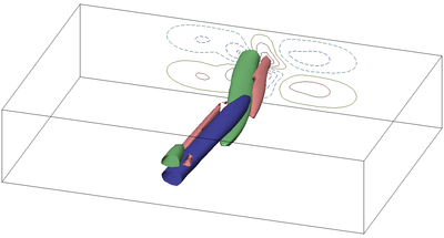
(a)	(b)
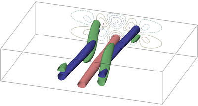
(c)	(d)
(e)	(f)

Figure 3: Spanwise-localized equilibrium solutions of plane Couette flow constructed from windowing the spatially periodic EQ7 equilibrium of Gibson et al. (2009) at $Re=400$, in the $z\in[-3\pi/2,3\pi/2]$ subset of the $L_{x},L_{z}=2\pi,6\pi$ computational domain. (a,b) are localized solutions produced from the initial guesses shown in figure 2(c,d). See text for discussion of (c-f). The plotting conventions are the same as in figure 2, but additionally isosurfaces of streamwise velocity at $u=0.18$ are plotted in red to show the positions of high-speed streaks near the lower wall (symmetric high-speed streaks near the upper wall are not shown).

Figure 3 shows six spanwise-localized equilibrium solutions of plane Couette flow with streamwise wavenumber $\alpha=1$ and $Re=400$. Figure 3(a-d) were obtained by the localization and search methods outlined in § 2.5, (a,b) as described in detail in § 2.5 and (c,d) by increasing the core region of the window to fit three and four copies of the concentrated vortex structures respectively. Solutions (a-d) show that it is possible to obtain localized versions of EQ7 with 1,2,3, and 4 copies of the basic concentrated vortical structure shown in isolation in (a), by choosing appropriate centers of symmetry and width of the core region of the windowing function. We will refer to the solutions (a,b,c,d) as EQ7-1,2,3,4 respectively. Odd-numbered solutions have $\langle\sigma_{xy},\tau_{x}\sigma_{z}\rangle$ symmetry and even-numbered solutions $\langle\sigma_{xy},\sigma_{z}\rangle$. We note that each of the EQ7-1,2,3,4 solutions lies on a distinct solution branch. This is in distinct contrast to the localized versions of the NBCW solutions, for which all solutions with the same symmetry lie on a single solution branch, and additional copies of the fundamental structure are added in a continuous fashion under continuation in Reynolds number, via homoclinic snaking (Schneider et al. (2010)). The localized EQ7 solutions, in contrast, can each be continued in Reynolds number around a single saddle-node bifurcation, and solutions on the opposite branch have distinctly different physical structure. For example, figure 3(e) and (f) show the opposite branches of (b) EQ7-2 and (d) EQ7-4, obtained by continuing these downward in Reynolds, around a saddle-node bifurcation, and back upwards to $Re=400$.

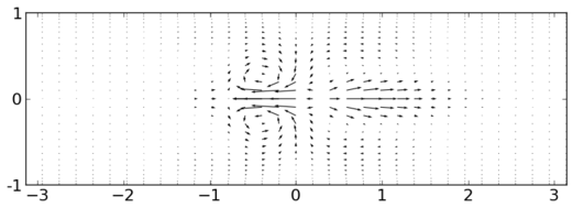
(a)	(f)
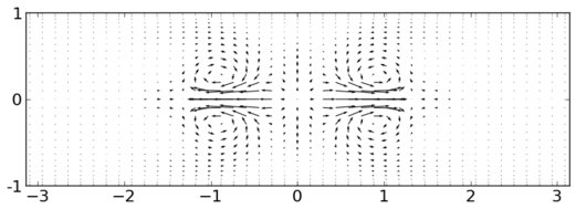
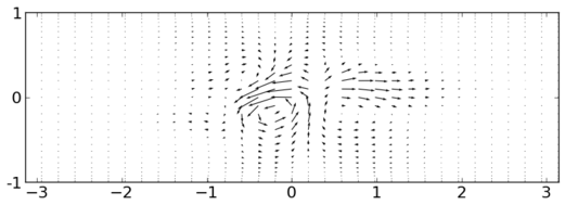
(b)	(g)
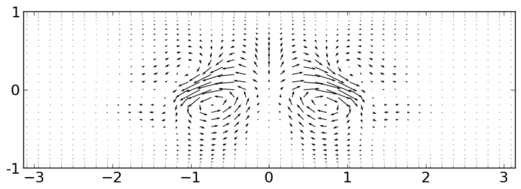
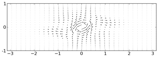
(c)	(h)
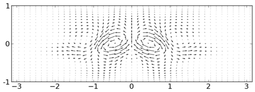
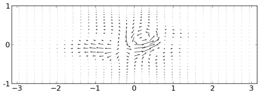
(d)	(i)
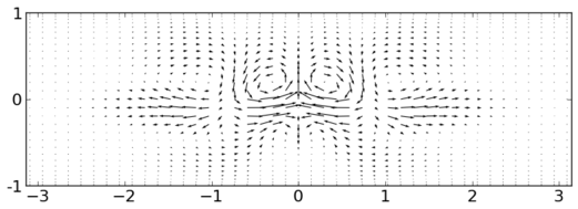
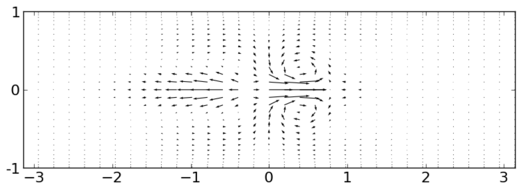
(e)	(j)

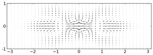
Figure 4: Cross-sections of spanwise-localized equilibrium solutions of plane Couette flow. (a-e) Quiver plots of $[v,w](y,z)$ for EQ7-1 at $x=\{-\pi,-3\pi/4,-\pi/2,-\pi/4,0\}$ with $y$ vertical and $z$ horizontal. (f-j) EQ7-2 at same $x$ values. $\alpha=1$ and $Re=400$ for both. Compare to the same solutions shown with isosurfaces of signed swirling strength in figure 3(a) and (b); the cross-sections here are evenly spaced along the front half of those figures. The $z\in[-\pi,\pi]$ subset of the full $z\in[-3\pi,3\pi]$ computational domain is shown.

The spatial structure of EQ7-1 and EQ7-2 is illustrated in more detail in Figure 4. Figure 4(a-e) show the cross-stream velocity $[v,w](yz)$ for EQ7-1 in five streamwise-normal cross-sections spaced evenly between $x=-\pi$ and $x=0$, which are the front face and the middle of the boxes in figure 3(a,b). The blue isosurface of signed swirling strength in the front half of the box in figure 3(a) appears here as a concentrated counter-clockwise vortex that begins just below and to the left of the origin at $x=-\pi$ in (a), increases in strength and moves upward and to the right in (b-d), and ends above and to the right of the origin at $x=0$ in (e). By the $\tau_{x}\sigma_{z}$ symmetry of EQ7-1, the equivalent quiver plots for $x=0$ through $x=\pi$ would be the $z$-mirror images of (a-e), showing a concentrated clockwise vortex starting below and to the right of the origin and moving upwards and leftwards, and corresponding to the green isosurface of signed swirling strength in the back half of the box in figure 3(a). Likewise, the predominant features of EQ7-2 shown in figure 3(f-j) are two $z$-symmetric counter-rotating vortices that begin near the lower wall at $x=-\pi$ in (f), and rise upwards and closer together in (g-j). Due to EQ7-2’s $\sigma_{xy}$ symmetry, cross-sections from $x=0$ to $\pi$ would appear as the $y$-mirror images of (j-f), with a pair of nearby counter-rotating vortices in the lower half of the $(y,z)$ plane rising and separating, as in the back half of figure 3(b). The clear and distinct concentrations of circulating fluid in figure 4 constitute our main justification for speaking of “regions of concentrated vortical structure” and show that isosurface plots of signed swirling strength are not misleading but rather show precisely where such regions lie.

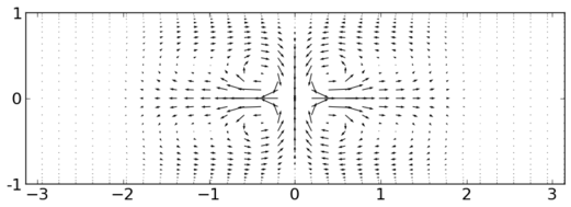
(a)	(c)
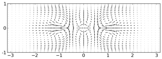
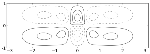
(b)	(d)

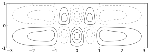
Figure 5: Streamwise-averaged roll-streak structure of spanwise-localized equilibria of plane Couette flow. (a) Quiver plot of $x$-average $[v,w](y,z)$ and (b) contour plot of $x$-average $u(y,z)$ for EQ7-1 with $y$ vertical and $z$ horizontal. (c,d) Same for EQ7-2. Both solutions are shown at $\alpha=1$ and $Re=400$. Contour lines are plotted at levels $u=\pm\{0.03,0.09,0.15\}$, with negative values in dashed lines positive in solid. Quiver plots are autoscaled. The $z\in[-\pi,\pi]$ subset of the full $z\in[-3\pi,3\pi]$ computational domain is shown.

The mean roll-streak structure of EQ7-1 and EQ7-2 is illustrated in Figure 5. The four counter-rotating vortices surrounding the origin in figure 5(a) result from $x$-averaging the counter-clockwise vortex that slopes upwards and rightwards from $x=-\pi$ to $0$ in figure 3(a) and figure 4(a-e) with its clockwise $\tau_{x}\sigma_{z}$-symmetric counterpart that slopes upwards and leftwards from $x=0$ to $\pi$. These four vortices create the pattern of alternating positive and negative streamwise streaks (relative to laminar flow) shown in (b) by advecting high-speed fluid ($u_{\text{tot}}=\pm 1$) from the walls towards the interior in the region near $z=0$, and low-speed fluid ($u_{\text{tot}}\approx 0$) from interior towards the walls for larger $z$. Figure 3(c,d) shows the corresponding mean roll-streak structure for EQ7-2; here the doubling of the basic concentrated vortex structure compared to EQ7-1, apparent in figure 3(b), results in the eight counter-rotating mean vortices shown in (c) and an increased pattern of alternating streamwise streaks shown in (d).

3 Traveling wave solutions of channel flow

In this section we extend the results of § 2 to channel-flow conditions. For the first set of solutions, we use a numerical continuation method similar in spirit to Waleffe’s homotopy of the NBCW solution between plane Couette and “half-Poiseuille” flow with no-slip at the lower wall and free-slip conditions at the upper wall (Waleffe (1998, 2001)). When extended by symmetry to full channel conditions, Waleffe’s continuation produces a traveling-wave solution symmetric about the channel midplane, with two NBCW-like roll-streak structures, each positioned in the high-shear region near either wall, and mirror symmetric ($\sigma_{y}$) to each other across the midplane.

In the present study, we continue the EQ7 solutions from plane Couette to full channel conditions, enforcing no-slip boundary conditions on both walls throughout. The continuation is done in two stages: first with fixed wall speed and increasing pressure gradient, then fixed pressure gradient and decreasing wall speed. As in § 2.1, we decompose the total velocity field into a base flow and a deviation, ${\bf u}_{\text{tot}}({\bf x},t)={\bf u}({\bf x},t)+U(y)\,{\bf e}_{x}$, and the total pressure field into $p_{\text{tot}}=p({\bf x},t)+x\;dP\!/\!dx$, where $dP/dx$ is a parametric constant corresponding to the externally imposed mean pressure gradient. To make the decomposition unique, we specify that the fluctuation pressure $p$ is periodic (so that the spatial mean of ${\bf\nabla}p$ is zero), and that the laminar velocity profile satisfies the no-slip conditions at the walls and balances the imposed mean pressure gradient, $dP\!/\!dx=\nu U^{\prime\prime}$, where $\nu$ is the kinematic viscosity of the fluid. Consequently the base flow is the laminar solution for the given viscosity, mean pressure gradient, and wall speed, and the fluctuation velocity satisfies Dirichlet conditions at the walls. The Navier-Stokes equations again take the form of (1). The Reynolds number $Re=\bar{U}h/\nu$ is based on a velocity scale $\bar{U}$ appropriate to the flow as it transforms from plane Couette to pressure-driven channel conditions, namely, $\bar{U}$ is half the relative wall speed when continuing in pressure gradient and the centerline velocity of the laminar base flow when continuing in wall speed ($\bar{U}=|dP\!/\!dx|\;h^{2}/(2\nu)$). Thus in nondimensional terms the continuation is first in mean pressure gradient $dP/dx$ from 0 to $-2/Re$ with wall speeds fixed at $U(\pm 1)=\pm 1$ (equivalently from $U(y)=y$ to $U(y)=1+y-y^{2}$), and then continuation in wall speed from 1 to 0 with mean pressure gradient held fixed at $P_{x}=-2/Re$ (equivalently from $U(y)=1+y-y^{2}$ to $U(y)=1-y^{2}$). For channel flow conditions $U(y)=1-y^{2}$ and $dP\!/\!dx\neq 0$, eqn. (1) and boundary conditions are invariant under any combination of $x$ and $z$ translations and reflections about the $y\!=\!0$ and $z\!=\!0$ midplanes; thus the symmetry group of channel flow is $\langle\sigma_{y},\sigma_{z},\tau(\Delta x,\Delta z)\rangle$, where $\sigma_{y}:[u,v,w](x,y,z)\rightarrow[u,-v,w](x,-y,z)$.

3.1 Spatially periodic traveling wave solutions of channel flow

(a)

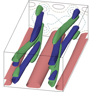
(b)

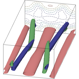
(c)

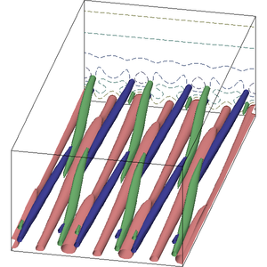
Figure 6: Spatially periodic traveling waves of channel flow with decreasing wall-normal symmetry. (a) TW1, constructed by continuing EQ7 from plane Couette to channel conditions, has symmetry group $\langle\sigma_{y},\sigma_{z},\tau_{xz}\rangle$. Isosurfaces of signed swirling strength are at $s=\pm 0.04$ are shown in green/blue. High-speed streaks near the lower wall are shown by isosurfaces of streamwise velocity at $u=0.02$. High-speed streaks near the upper wall, symmetric to those near the lower wall, are not shown as isosurfaces but they are indicated in the contour plots of streamwise velocity in the back plane. (b) TW2, found from an initial guess judiciously chosen from numerical simulation data, has symmetry group $\langle\sigma_{z},\tau_{xz}\rangle$. Isosurfaces of signed swirling strength at $s=\pm 0.10$ are shown in green/blue, and high-speed streaks near the lower wall are shown by isosurfaces of streamwise velocity at $u=0.03$. There are similar but weaker vortex structures and high-speed streaks near the upper wall, but they do not appear at these levels for the isosurfaces. Both (a) and (b) are shown at $\alpha,\gamma=1,2$ and $Re=2300$. (c) TW3, constructed by continuation in Reynolds number from TW2 and further symmetrization and Newton-Krylov refinement, has $\langle\sigma_{z},\tau_{xz}\rangle$ but periodicity $\alpha,\gamma=1,6$, and is shown at $Re=4000$. Isosurfaces of signed swirling strength are at $s=\pm 0.9$ and $u=0.03$. Each back plane shows contour plot of streamwise velocity at levels $u=\{0.03,-0.03,-0.09,-0.15,...\}$, positive in solid lines and negative in dashed.

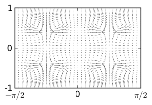
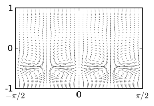
(a)	(b)	(c)
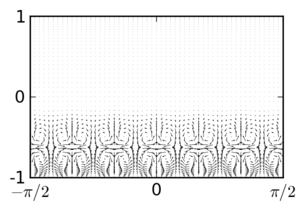
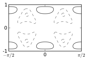
(d)	(e)	(f)

Figure 7: Streamwise-averaged roll-streak structure of spanwise-periodic traveling waves of channel flow. Quiver plots of $x$-average $[v,w](y,z)$ and contour plots of $x$-average $u(y,z)$ for (a,d) TW1, (b,e) TW2, and (c,f) TW3, with the same spatial and Reynolds parameters as in figure 6. Contour lines are shown at levels $u={-0.2,-0.1}$ (dashed) and $u=0.025$ (solid), with an additional negative contour line is shown at $u=-0.3$ in (e). The quiver plots are autoscaled. Axes are $z$ horizontal and $y$ vertical.

TW1: Figure 6(a) and figure 7(a,d) show a spatially periodic traveling-wave solution of channel flow with symmetry $\langle\sigma_{y},\sigma_{z},\tau_{xz}\rangle$ obtained by continuation from plane Couette conditions, as described above. The starting point for continuation was the spatially periodic EQ7 equilibrium of plane Couette flow at $Re=2000$ and $\alpha,\gamma=1,2$; the TW1 channel traveling wave has the same spatial periodicity and is shown at $Re=2300$. Note that TW1 is mirror symmetric about the $y=0$ midplane. The $y$ mirror symmetry is most clearly seen in the streamwise-averaged plots of cross-stream and streamwise velocity in figure 7(a,d). Although $\sigma_{y}$ symmetry is within the symmetry group of channel flow, we did not expect the continuation to produce a solution with this symmetry, since it was neither present in the initial plane Couette solutions nor allowed in the intermediate steps in the continuation from plane Couette to channel conditions. Instead, we expected that the increasing $y$ asymmetry under continuation in pressure gradient would push the vortex structures towards the lower wall, where the shear of the base flow is higher ($|U^{\prime}(-1)|=3$, compared to $|U^{\prime}(1)|=1$, for the base flow $U(y)=1+y-y^{2}$ attained at the end of the pressure continuation), and that this $y$-asymmetry would be maintained during continuation in wall speed down to $U(y)=1-y^{2}$. However, it turned out that weak vortices formed near the upper wall under pressure continuation and grew in strength during wall-speed continuation so that the solution gained $\sigma_{y}$ symmetry when the wall speed reached zero. In terms of the symmetry groups, the starting plane Couette solution had symmetry group $\langle\sigma_{xy},\sigma_{z},\tau_{xz}\rangle$, continuation to nonzero $dP/dx$ broke $\sigma_{xy}$ symmetry, and $\sigma_{y}$ was gained at the final step of wall-speed continuation, resulting in symmetry $\langle\sigma_{y},\sigma_{z},\tau_{xz}\rangle$. The structure of vortices and streaks in TW1 can roughly be described as two copies of EQ7 stacked on top of each other, with the upper copy either phase-shifted by half a wavelength in $x$ or having $[v,w]$ reversed in sign via mirror symmetry in $y$. This is apparent from comparison of TW1 in figure 6(a) to EQ7 in figure 1(b) and EQ7-1 in 3(b).

TW2: Figure 6(b) and figure 7(b,e) show a spatially periodic traveling-wave solution of channel flow with asymmetry in $y$ and symmetry $\langle\sigma_{z},\tau_{xz}\rangle$, obtained from an initial guess from turbulent simulation data (Viswanath (2007); Gibson et al. (2009)). Specifically, we $z$-mirror-symmetrized an arbitrary turbulent velocity field of channel flow at $Re=3750$ in a $2\pi,1\pi$ box by applying ${\bf u}\rightarrow 1/2\;(1+\sigma_{z}){\bf u}$ and then quenched the turbulent field by lowering the Reynolds number and continuing time integration with the bulk velocity fixed at 2/3 and the $\sigma_{z}$ symmetry enforced by projection at regular intervals. After some experimentation, we found that after quenching to $Re=2650$, the fine-scale structure of the velocity field and the spatial-mean wall shear decreased quickly, the latter reaching a local minimum after about 50 time units and growing slowly again for another 50 time units before resuming a high level of wall shear with rapid fluctuations. The smoothness and length of this minimum suggested a close pass to a hyperbolic edge state. Using a velocity field from this minimum as an initial guess for a Newton-Krylov search produced a numerically exact spatially periodic, wall-localized traveling wave solution of channel flow with $\langle\sigma_{z},\tau_{xz}\rangle$ symmetry.

The $y$ asymmetry of TW2 is exaggerated in figure 6(b) by the binary character of isosurface plots. In fact at $Re=2300$ TW2 has weaker vortex structures near the upper wall with swirling strength comparable to those of TW1, and weaker streaks there as well. Both the vortices and streaks near the upper wall are visible in the streamwise-average plots of TW2 in figure 7(b,e). Note also that the swirling strength isosurfaces of TW2 in figure 6(b) are at $s=\pm 0.10$, over twice the magnitude of those for TW1 in figure 6(a) at $s=\pm 0.4$. Compared to the four layers of counter-rotating mean vortices stacked symmetrically about $y=0$ in TW1 (see Figure 7(a,d)), TW2 has two layers of counter-rotating mean vortices below $y=0$ and a single layer of vortices above $y=0$, and these vortices have the same orientation as the vortices below them. And though it is not clear from the autoscaled quiver plots, the mean vortices of TW2 near the lower wall are about three times the magnitude of those of TW1, as measured by magnitudes of the $[v,w]$ velocities, and the mean vortices of TW2 above $y=0$ are of comparable magnitude to those of TW1. However, the $y$-asymmetry of TW2 increases as the Reynolds number is increased (see TW3) and as $z$-periodicity is relaxed (see TW2-1 and TW2-2).

TW3: Figure 6(c) and figure 7(c,f) show a wall-localized, spanwise and streamwise periodic traveling wave of channelflow with symmetry $\langle\sigma_{z},\tau_{xz}\rangle$, discovered through continuation of TW2 in Reynolds number. The fundamental $z$ wavenumber of TW2 is $\gamma=2$, but as as $Re$ increased towards $4000$, the structure at this wavenumber weakened and structure at $\gamma=6$ grew, while the structure away from the lower wall weakened substantially until it became nearly laminar. TW3 was computed by zeroing all modes in TW2 at $Re=4000$ with $\gamma<6$ and refining this initial guess to an exact traveling wave with Newton-Krylov-hookstep search. The resulting TW3 solution has periodicity $\alpha,\gamma=1,6$ and symmetry $\langle\sigma_{z},\tau_{xz}\rangle$, where $\tau_{xz}$ is understood as involving a half-cell shift in $z$ with respect to the smaller $\ell_{z}=\pi/3$ periodic length. Its most notable property is its very strong localization in the wall-normal direction, as evidenced by figure 7(c,f).

3.2 Spanwise localized traveling wave solutions of channel flow

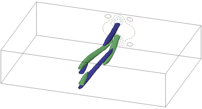
(a)	(b)
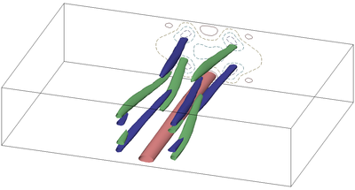
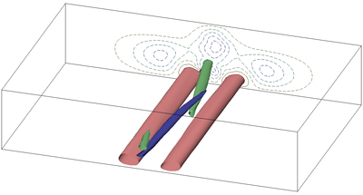
(c)	(d)

Figure 8: Spanwise-localized traveling wave solutions of channel flow. (a) TW1-1, (b) TW1-2, (c) TW2-1, and (d) TW2-2. (a,b) TW1-1 and TW1-2 are $\langle\sigma_{y},\tau_{x}\sigma_{z}\rangle$ and $\langle\sigma_{y},\sigma_{z}\rangle$ symmetric traveling waves obtained by localizing TW1 in two different $z$ phases. (c,d) TW2-1 and TW2-2 are $\tau_{x}\sigma_{z}$ and $\sigma_{z}$ symmetric traveling waves obtained by localizing TW2 in two different $z$ phases. Plotting conventions are the same as in figure 6, but with isosurfaces of signed swirling strength and streamwise velocity at (a,b) $s=\pm 0.05$, $u=0.05$, and (c,d) $s=\pm 0.09$, $u=0.08$. Contour lines of streamwise velocity are shown in the back $y,z$ plane at levels $u=0.03$ (solid lines) and (a,b) $u=\{-0.03,-0.09,-0.15\}$, (c,d) $u=\{-0.03,-0.09,-0.15,-0.21,-0.30\}$ (dashed). In (b) a high-speed streak near the upper wall, symmetric to that near the lower wall, is suppressed to avoid visual clutter. By contrast, (c,d) show true asymmetry in high-speed speed streaks: (c) has high-speed streaks near the lower wall only, and in (d) the streaks near the upper wall are substantially weaker, below the given isosurface levels. Solutions are shown at $Re=2300$ in $z\in[-3\pi/2,\>3\pi/2]$ subsets of their full $L_{x},L_{z}=2\pi,6\pi$ computational domains.

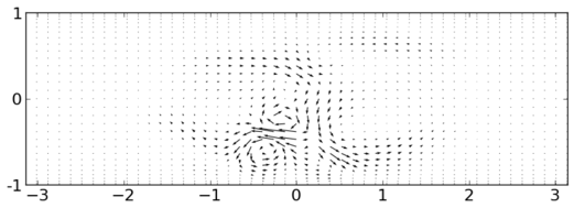
(a)	(f)
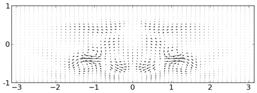
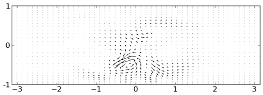
(b)	(g)
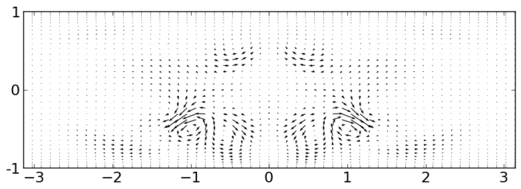
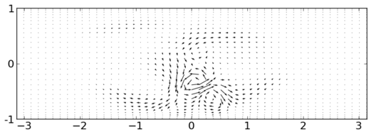
(c)	(h)
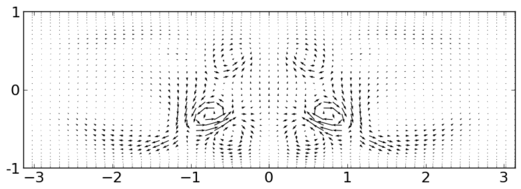
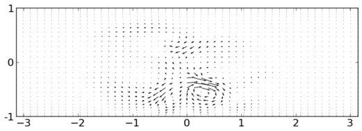
(d)	(i)
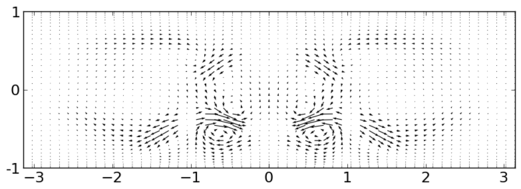
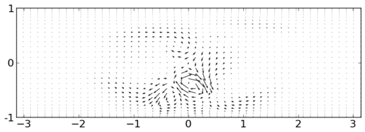
(e)	(j)

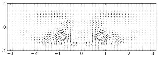
Figure 9: Cross-sections of spanwise-localized, near-wall traveling waves of channel flow. (a)-(e) Quiver plots of $[v,w](y,z)$ for TW2-1 at $x=\{-\pi,-0.6\pi,-0.2\pi,0.2\pi,0.6\pi\}$, (f)-(j) same for TW2-2, with $y$ vertical and $z$ horizontal. Both solutions are at $\alpha=1$ and $Re=2300$. The $z\in[-\pi,\pi]$ subset of the full $z\in[-3\pi,3\pi]$ computational domain is shown.

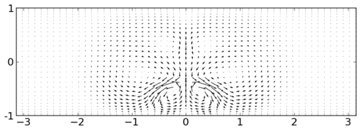
(a)	(c)
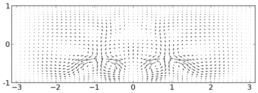
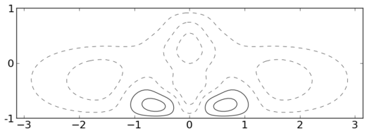
(b)	(d)

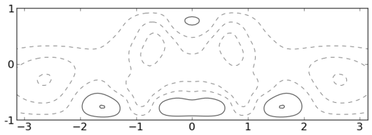
Figure 10: Streamwise-averaged roll-streak structure of spanwise-localized traveling waves of channel flow. (a) Quiver plot of $x$-average $[v,w]$ and (b) contour plot of $x$-average $u(y,z)$ for TW2-1. (c,d) Same for TW2-2. $\alpha=1,Re=400$ for both solutions. Contour lines are plotted at levels $u=\{-0.25,-0.15,-0.05,0.05,0.15\}$, with negative values in dashed lines and positive in solid. Quiver plots are autoscaled. The $z\in[-\pi,\pi]$ subset of the full $[-3\pi,3\pi]$ computational domain is shown.

In this section we construct spanwise-localized traveling wave solutions of channel flow by windowing the spanwise-periodic travelings waves of § 3.1 TW1 and TW2 in different spatial phases. The resulting solutions are illustrated in figure 8, figure 9, and figure 10.

TW1-1, shown in figure 8(a), was formed by phase-shifting TW1 in $z$ by $\pi/4$ to give it symmetry group $\langle\sigma_{y},\sigma_{z}\tau_{x},\tau_{xz}\rangle$, extending this periodic solution from a $2\pi,1\pi$ to a $2\pi,6\pi$ box, windowing the extended periodic solution, and then applying Newton-Krylov-hookstep refinement to the windowed initial guess, producing a spanwise-localized traveling wave with $\langle\sigma_{y},\sigma_{z}\tau_{x},\rangle$ symmetry. The windowing parameters $a,b=0.5,0.4$ were chosen to isolate the central vortex structures in swirling-strength plots. It did not take a great deal of effort to find windowing parameters that gave a successful initial guess; we merely adjusted $a$ and $b$ by tenths until swirling-strength plots of the initial guess appeared similar to the resultant solution in figure 8(a). The initial guess for the wave speed was set to the wave speed of the underlying periodic solution TW1, and the pressure gradient was held fixed at $dP/dx=-2/Re$ where $Re=2000$. The Newton-Krylov-hookstep search converged to machine precision in six steps, consuming about half an hour of single-core CPU time on the machine described in § 2.5, for a $20\!\times\!81\!\times\!256$ discretization of the $2\pi,6\pi$ computational domain. The computed solution turned out to be smoother in $x$ and $z$ than the periodic solution on which it was based, enough that $10^{-6}\!\times\!10^{-10}\!\times\!10^{-6}$ truncation levels were retained on a reduced grid of $12\!\times\!81\!\times\!192$. Similarly TW1-2 figure 8(b) was found by refining an initial guess formed from windowing TW1 in in its $z$-phase with $\langle\sigma_{y},\sigma_{z},\tau_{xz}\rangle$ symmetry and with windowing parameters $a,b=1.2,0.4$, resulting in a traveling wave solution with $\langle\sigma_{y},\sigma_{z}\rangle$ symmetry.

TW2-1 and TW2-2, shown in figure 8(c,d), are likely the most interesting solutions presented in this paper, as they represent traveling wave solutions that are spanwise localized and strongly concentrated near a single wall, and as such are the solutions most likely to be relevant to the lambda-vortex coherent structures that occur near the walls of shear flows (Saiki et al. (1993)). TW2-1 was formed by windowing TW2 in its $z$-phase with symmetry $\langle\tau_{x}\sigma_{z},\tau_{xz}\rangle$ and windowing parameters $a,b=0.6,0.4$ to get an initial guess with $\tau_{x}\sigma_{z}$ symmetry, and refining that with Newton-Krylov-hookstep. We were unable to form TW2-2 by the phase-shifting, windowing, and refining procedure employed for other localized solutions. Instead TW2-2 was formed by shifting TW2-1 leftwards in $z$ until its right-hand high-speed streak was centered on $z=0$, extending the shifted field on $z\leq 0$ onto $z\geq 0$ by $z$-mirror symmetry, and then refining this initial guess with Newton-Krylov-hookstep. We note that TW2-1 and TW2-2 required finer grids to resolve the stronger vortex structure adequately compared to TW1-1 and TW1-2. Larger computational domains were also necessary, due to the increased width of the streamwise velocity deficit (visible as contour lines in the back plane of figure 8). The computations of TW2-1 and TW2-2 from initial guess to took about seven CPU-hours each.

Each of the traveling wave solutions depicted in figure 8 is formed from variations of very similar basic structure, which mostly clearly seen in isolation in TW2-1 in figure 8(c). Near the lower wall there is an $x$-periodic chain of concentrated vortices, alternating in sign of circulation (clockwise/counter-clockwise), and nearly aligned with the $x$-axis but tilting slightly in the wall-normal and spanwise directions, as shown in figure 9(a-e). The tilting of the chain of alternating vortices results in a nonuniform $x$-average in the cross-stream flow, specifically, a pair of counter-rotating mean vortices near the wall, figure 10(a). The mean vortices draw low-speed fluid upwards between them and high-speed fluid downward on either side, producing the mean high-speed streaks on either side of the mean vortex pair, depicted by solid contour lines in figure 10(b). The streamwise momentum exchanged induced by the near-wall mean vortices has a net negative effect: the region of mean streamwise flow slower than laminar indicated by negative (dashed) contour lines in figure 10(b) is larger in both $y,z$ area and magnitude than the high-speed streaks that outpace laminar flow, indicated by solid contour lines. Thus the net effect of the roll-streak structure is a decrease of bulk flow relative to laminar for a fixed pressure gradient. TW2-2 roughly consists of two copies of TW2-1’s basic structure, repeated with mirror-symmetry about the $z=0$ plane. This is evident from comparison of TW2-1 and TW2-2 in figure 8(c) and (d), figure 9(a-e) and (f-g), and figure 10(a,b) and (c,d). TW1-1 and TW1-2 have similar structure to TW2-1 and TW2-0, but with mirror symmetry in $y$ and weaker magnitudes of vorticity (by roughly a factor of two) and net velocity deficit relative to laminar (by a factor of four or more).

The cross-stream quiver plots of these exact wall-bounded traveling waves, figures 8 and 10 bear intriguing resemblances to the cross-sections of near-wall lambda vortices of developing channel flow shown in Saiki et al. (1993) figures 10 and 11. For example, the streamwise mean $v,w$ flow of TW2-1 in figure 10 is strikingly like the temporal-mean $v,w$ of the K-type-generated lambda vortex shown in Saiki et al. (1993) figure 10(b). The $\Lambda$-structure shown in Saiki et al. (1993) figure 2(b) is evident in TW2-2 in figure 8(d). Of course the traveling waves in this paper are exact solutions of different flow conditions than the spatially-developing channel flow of Saiki et al. (1993), so some translation of the flow conditions is required to make more precise comparisons. We intend to pursue this in future research.

	symmetry	$\alpha,\gamma$	$Re$	$c$	$L_{x},L_{z}$	grid	accur.	tails
TW1	$\langle\sigma_{y},\sigma_{z},\tau_{xz}\rangle$	$1,2$	2300	0.673	$2\pi,\pi$	$16\!\times\!81\!\times\!32$	$10^{-7}$	-
TW1-1	$\langle\sigma_{y},\tau_{x}\sigma_{z}\rangle$	$1,-$	2300	0.674	$2\pi,6\pi$	$12\!\times\!81\!\times\!192$	$10^{-6}$	$10^{-5}$
TW1-2	$\langle\sigma_{y},\sigma_{z}\rangle$	$1,-$	2300	0.674	$2\pi,6\pi$	$12\!\times\!81\!\times\!192$	$10^{-6}$	$10^{-5}$
TW2	$\langle\sigma_{z},\tau_{xz}\rangle$	$1,2$	2300	0.564	$2\pi,\pi$	$24\!\times\!97\!\times\!48$	$10^{-6}$	-
TW2-1	$~{}\tau_{x}\sigma_{z}$	$1,-$	2300	0.661	$2\pi,6\pi$	$16\!\times\!97\!\times\!216$	$10^{-6}$	$10^{-5}$
TW2-2	$~{}\sigma_{z}$	$1,-$	2300	0.648	$2\pi,6\pi$	$16\!\times\!97\!\times\!216$	$10^{-6}$	$10^{-5}$
TW3	$\langle\sigma_{z},\tau_{xz}\rangle$	$1,6$	4000	0.475	$2\pi,\pi/6$	$24\!\times\!109\!\times\!24$	$10^{-6}$	-

Table 1: Characteristics of traveling-wave solutions of channel flow.

Table 1 summarizes physical characteristics and discretization properties of the computed traveling-wave solutions of channel flow. Wave speed $c$ is in nondimensionalized units where the centerline velocity of laminar flow is $\bar{U}=1$. $L_{x},L_{z}$ are the size of the computational domain. Accuracy is measured as $\|{\bf f}^{T}({\bf u}))-\tau{\bf u}\|/T$ for $T=10$, where ${\bf f}^{T}$ is the time-$T$ forward time integration of the Navier-Stokes as performed by direct numerical simulation, and where $\tau=\tau(cT,0)$ is the $x$-translation resulting from the computed wave speed $c$ over time $T$. The magnitude of the tails is given as the maximum of $|u|,|v|$ and $|w|$ over $x,y$ at $z=\pm L_{z}/2$, the edge of the spanwise-extended periodic box.

4 Discussion

4.1 Exponential decay of tails

The spanwise localized solutions presented in this paper display a three-part structure: a core region that closely resembles a periodic solution, a transition region, and weak tails that decay to laminar flow. In this section we show that the tails of spanwise-localized streamwise-periodic equilibria are dominated by a mode that decays exponentially at $e^{-\alpha|z|}$, where $\alpha$ is the fundamental streamwise wavenumber, and that the structure of the tails depends on flow parameters $\alpha,Re$, the laminar flow profile $U(y)$, and the wavespeed $c$, but not on the details of the solution’s core region.

As the tails of a spanwise-localized equilibrium or traveling wave approach laminar flow, the perturbation velocity ${\bf u}$ approaches zero, so we expect ${\bf u}$ to approximately satisfy the linearized form of (1) in which ${\bf u}\cdot{\bf\nabla}{\bf u}$ is set to zero,

$$\frac{\partial{\bf u}}{\partial t}+U\frac{\partial{\bf u}}{\partial x}+v\>U^{\prime}\>{\bf e}_{x}=-\nabla p+\frac{1}{Re}\nabla^{2}{\bf u},\quad\nabla\cdot{\bf u}=0.$$ (6)

We look for normal-mode solutions of the form

$${\bf u}_{j,\gamma}({\bf x})=\tilde{{\bf u}}_{j,{\gamma}}(y)\>e^{i(j\alpha(x-ct)+\gamma z)},\quad p_{j,\gamma}({\bf x})=\tilde{p}_{j,{\gamma}}(y)\>e^{i(j\alpha(x-ct)+\gamma z)}$$ (7)

where $\alpha$ is real and $\gamma=\gamma_{r}+i\gamma_{i}$ has $\gamma_{i}>0$ for tails that decay exponentially as $z\rightarrow\infty$. The slowest decaying normal mode solution, with the smallest positive $\gamma_{i}$, will dominate the tails as $z\rightarrow\infty$. For the remainder of this section we drop the $j,\gamma$ subscripts. To eliminate pressure we convert to velocity-vorticity form by taking the $y$-components of the curl and the curl of the curl of (6)

$$\left(\frac{\partial}{\partial t}+U\frac{\partial}{\partial x}\right)\eta+U^{\prime}v_{z} =\frac{1}{Re}\nabla^{2}\eta,$$

$$\left(\frac{\partial}{\partial t}+U\frac{\partial}{\partial x}\right)\nabla^{2}v-U^{\prime\prime}v_{x} =\frac{1}{Re}\nabla^{4}v,$$ (8)

where $\eta=u_{z}-w_{x}$ is the wall-normal vorticity. Boundary conditions are $\eta(x,\pm 1,z)=0$ and $v(x,\pm 1,z)=v^{\prime}(x,\pm 1,z)=0$.

Eqn. 8 and boundary conditions permit a number of types of solution. Where symmetries allow, the solution that dominates behavior in the tails of localized plane Couette equilibria and traveling waves turns out to be the trivial solution $v=\eta=0$. This solution in conjunction with the divergence-free condition and the ansatz (7) requires that $\tilde{u}_{xx}=-\tilde{u}_{zz}$ and $\tilde{w}_{xx}=-\tilde{w}_{zz}$, which is satisfied by $\gamma=\pm ij\alpha$ and $\tilde{w}=\pm ij\tilde{u}$, the different signs governing exponential decay in the different limits $z\rightarrow\pm\infty$. The $j=1$ mode with $\gamma=\pm i\alpha$ and $\tilde{w}=\pm i\tilde{u}$ thus gives the slowest exponential decay rate ($j=0$ is ruled out since it does not decay and thus cannot be part of a $z$-localized solution). The $y$ component of (6) gives that $\partial\tilde{p}/\partial y=0$ so that $\tilde{p}(y)=\tilde{p}$ is a complex constant whose magnitude and phase are set by the pressure conditions at the edge of the transition region at some fixed value of $z$. The $x$ component of (6) gives

$$\tilde{u}^{\prime\prime}-i\alpha Re(U-c)\tilde{u}=i\alpha Re\;\tilde{p}.$$ (9)

The boundary conditions $\tilde{u}(\pm 1)=0$ set the homogeneous solution to zero, so that $\tilde{u}$ and thus $\tilde{w}$ are determined by the fixed value of $\tilde{p}$, the base flow profile $U(y)$, and the parameters $\alpha$, $c$ and $Re$. They are independent of the structure of the core-region solution (except for differences of $x$ phase between the $\pm z$ tails resulting from the symmetries of the solution). Thus the $v=\eta=0$ solution to the linearized Navier-Stokes equations contributes to the tails an exponentially decaying mode of form $[\tilde{u}(y),\>0,\>i\tilde{u}(y)]e^{i\alpha(x-ct)-\alpha z}$ as $z\rightarrow\infty$.

(a)

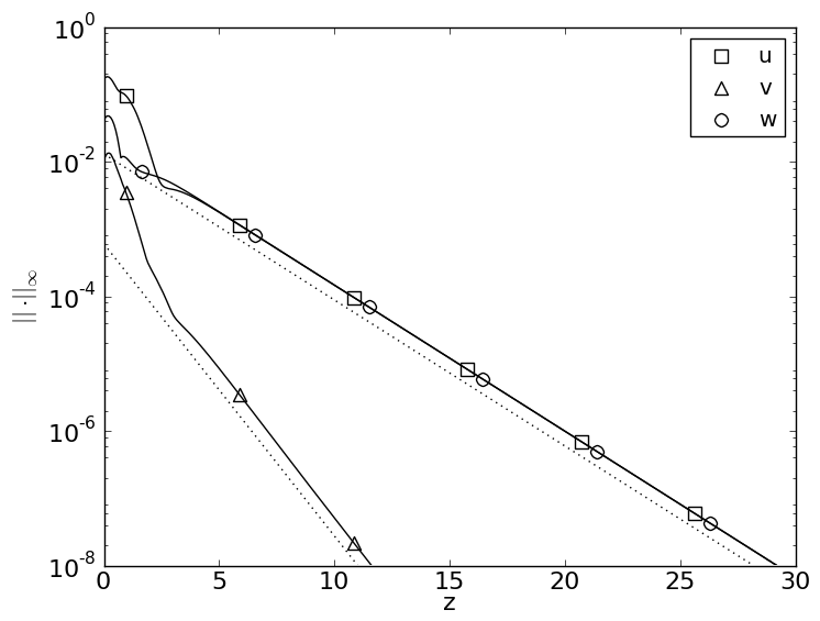
(b)

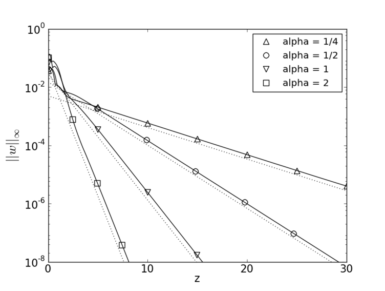
Figure 11: Exponential decay in the tails of spanwise localized plane Couette equilibria. (a) Componentwise decay rates for EQ7-1 at $\alpha=1/2$, $Re=600$: $u,v,w$ (solid lines) scale as $e^{-\alpha z},e^{-2\alpha z},e^{-\alpha z}$ (dotted lines). (b) Decay of $\|w\|_{\infty}$ for EQ7-1 (solid lines) compared to $e^{-\alpha z}$ (dotted lines) at $Re=600$ and several values of $\alpha$.

Figure 11 confirms that over a wide range of $\alpha$, the tails of EQ7-1 are dominated by $u,w$ components that decay as $e^{-\alpha z}$. Figure 11(a) shows the inf-norm of $u,v$ and $w$ as a function of $z$ for EQ7-1 at $\alpha=1$. In this context $\|u\|_{\infty}(z)$ is the maximum of $|u(x,y,z)|$ over $x,y$ as a function of $z$. As argued above, the magnitudes of the $u$ and $w$ components are equal in the tails and scale as $e^{-\alpha z}$. The higher-order $e^{-2\alpha z}$ scaling for $v$ results from the quadratic nonlinear term in $u_{1,\gamma},w_{1,\gamma}$ that has been suppressed on the right-hand side of (6) for the $v_{0,\gamma}$ equation in for $j=0$. For figure 11(b), we continued EQ7-1 parametrically in $\alpha$ and observed that the $e^{-\alpha z}$ scaling holds over the explored range of $1/4\leq\alpha\leq 2$. For further confirmation of the dominance of $v=\eta=0$ modes, figure 12(a) compares an $x,y$ slice of streamwise velocity $u(x,y,z)$ from EQ7-1 at a fixed $z$ to (b) the same as computed from (9).

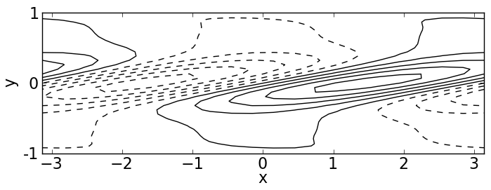
(a) (b)

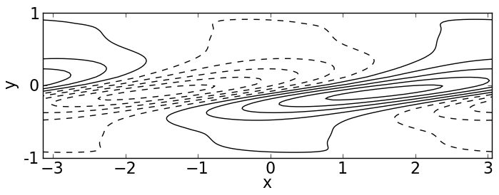
(c)

Figure 12: (a,b) Asymptotic form of the tails of spanwise-localized equilibria of plane Couette flow. Contours of streamwise velocity $u(x,y)$ at fixed $z$: (a) a slice of EQ7-1 for $\alpha=1$ and $Re=400$, at $z=11$, where $||u||_{\infty}\approx 10^{-6}$, and (b) the asymptotic $v=\eta=0$ normal mode solution. Contours are plotted at $\pm[0.15,0.45,0.75]$ times the maximum of $u$, with negative values in dashed lines. (c) Exponential decay rate for three types of normal modes in the tails of plane Couette equilibria at $Re=400$. The minimal $\gamma_{i}$ as a function of $\alpha$ is plotted for ($\square$) $v=\eta=0$ solutions, ($\circ$) solutions of (10) with $\tilde{v}(y)=0$, and ($\triangleright$) solutions of (11).

The linearized equations for the tails have solutions other than $v=\eta=0$; to show these decay more rapidly than the $v=\eta=0$ modes (for plane Couette flow), we reduce eqn. 8 to the eigenvalue equations

$$i\alpha(U-c)\tilde{\eta}+i\gamma U^{\prime}\tilde{v} =\frac{1}{Re}(\tilde{\eta}^{\prime\prime}-(\alpha^{2}+\gamma^{2})\tilde{\eta}),$$ (10)

$$i\alpha(U-c)(\tilde{v}^{\prime\prime}-(\alpha^{2}+\gamma^{2})\tilde{v})-i\alpha U^{\prime\prime}\tilde{v} =\frac{1}{Re}(\tilde{v}^{\prime\prime\prime\prime}-2(\alpha^{2}+\gamma^{2})\tilde{v}^{\prime\prime}+(\alpha^{2}+\gamma^{2})^{2}\tilde{v}).$$ (11)

The latter is the time-independent form of the familiar Orr-Sommerfeld equation for three-dimensional disturbances. Equation (11) is independent of $\tilde{\eta}$ and the eigenvalues $\gamma$ can be found numerically for given $\alpha$, $c$, $Re$, and $U(y)$. The $i\gamma U^{\prime}\tilde{v}$ coupling term in (10) acts as a nonhomogeneous forcing, requiring particular solutions for $\tilde{\eta}(y)$ to match the eigenmodes of (11). Eigenvalues distinct from those found for (11) can be found by solving (10) with $\tilde{v}(y)=0$. Figure 12(c) shows the minimal $\gamma_{i}$ allowed by these two equations as a function of $\alpha$ for plane Couette equilibria at $Re=400$. Note that $v=\eta=0$ modes have the smallest $\gamma_{i}$ for $\alpha$ in the range shown ($\alpha<2$); thus these modes dominate the behavior of the tails in all solutions with streamwise wavelength greater than $\pi$. It should be noted, however, that streamwise constant ($\alpha=0$) modes can exist in domains of any length $L_{x}$, and thus might play a dominant role in short (large $\alpha$) domains if the symmetries permit them.

4.2 Asymptotic scaling of streamwise Fourier harmonics

In this section we provide a numerical account of the large-Reynolds behavior of the periodic and localized solutions developed in previous sections. In particular we measure the scaling of various streamwise Fourier components of the solutions with $Re$, and we show the development of critical layers at large $Re$. These features are key to the asymptotic analysis of NBCW suggested by Wang et al. (2007) and developed into a complete theory by Hall & Sherwin (2010). The main results are as follows. The streamwise Fourier components of EQ7 and solutions related to it, localized and in channel conditions, obey scaling laws similar to those of NBCW, albeit with different exponents and substantially different magnitudes, suggesting that Hall & Sherwin (2010)’s asymptotic analysis could be carried over to the new solutions. EQ8 and the $y$-asymmetric channel flow solutions, in contrast, do not fit the asymptotic scaling framework so cleanly. All solutions appear to have well-defined critical layers, however, and the critical layer is particularly simple for EQ7 and its localized counterparts.

As suggested by Wang et al. (2007) and developed into a complete theory by Hall & Sherwin (2010), a reduced PDE system can be developed for the spatially periodic NBCW solution from an asymptotic analysis of its streamwise Fourier modes and the critical layer that develops at large Reynolds numbers. Wang et al. (2007) showed numerically that NBCW has a simplified, quasi-2D structure in the limit of large Reynolds numbers, with a balance between an $O(1)$ streamwise-constant streaks, $O(Re^{-1})$ streamwise-constant rolls, and an $O(Re^{-0.9})$ mode in the first (fundamental) streamwise Fourier harmonic, which concentrates in a critical layer of thickness $O(Re^{-1/3})$. Hall & Sherwin (2010) in turn developed an asymptotic theory for NBCW based on vortex-wave interaction that provides insight to the physics of how these components of NBCW balance, predicts their scaling exponents, and which reduces the computation of the solution from a 3D Navier-Stokes problem at large-$Re$ to a 2D PDE at $Re=1$ coupled with a linear wave evolution equation. Specifically, the interactions of very small fundamental-mode streamwise waves within the critical layer generate nonzero mean stresses that cause jumps in the pressure and the normal derivative of roll velocity across the critical layer. The jump in roll shear drives the mean rolls, which in turn drive the mean streaks. Hall & Sherwin (2010) show that these effects balance to leading order in $Re^{-1}$, and that the asymptotic theory also reduces computation of the 3D steady state at high Reynolds number to a simpler 2D calculation at unit Reynolds number coupled with a linear wave evolution equation.

This reduced quasi-2D PDE model of Hall & Sherwin (2010) is of particular interest to us since a theoretical analysis of spanwise localization in solutions of Navier-Stokes should be easier to develop in the context of a reduced model. There is strong numerical evidence that a theory of localization in solutions of Navier-Stokes might be developed. Schneider et al. (2009) noted a remarkable resemblance between the $x,y$-averaged energy of the localized NBCW solutions and localized solutions of the 1d Swift-Hohenberg equation found by Burke & Knobloch (2007). The similarity was made more remarkable by Schneider et al. (2010)’s demonstration that the localized NBCW solutions undergo homoclinic snaking under continuation in Reynolds number, just as the localized Swift-Hohenberg solutions do under continuations in their bifurcation parameter. For Swift-Hohenberg, homoclinic snaking of localized solutions is quite well understood theoretically via “spatial dynamics” (Burke & Knobloch (2007)). Time independence reduces the 4th-order Swift-Hohenberg PDE for $u(x,t)$ to 4th-order ordinary differential equation (ODE) on $u(x)$, which can then considered as a 4-dimensional dynamical system where $x$ plays the role of time. In this view, spatially periodic solutions correspond to periodic orbits of the spatial dynamics, and spatially localized solutions correspond to homoclinic orbits that start at the origin $u=0$ at $t\rightarrow-\infty$, grow away from it along unstable direction, wander at finite amplitude for some time, and then reapproach $u=0$ at $t\rightarrow\infty$ along a stable direction. Localized solutions display approximately periodic form in their core regions when the finite-amplitude excursion away from $u=0$ makes a number of circuits in the neighborhood of an unstable periodic orbit of the spatial dynamics. Thus the close correspendence between localized Navier-Stokes solutions and localized Swift-Hohenberg solutions points to the possibility of a theoretical explanation of localization in invariant solutions of Navier-Stokes. It also points to the importance of a reduced PDE system describing the localized solutions, ideally to a 1d system in the spanwise coordinate, to which the idea of spatial dynamics might be applied. We report on the scaling of streamwise Fourier components and the development of a critical layer in the plane Couette and channel solution because they are essential ingredients for developing such a reduced-order PDE model.

The perturbation velocity field of equilibrium and traveling wave solutions can be expressed as a sum of streamwise ($x$) Fourier modes in the form

$${\bf u}({\bf x},t)=\sum_{j}\hat{{\bf u}}_{j}(y,z)e^{ij\theta}$$ (12)

where $\theta=\alpha(x-ct)$ and where $\hat{{\bf u}}_{-j}(y,z)=\hat{{\bf u}}_{j}^{*}(y,z)$ so that ${\bf u}$ is real-valued. The streamwise constant mode $\hat{{\bf u}}_{0}$ can be decomposed into streamwise streaks $\hat{u}_{0}(y,z)$ and cross-stream rolls $[0,\hat{v}_{0},\hat{w}_{0}](y,z)$. Recall that ${\bf u}$ is the deviation from laminar flow $U(y){\bf e}_{x}$, with ${\bf u}_{\text{tot}}={\bf u}+U(y){\bf e}_{x}$ and $\hat{u}_{\text{tot},0}=\hat{u}_{0}+U(y)$, so that the streaks are defined relative to laminar flow. Wang et al. (2007) define streaks relative to the $z$-averaged mean flow, but we do not, since $z$-averaging is inappropriate for spanwise-localized solutions. Hall & Sherwin (2010) refer to the first (fundamental) harmonic $\hat{{\bf u}}_{1}(y,z)$ or $\hat{{\bf u}}_{1}(y,z)\exp(i\alpha(x-ct))+\text{c.c.}$ as the wave mode.

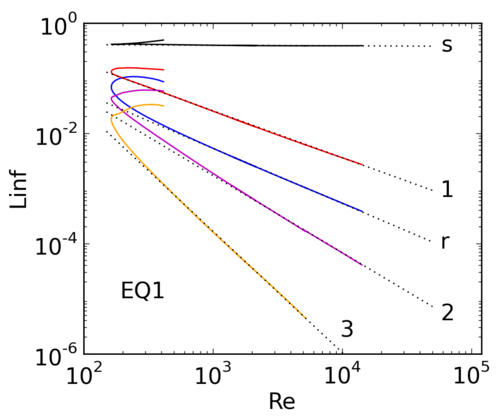
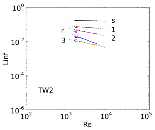
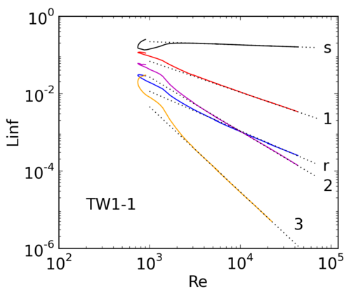
(a)	(b) (c)
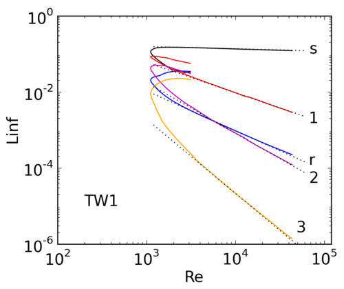
(d)	(e) (f)
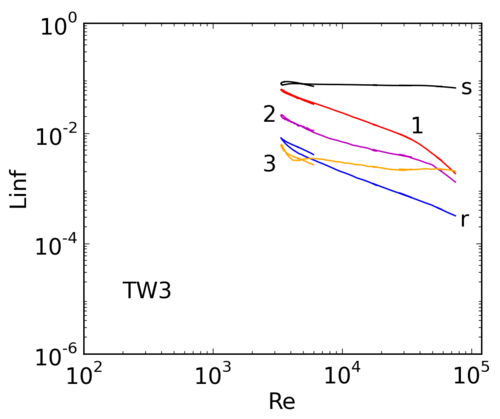
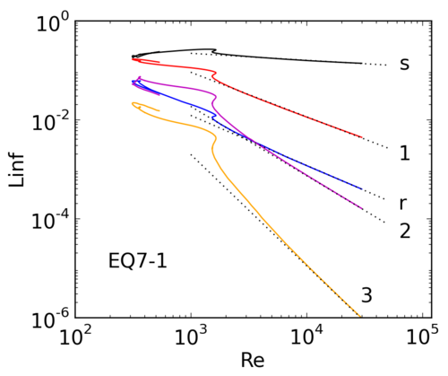
(g)	(h) (i)

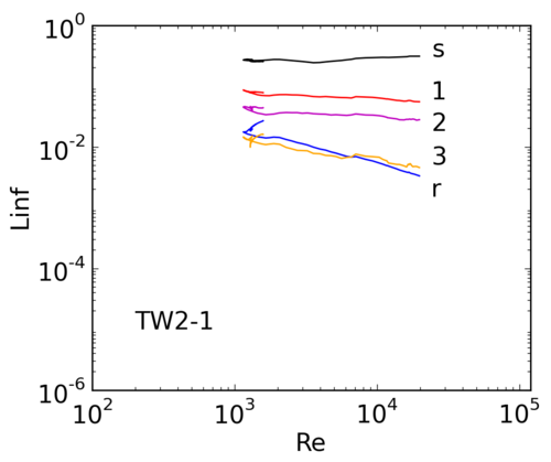
Figure 13: Scaling of streamwise Fourier modes of plane Couette and channel solutions. (a,b,c) Spatially periodic plane Couette equilibria NBCW, EQ7, EQ8, at $\alpha,\gamma=1,2$. (d,e,f) Spatially periodic channel flow traveling waves TW1, TW2, TW3, at $\alpha,\gamma=1,2$. (g,h,i) Spanwise localized solutions: EQ7-1 plane Couette equilibrium and TW1-1 and TW2-1 channel flow traveling wave, at $\alpha=1$. The magnitude of various Fourier components of the velocity, as measured by inf-norm is plotted against Reynolds number. The labels s,r,1,2,3 indicate the streaks $\hat{u}_{0}$, rolls $[\hat{v}_{0},\hat{w}_{0}]$, and the 1st, 2nd, and 3rd streamwise Fourier harmonics $\hat{{\bf u}}_{1}$, $\hat{{\bf u}}_{2}$, and $\hat{{\bf u}}_{3}$. The vertical axis is the $\infty$-norm of the given component (see text).

$j$		NBCW	EQ7	EQ7-1	EQ7-2	TW1	TW1-1	TW1-2
$0$	streak	$0.01$	$0.10$	$0.14$	$0.12$	$0.06$	$0.08$	$0.09$
$1$	wave	$0.85$	$0.77$	$0.90$	$0.83$	$0.80$	$0.80$	$0.82$
$0$	roll	$1.0$	$0.97$	$1.0$	$1.0$	$1.05$	$1.02$	$1.00$
$2$		$1.4$	$1.25$	$1.4$	$1.35$	$1.35$	$1.4$	$1.35$
$3$		$2.2$	$2.6$	$2.25$	$2.45$	$1.95$	$2.2$	$2.0$

Table 2: Scaling exponents for streamwise Fourier harmonics of equilibrium and traveling wave solutions of plane Couette and channel flow. Components of solutions ${\bf u}$ scale as $||\cdot||_{\infty}=O(Re^{-\mu})$ for the given values of $\mu$.

Figure 13 shows the scaling with Reynolds number of the magnitude of the streaks, rolls, waves, and second and third harmonics for a number of plane Couette and channel solutions. The magnitude is computed with the inf-norm; for example, the magnitude $||\hat{{\bf u}}_{1}||_{\infty}$ of the wave is the maximum over $x,y,z$ and the vector components $[u,v,w]$ of ${\bf u}=\hat{{\bf u}}_{1}(y,z)e^{i\alpha x}+\hat{{\bf u}}_{-1}(y,z)e^{-i\alpha x}$. A number of these solutions exhibit very clear scaling of the form $||\hat{{\bf u}}_{j}||_{\infty}=O(Re^{-\mu_{j}})$. For example Figure 13(a) shows that for NBCW, the streaks are $O(1)$, the rolls $O(Re^{-1})$, and the waves $O(Re^{-0.85})$. The streak and roll values scalings equal the theoretical predictions of Hall & Sherwin (2010), and the wave scaling is within 2%. Note that the choice of inf-norm changes the scaling exponent for the NBCW wave component compared to the value of $\mu_{1}=0.9$ reported by Wang et al. (2007).

EQ7 in figure 13(b) shows equally clear asymptotic scaling with exponents comparable but not equal to those of NBCW. The same is true of all solutions derived from EQ7 by parametric continuation and localization by windowing. Examples of such EQ7-related solutions are shown in figure 13, namely (d) TW1, the spatially periodic traveling wave of channel flow obtained from EQ7 by continuation; (g) EQ7-1, the spanwise localized equilibrium of plane Couette flow obtained by windowing; and (i) TW-1, the spanwise localized traveling wave of channel flow obtained by windowing TW-1. Scaling exponents for these solutions plus EQ7-2 and TW7-2 are listed in table 2. It should be noted that the magnitudes of Fourier harmonics of EQ7 and solutions derived from it are substantially different from those of NBCW. For example, comparison of EQ7 in figure 13(b) to NBCW in (a) shows that EQ7’s streaks are about a factor of three smaller than NBCW’s, and its fundamental harmonic is about a factor of three larger, resulting in an order of magnitude less scale separation between these components.

In contrast, the upper-branch and $y$-asymmetric solutions reported here have no clear asymptotic scaling in streamwise Fourier harmonics and substantially poorer separation of scales, namely figure 13(b) EQ8, the upper branch of EQ7; (e) TW2, a spanwise periodic traveling wave of channel flow obtained from judiciously chosen DNS data; (f) TW3, a higher-wavenumber spanwise periodic traveling wave of channel flow obtained from continuation in $Re$ of TW2; and (i) TW2-1, a spanwise localized traveling wave of channel flow obtained from windowing TW2. TW2-2 (not shown) is similar to TW-1. Among these, none of EQ8, TW2, TW2-1, or TW-2 continue in a straightforward fashion to higher Reynolds number; instead the solutions curves turn around at finite $Re$ and follow complex paths. The same is true for EQ2, the upper branch of NBCW. The numerical evidence thus weighs against the possibility of an asymptotic analysis of these solutions based on streamwise Fourier harmonics.

4.3 Critical layers

The development of critical layers is an important consequence of the separation of scales in the streamwise Fourier modes (Wang et al. (2007) and Hall & Sherwin (2010)). The critical layer is the surface on which the mean streamwise fluid velocity matches the wavespeed, i.e. $\hat{u}_{\text{tot},0}(y,z)=c$. When higher harmonics become negligible and the roll velocities $\hat{v}_{0},\hat{w}_{0}$ are small compared to the streaky streamwise velocity $\hat{u}_{\text{tot},0}$, the equation for the fundamental mode simplifies to

$$\left[i\alpha(\hat{u}_{\text{tot},0}-c)\hat{{\bf u}}_{1}+(\hat{{\bf u}}_{1}\cdot{\bf\nabla}\hat{{\bf u}}_{\text{tot},0}){\bf e}_{x}\right]e^{i\theta}={\bf\nabla}(\hat{p}_{1}e^{i\theta})+Re^{-1}\nabla^{2}(\hat{{\bf u}}_{1}e^{i\theta})$$ (13)

As argued by Wang et al. (2007), for large $Re$ the fundamental harmonic $\hat{{\bf u}}_{1}$ concentrates in a region of thickness $\delta=Re^{-1/3}$ about the critical layer, in which (13) is dominated by a balance between its first and last terms. For a point ${\bf x}$ in this region and ${\bf x}_{c}$ nearby on the critical layer, this requires a balance of $\alpha(\hat{u}_{\text{tot},0}({\bf x})-c)\approx\alpha({\bf x}-{\bf x}_{c})\cdot{\bf\nabla}\hat{{\bf u}}_{\text{tot},0}$ against $Re^{-1}\nabla^{2}$. If $\delta\sim|{\bf x}-{\bf x}_{c}|$ is the thickness of the region, the balance requires $\alpha\delta|{\bf\nabla}\hat{{\bf u}}_{\text{tot},0}|\sim Re^{-1}\delta^{-2}$ or $\delta=(\alpha|{\bf\nabla}\hat{{\bf u}}_{\text{tot},0}|Re)^{-1/3}$.

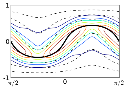
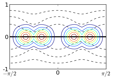
(a)	(c)	(e)
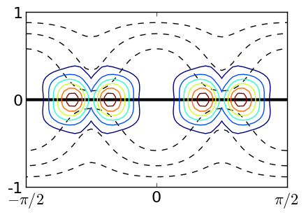
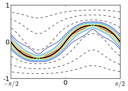
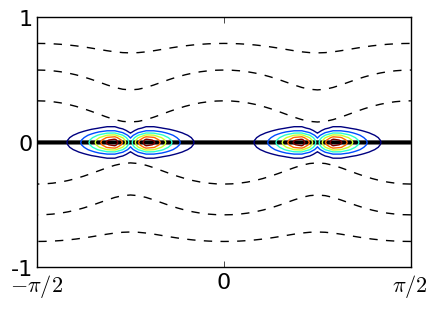
(b)	(d)	(f)

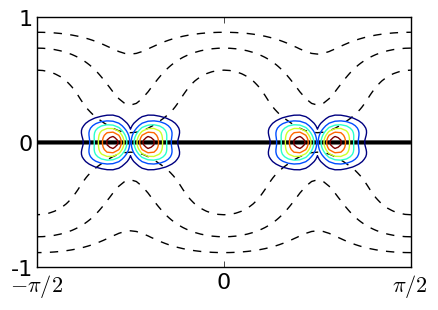
Figure 14: Critical layers of spanwise periodic equilibria of plane Couette flow. (a,b) NBCW at $Re=1000$ and $30000$, (c,d) EQ7 at $Re=1000$ and $30000$, and (e,f) EQ8 at $Re=1000$ and $3000$ for streamwise, spanwise wavenumbers $\alpha,\gamma=1,2$. Dashed contour lines show total streamwise velocity at levels $u_{\text{tot}}=\pm\{0,0.25,0.50,0.75\}$. The critical layer where $u_{\text{tot}}(y,z)=c=0$ is shown with a thick solid contour line. Thin solid contour lines show the autoscaled magnitude of the fundamental Fourier harmonic, $|\hat{{\bf u}}_{1}|$. The horizontal and vertical coordinates are $z,y$ respectively.

Figure 14 illustrates the development of the critical layer for three spatially periodic equilibria of plane Couette flow. For equilibria, the wavespeed vanishes, so the critical layer in these plots is the surface $y=f(z)$ on which $u_{\text{tot}}(y,z)=0$. For NBCW, shown in figure 14(a,b), the height of the critical layer varies in $z$, and its thickness $\delta$ decreases as $Re^{-1/3}$ between (a) $Re=1000$ and (b) $Re=30000$. Figure 14(a,b) largely duplicates figures 2 and 3 of Wang et al. (2007); however we note that our plots show contourlines of $|\hat{{\bf u}}_{1}|$ rather than just the vertical component, $|\hat{v}_{1}|$, and so more clearly convey the fact that, for NBCW, the concentration of the fundamental mode is spread almost uniformly over the entire critical layer.

The critical layers for EQ7 and its upper branch EQ8 are markedly different (figure 14(c,d) and (e,f)). First, the critical layer for these solutions is the line $y=0$. This follows from their $\sigma_{xy}$ symmetry, i.e. $[u,v,w](x,y,z)=[-u,-v,w](-x,-y,z)$. Under this symmetry the $x$-average of the perturbation velocity and total velocity vanishes on $y=0$. We note that some of the complexity of Hall & Sherwin (2010)’s analysis results from the need to work in a coordinate system aligned with the curved criticial layer; for EQ7 and EQ8 this complexity would be eliminated. Second, the fundamental mode $\hat{{\bf u}}_{1}$ concentrates not uniformly over the whole critical layer, but apparently on isolated spots within it. Third, EQ8 seems to form a critical layer at $Re=2000$, even though its scale separation is much poorer and its large-$Re$ limit apparently does not exist.

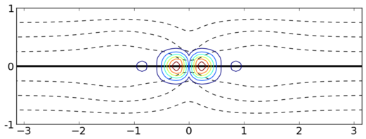
(a)	(c)
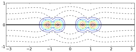
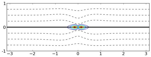
(b)	(d)

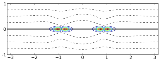
Figure 15: Critical layers of spanwise localized equilibria of plane Couette flow. (a,b) EQ7-1 at $Re=1000$ and $30000$ and (c,d) EQ7-2 at $Re=1000$ and $30000$ for streamwise wavenumber $\alpha=1$, with $y$ vertical and $z$ horizontal. Plotting conventions are the same as figure 14. The $z\in[-\pi,\pi]$ subset of the full $[-3\pi,3\pi]$ computational domain is shown.

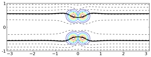
(a)	(c)
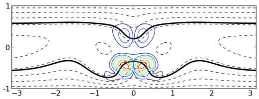
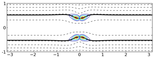
(b)	(d)

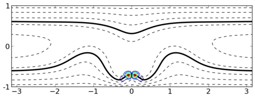
Figure 16: Critical layers of spanwise localized traveling waves of channel flow. (a,b) TW1-1 at $Re=2000$ and $30000$ and (c,d) TW2-1 at $Re=2000$ and $20000$ for streamwise wavenumber $\alpha=1$, with $y$ vertical and $z$ horizontal. Plotting conventions are the same as figure 14 except total streamwise velocity contours are shown at levels $u_{\text{tot}}=\{0.1,0.3,0.5,0.7,0.9\}$. The $z\in[-\pi,\pi]$ subset of the full $[-3\pi,3\pi]$ computational domain is shown.

Figure 15 shows that the critical layer structure of EQ7 carries over directly to its spanwise-localized counterparts EQ7-1 and EQ7-2, with tapering to laminar flow at large $|z|$. In particular the isolated concentrations $\hat{{\bf u}}_{1}$ on the critical layer can be seen, by comparison with figure 4, to result from the first-harmonic $x$ variations of the $y,z$-localized and concentrated vortex structures. Figure 16(a,b) shows that EQ7 and EQ7-1’s critical layer structure carries over to TW1-1, in two copies mirrored symmetrically about $y=0$. The channel traveling waves have a nonzero wavespeed $c$ and lack EQ7’s $\sigma_{xy}$ symmetry, and therefore have a critical layer $\hat{u}_{\text{tot},0}(y,z)-c=0$ whose height varies in $z$.

Figure 16(c,d) shows critical layer development for the $y$-asymmetric channel traveling wave TW2-1. Note that $y$-asymmetry increases while $y$ and $z$ length scales decrease with increasing $Re$. In particular, $\hat{{\bf u}}_{1}$ concentrates in a smaller region that approaches the wall as $Re$ increases. An obvious question is whether this represents a near-wall coherent structure that is constant in wall units. We intend to address this question in future work. For the time being we note that the behavior illustrated in figure 16(c,d) is still subject to a prescribed length scale in the form of the streamwise wavelength $\alpha$, and that this prescription must be removed, by streamwise localization or proper scaling with $Re$, in order for the lengthscales to be determined naturally.

5 Conclusions

We have found a number of new spanwise-localized equilibrium solutions of plane Couette flow and traveling-wave solutions of channel flow, and additionally a few spanwise periodic solutions of channel flow incidental to the construction of the localized solutions. The spanwise localized solutions consist of a core region that closely resembles a spanwise periodic solution, a transition region, and exponentially decaying tails. The decay rate of the tails is $e^{-\alpha|z|}$, and their structure is determined by solely by the streamwise wavenumber, the laminar flow profile, and the wavespeed, and is otherwise independent of the structure of the core region. The solutions related to Itano & Generalis (2009) and Gibson et al. (2009)’s HSV/EQ7 display clear scale separation and asymptotic scaling in streamwise Fourier harmonics, suggesting that they are amenable to analysis via a reduced-order PDE retaining only a few harmonics.

Several solutions, namely TW2-1 and TW2-2, capture particularly isolated and elemental exact coherent structures in the near-wall of shear flows, which suggestively resemble the lambda vortices that form in spatially developing flows. These solutions consist of long bands of concentrated vortices near the walls, with alternating orientation, and roughly aligned with the streamwise axis but tilting slightly in the spanwise and wall-normal directions. The concentrated vortices near the walls are flanked by small high-speed streaks very near the walls and otherwise surrounded by very large regions where the streamwise velocity is reduced relative to the laminar background. These solutions capture, as exact time-independent solutions of Navier-Stokes, the process by which near-wall vortices exchange momentum between the near-wall and core regions of wall-bounded shear flows and thereby increase drag.

Acknowledgments. The authors thank Tobias Schneider, Greg Chini, Spencer Sherwin, and Philip Hall for illuminating discussions.

References

- Adrian (2007) Adrian, R. 2007 Hairpin vortex organization in wall turbulence. Phys. Fluids 19, 041301.
- Aubry et al. (1988) Aubry, N., Holmes, P., Lumley, J. L. & Stone, E. 1988 The dynamics of coherent structures in the wall region of turbulent boundary layer. J. Fluid Mech. 192, 115–173.
- Burke & Knobloch (2007) Burke, J. & Knobloch, E. 2007 Homoclinic snaking: Structure and stability. Chaos 17 (3), 037102.
- Canuto et al. (2006) Canuto, C., Hussaini, M. Y., Quarteroni, A. & Zang, T. A. 2006 Spectral Methods: Fundamentals in Single Domains. Springer.
- Chandler & Kerswell (2013) Chandler, G.J. & Kerswell, R.R. 2013 Simple invariant solutions embedded in 2D Kolmogoov turbulence. J. Fluid Mech 722, 554–595.
- Clever & Busse (1992) Clever, R. M. & Busse, F. H. 1992 Three-dimensional convection in a horizontal layer subjected to constant shear. J. Fluid Mech. 234, 511–527.
- Cvitanović & Gibson (2010) Cvitanović, P. & Gibson, J. F. 2010 Geometry of turbulence in wall-bounded shear flows: Periodic orbits. Phys. Scr. T 142, 014007.
- Duguet et al. (2008) Duguet, Y., Pringle, C. C. T. & Kerswell, R. R. 2008 Relative periodic orbits in transitional pipe flow. Phys. Fluids 20, 114102, arXiv:0807.2580.
- Duguet et al. (2009) Duguet, Y., Schlatter, P. & Henningson, D. 2009 Localized edge states in plane Couette flow. Phys. Fluids 21, 111701.
- Faisst & Eckhardt (2003) Faisst, H. & Eckhardt, B. 2003 Traveling waves in pipe flow. Phys. Rev. Lett. 91, 224502.
- Gibson (2013) Gibson, J. F. 2013 Channelflow: a spectral Navier-Stokes simulator in C++. Tech. Rep.. Univ. New Hampshire, www.channelflow.org.
- Gibson et al. (2008) Gibson, J. F., Halcrow, J. & Cvitanović, P. 2008 Visualizing the geometry of state space in plane Couette flow. J. Fluid Mech. 611, 107–130, arXiv:0705.3957.
- Gibson et al. (2009) Gibson, J. F., Halcrow, J. & Cvitanović, P. 2009 Equilibrium and traveling-wave solutions of plane Couette flow. J. Fluid Mech. 638, 1–24, arXiv:0808.3375.
- Halcrow et al. (2009) Halcrow, J., Gibson, J. F., Cvitanović, P. & Viswanath, D. 2009 Heteroclinic connections in plane Couette flow. J. Fluid Mech. 621, 365–376, arXiv:0808.1865.
- Hall & Sherwin (2010) Hall, P. & Sherwin, S. 2010 Streamwise vortices in shear flows: harbingers of transition and the skeleton of coherent structures. J. Fluid Mech. 661, 178–205.
- Hamilton et al. (1995) Hamilton, J. M., Kim, J. & Waleffe, F. 1995 Regeneration mechanisms of near-wall turbulence structures. J. Fluid Mech. 287, 317–348.
- Hof et al. (2004) Hof, B., van Doorne, C. W. H., Westerweel, J., Nieuwstadt, F. T. M., Faisst, H., Eckhardt, B., Wedin, H., Kerswell, R. R. & Waleffe, F. 2004 Experimental observation of nonlinear traveling waves in turbulent pipe flow. Science 305, 1594–1598.
- Holmes et al. (1996) Holmes, P., Lumley, J. L. & Berkooz, G. 1996 Turbulence, coherent structures, dynamical systems and symmetry. Cambridge: Cambridge University Press.
- Hoyle (2006) Hoyle, R. 2006 Pattern Formation: An Introduction to Methods. Cambridge: Cambridge Univ. Press.
- Itano & Generalis (2009) Itano, T. & Generalis, S. C. 2009 Hairpin vortex solution in planar Couette flow: A tapestry of knotted vortices. Phys. Rev. Lett. 102, 114501.
- Itano & Toh (2001) Itano, T. & Toh, S. 2001 The dynamics of bursting process in wall turbulence. J. Phys. Soc. Japan 70, 701–714.
- Kawahara & Kida (2001) Kawahara, G. & Kida, S. 2001 Periodic motion embedded in plane Couette turbulence: Regeneration cycle and burst. J. Fluid Mech. 449, 291–300.
- Kawahara et al. (2012) Kawahara, G., Uhlmann, M. & van Veen, L. 2012 The significance of simple invariant solutions in turbulent flows. Annual Review of Fluid Mechanics 44, 203–225.
- Lorenz (1963) Lorenz, E. N. 1963 Deterministic nonperiodic flow. J. Atmos. Sci. 20, 130.
- de Lozar et al. (2012) de Lozar, A., Mellibovsky, D., Avila, M. & Hof, B. 2012 Edge state in pipe flow experiments. Phys. Rev. Lett. 108, 214502.
- Nagata (1990) Nagata, M. 1990 Three-dimensional finite-amplitude solutions in plane Couette flow: bifurcation from infinity. J. Fluid Mech. 217, 519–527.
- Nagata (1997) Nagata, M. 1997 Three-dimensional traveling-wave solutions in plane Couette flow. Phys. Rev. E 55, 2023–25.
- Okino et al. (2010) Okino, S., Nagata, M., Wedin, H. & Bottaro, A. 2010 A new nonlinear vortex state in square-duct flow. J. Fluid Mech. 657, 413–29.
- Peyret (2002) Peyret, R. 2002 Spectral Methods for Incompressible Flows. Springer.
- Saiki et al. (1993) Saiki, E.M., Biringen, S., Danablasoglu, G. & Streett, C.L. 1993 Spatial simulation of secondary instability in plane channel flow: comparison of k- and h-type disturbances. J. Fluid Mech. 253, 485–507.
- Schmiegel (1999) Schmiegel, A. 1999 Transition to turbulence in linearly stable shear flows. PhD thesis, Philipps-Universität Marburg, available on archiv.ub.uni-marburg.de/diss/z2000/0062.
- Schneider et al. (2010) Schneider, T. M., Gibson, J. F. & Burke, J. 2010 Snakes and ladders: Localized solutions of plane Couette flow. Phys. Rev. Lett. 104, 104501.
- Schneider et al. (2008) Schneider, T. M., Gibson, J. F., Lagha, M., Lillo, F. De & Eckhardt, B. 2008 Laminar-turbulent boundary in plane Couette flow. Phys. Rev. E. 78, 037301, arXiv:0805.1015.
- Schneider et al. (2009) Schneider, T. M., Marinc, D. & Eckhardt, B. 2009 Localized edge states nucleate turbulence in extended plane Couette cells. J. Fluid Mech. p. in press.
- Spalart et al. (1991) Spalart, P. R., Moser, R. D. & Rogers, M. M. 1991 Spectral methods for the Navier-Stokes equations with one infinite and two periodic directions. J. Comp. Physics 96, 297–324.
- van Veen & Kawahara (2011) van Veen, L. & Kawahara, G. 2011 Homoclinic tangle on the edge of shear turbulence. Phys. Rev. Lett. 107, 114501.
- Viswanath (2007) Viswanath, D. 2007 Recurrent motions within plane Couette turbulence. J. Fluid Mech. 580, 339–358.
- Viswanath (2009) Viswanath, D. 2009 The critical layer in pipe flow at high Reynolds number. Phil. Trans. R. Soc. A 367, 561–576.
- Waleffe (1997) Waleffe, F. 1997 On a Self-Sustaining Process in shear flows. Phys. Fluids 9, 883–900.
- Waleffe (1998) Waleffe, F. 1998 Three-dimensional coherent states in plane shear flows. Phys. Rev. Lett. 81, 4140–4143.
- Waleffe (2001) Waleffe, F. 2001 Exact coherent structures in channel flow. J. Fluid Mech. 435, 93–102.
- Waleffe (2003) Waleffe, F. 2003 Homotopy of exact coherent structures in plane shear flows. Phys. Fluids 15, 1517–1534.
- Wang et al. (2007) Wang, J., Gibson, J. F. & Waleffe, F. 2007 Lower branch coherent states in shear flows: Transition and control. Phys. Rev. Lett. 98 (20), 204501.
- Wedin & Kerswell (2009) Wedin, H. & Kerswell, R.R. 2009 Three-dimensional traveling waves in a square duct. Phys. Rev. E 79, 065305.
- Zhou et al. (1999) Zhou, J., Adrian, R.J., Balachandar, S. & Kendall, T.M. 1999 Mechanisms for generating coherent packets of hairpin vortices in channel flow. J. Fluid Mech. 387, 353–396.