Efficient tomography of quantum-optical Gaussian processes probed with a few coherent states

Abstract

An arbitrary quantum-optical process (channel) can be completely characterized by probing it with coherent states using the recently developed coherent-state quantum process tomography (QPT) [Lobino et al., Science 322, 563 (2008)]. In general, precise QPT is possible if an infinite set of probes is available. Thus, realistic QPT of infinite-dimensional systems is approximate due to a finite experimentally-feasible set of coherent states and its related energy-cut-off approximation. We show with explicit formulas that one can completely identify a quantum-optical Gaussian process just with a few different coherent states without approximations like the energy cut-off. For tomography of multimode processes, our method exponentially reduces the number of different test states, compared with existing methods.

I Introduction

One of the basic problems of quantum physics is to predict the evolution of a quantum system under certain conditions. For an isolated system with a known Hamiltonian, the evolution is characterized by a unitary operator determined by the Schrödinger equation. However, the system may interact with its environment, and the total Hamiltonian of the system plus the environment is in general not completely known. The evolution can then be regarded as a “black-box process” Poyatos97 ; Chuang97 ; DAriano01 which maps the input state into an output state. An important problem here is how to characterize an unknown process by testing the black-box with some specific input states, which is referred to as quantum process tomography (QPT) (for reviews see Refs. Paris04 ; Mohseni08 ).

QPT can be understood as the tomography of a quantum channel since any physical operation describing the dynamics of a quantum state can be considered as a channel Eisert05 . In contrast, the goal of quantum state tomography (QST) is the reconstruction of an unknown state (i.e., its density matrix) by a series of measurements on multiple copies of the state (for a review see Ref. Paris04 ). Both QPT and QST are essential tools in quantum engineering and quantum information processing.

A few methods for QPT were developed, including the standard QPT Chuang97 ; Poyatos97 , ancilla-assisted QPT DAriano01 ; Leung03 ; Altepeter03 ; DAriano03 , direct characterization of quantum dynamics Mohseni06 ; Wang07 , and coherent-state QPT Lobino08 . There are dozens of proposals and experimental realizations of QPT for systems with a few qubits. These include the estimation of quantum-optical gates Altepeter03 ; Mitchell03 ; Demartini03 ; Obrien04 ; Nambu05 ; Langford05 ; Kiesel05 ; Wang07 ; Ma12 , liquid nuclear-magnetic-resonance gates Childs01 ; Boulant03 ; Weinstein04 , superconducting gates Liu04 ; Zagoskin06 ; Neeley08 ; Chow09 ; Bialczak10 ; Chow12 (for a review see Ref. You11 ) and other solid-state gates Kampermann05 ; Howard06 ; Burgarth11 , ion-trap gates Riebe06 ; Monz09 , or the estimation of the dynamics of atoms in optical lattices Myrskog05 . In contrast, there are only a very few experimental demonstrations of QPT for infinite-dimensional systems (see, e.g., Ref. Lobino08 ).

Any physical process can be described by a completely positive map $\varepsilon$. Such a process is fully characterized if the evolution of any input state $\rho_{\rm in}$ is predictable: $\rho_{\rm out}=\varepsilon(\rho_{\rm in})$. In general, QPT is very difficult to implement in high-dimensional spaces, and, more challengingly, in an infinite-dimensional space, such as a Fock space DAriano03 ; Lobino08 . Recently, Ref. Lobino08 described QPT in a Fock space for continuous variable (CV) states. Two conclusions can be drawn Lobino08 : ($i$) If the output states of all coherent input states are known, then one can predict the output state of any input state; ($ii$) By taking the photon-number-cut-off (or energy cut-off) approximation, one can then characterize an unknown process with a finite number of different input coherent states (CSs).

It is an interesting question to identify an exact QPT with a finite number of coherent states. If the process is completely unknown, then QPT with a finite number of coherent states is impossible. However, if some of the constraints of the quantum process are known, then QPT can be simplified and, thus, effective. Gaussian maps are the most common for quantum-optical processes. In this article, we show that if a certain quantum process is known to be Gaussian, then an exact QPT can be performed with only a few different coherent states.

It is worth noting that there is an analogy between QPT and QST, especially for quantum-optical Gaussian processes (channels) Eisert05 ; Holevo12 and Gaussian states Holevo11 ; Rehacek09 . This analogy can be seen, e.g., by comparing correlations between observables encoded in the covariance matrices, which completely describe a Gaussian object (either a quantum state or process). Thus, tomographies of quantum Gaussian systems are effectively finite-dimensional with their covariance matrix having a physical meaning analogous to a finite-dimensional density matrix.

As has been shown in Ref. DAriano01 , QPT can be performed with two-mode squeezed vacuum (TMSV) for any unknown process. However, TMSVs are not so easy to manipulate in practice, especially, because this involves quantum tomography of entangled states, which is not an easy task.

Here, we show that based on existing results DAriano01 , by using the standard quantum-optical Husimi $Q$-representation, one can perform QPT with only a few CSs without entangled ancillas for quantum-optical Gaussian processes. The method described here has several advantages. First, it presents explicit formulas without any approximations, such as the photon-number-cut-off approximation. Second, it requires only a few different states to characterize a process, rather than all CSs. Third, for multimode Gaussian process tomography, the number of input CSs increases polynomially with the number of modes, rather than exponentially. Fourth, it uses the Husimi $Q$-functions only, which is always well-defined for any state without any higher-order singularities in the calculation.

The paper is organized as follows: We review the existing results about QPT based on entangled ancillas in Sec. II. In Sec. III, the QPT without ancillas is proposed for single-mode Gaussian processes. A simple illustrative example of the method is discussed in Sec. III.A. A generalization of our QPT for a multi-mode case is presented in Sec. IV. We conclude in Sec. V.

II Ancilla-assisted quantum process tomography

First, we review the existing result of the ancilla-assisted QPT with TMSV DAriano01 to show some similarities but also crucial differences in comparison to our proposal of ancilla-free QPT, which will be described in Sec. III.

A TMSV is defined by $|\chi(q)\rangle=c_{q}\exp({qa^{\dagger}b^{\dagger}})|00\rangle$, where $c_{q}=\sqrt{1-q^{2}}$, and $q$ is real. The (unnormalized) maximally-entangled state here is

$$|\Phi^{+}\rangle=\lim_{q\rightarrow 1}\exp(qa^{\dagger}b^{\dagger})|00\rangle=\sum_{k=0}^{\infty}|kk\rangle,$$ (1)

where $a^{\dagger}$ ($b^{\dagger}$) is the creation operator for mode $a$ ($b$). Note that entanglement is not required for the ancilla-assisted QPT, but it makes it more efficient. In particular, the use of the maximally-entangled states can make the QPT experimentally optimal with regard to perfect nonlocal correlations Altepeter03 .

Assume now that the black box process acts only in mode $b$ of the bipartite state $|\chi(q)\rangle$. After the process, we obtain a two-mode state $\Omega_{q}$. One can define the projection operator

$$T(q)=c_{q}\exp[(\ln q)a^{\dagger}a],$$ (2)

which has the property Louisell73 :

$$T(q)\;(a,a^{\dagger})\;T^{-1}(q)=(a/q,qa^{\dagger}).$$ (3)

The TMSV $|\chi(q)\rangle$ can be written as

$$|\chi(q)\rangle=T(q)\otimes I|\Phi^{+}\rangle.$$ (4)

According to Eq. (4), we have

$$\Omega_{q}=T(q)\otimes I\cdot\rho_{\varepsilon}\cdot T(q)\otimes I,$$ (5)

where $\rho_{\varepsilon}=I\otimes\varepsilon\left(|\Phi^{+}\rangle\langle\Phi^{+}|\right)$. Naturally,

$$\rho_{\varepsilon}=T^{-1}(q)\otimes I\cdot\Omega_{q}\cdot T^{-1}(q)\otimes I.$$ (6)

We now also formulate the output state of any single-mode input state $|\psi(\{c_{k}\})\rangle=\sum_{k}c_{k}|k\rangle$ of mode $b$. Obviously it can be written as

$$\left(|\psi\rangle\langle\psi|\right)_{b} = {{}_{a}}\langle\psi^{*}|\Phi^{+}\rangle\langle\Phi^{+}|\psi^{*}\rangle_{a}$$ (7)

$$= {\rm tr_{a}}\left(|\psi^{*}\rangle\langle\psi^{*}|\otimes I\cdot|\Phi^{+}\rangle\langle\Phi^{+}|\right),$$

and $|\psi^{*}\rangle_{a}=\sum_{k}c_{k}^{*}|k\rangle_{a}$ is a single-mode state for mode $a$ (sometimes we omit the subscript $a$ or $b$ for simplicity). We obtain the output state

$$\rho_{\psi} = {{}_{a}\langle\psi^{*}|\rho_{\epsilon}|\psi^{*}\rangle_{a}=\rm{tr}_{a}(|\psi^{*}\rangle\langle\psi^{*}|\otimes I\cdot\rho_{\epsilon})}$$ (8)

$$= {\rm tr_{a}}\left[|\psi^{*}(\{c_{k}/q^{k}\})\rangle\langle\psi^{*}(\{c_{k}/q^{k}\})|\otimes I\cdot\Omega_{q}\right]$$

$$= {{}_{a}\langle\psi^{*}(\{c_{k}/q^{k}\})|\Omega_{q}|\psi^{*}(\{c_{k}/q^{k}\})\rangle_{a}}.$$

More explicit expressions can be obtained by using the Husimi $Q$-function. If the single-mode input state in mode $b$ is a coherent state $|\alpha\rangle$, the output state then becomes

$$\rho_{\alpha}=\langle\alpha^{*}|\rho_{\varepsilon}|\alpha^{*}\rangle=\langle\alpha^{*}|T^{-1}(q)\otimes I\cdot\Omega_{q}\cdot T^{-1}(q)\otimes I|\alpha^{*}\rangle.$$ (9)

Note that the state $|\alpha^{*}\rangle$ here is a single-mode coherent state in mode $a$. Using the property of $T(q)$ and the definition of CSs, $a|\alpha^{*}\rangle=\alpha^{*}|\alpha^{*}\rangle$, we easily find

$$T^{-1}(q)\otimes I\;|\alpha^{*}\rangle=\mathcal{N}_{q}(\alpha)\;|\alpha^{*}/q\rangle,$$ (10)

where the factor $\mathcal{N}_{q}(\alpha)=\exp\left[-|\alpha|^{2}(1-1/q^{2})/2\right]/c_{q}$, and $|\alpha^{*}/q\rangle$ is a coherent state in mode $a$ defined by $a|\alpha^{*}/q\rangle=(\alpha^{*}/q)|\alpha^{*}/q\rangle$. Thus, the output state of mode $b$ is

$$\rho_{\alpha}=|\mathcal{N}_{q}(\alpha)|^{2}\;{{}_{a}\langle\alpha^{*}/q\;|\Omega_{q}\;|\alpha^{*}/q\rangle_{a}}\,.$$ (11)

Let $|Z_{a},Z_{b}\rangle$ be a two-mode coherent state defined by $(a,b)|Z_{a},Z_{b}\rangle=(Z_{a},Z_{b})|Z_{a},Z_{b}\rangle$, where $Z_{a},Z_{b}$ are complex amplitudes. Then, the Husimi $Q$-function for $\Omega_{q}$ can be defined as

$$Q_{\Omega_{q}}(Z_{a}^{*},Z_{b}^{*},Z_{a},Z_{b})=\langle Z_{a},Z_{b}|\Omega_{q}|Z_{a},Z_{b}\rangle,$$ (12)

and the corresponding density operator is the following normally-ordered operator

$$\Omega_{q}=:Q_{\Omega_{q}}(a^{\dagger},b^{\dagger},a,b):\;,$$ (13)

which is simply the operator functional obtained by replacing the variables $(Z_{a}^{*},Z_{b}^{*},Z_{a},Z_{b})$ with $(a^{\dagger},b^{\dagger},a,b)$ in the $Q$-function given by Eq. (12), analogously to Eq. (21). Therefore, using Eq. (11) and the normally-ordered form of $\Omega_{q}$, we have the following simple form for the Husimi $Q$-function

$$Q_{\rho_{\alpha}}({Z_{b}}^{*},Z_{b})=|N_{q}(\alpha)|^{2}Q_{\Omega_{q}}({\alpha}/{q},{Z_{b}}^{*},{\alpha^{*}}/{q},Z_{b})$$ (14)

of the output state $\rho_{\alpha}$. Eqs. (11)-(14) are the explicit expressions of the output state for the input of any coherent state $|\alpha\rangle$. According to Ref. Lobino08 , if we know the output states for all input CSs, then we know the output states of all states in Fock space. In this approach, given any input state $|\psi\rangle$, we can write it in its linear superposition form in the coherent-state basis, and then obtain the $Q$-function of its output state by using Eq. (14).

These results can be generalized for a multimode QPT. To apply the Jamiolkowski isomorphism Jamiolkowski72 , we consider $k$ pairs of maximally-entangled states, each in modes $a_{1},b_{1}$, $a_{2},b_{2}$,$\cdots$, $a_{k},b_{k}$. Explicitly, $|\Phi^{+}\rangle=|\phi^{+}\rangle_{1}|\phi^{+}\rangle_{2}\cdots|\phi^{+}\rangle_{k}.$ Here $|\phi^{+}\rangle_{i}=\lim_{q\rightarrow 1}\exp({qa_{i}^{\dagger}b_{i}^{\dagger}})|00\rangle$ indicates a maximally-entangled state in modes $a_{i},\;b_{i}$. Subspaces $a$ and $b$ each are now $k$-mode. Any state $|\psi\rangle$ in subspace $b$, can still be written in the form of Eq. (7), with the new definitions for $|\psi\rangle$ and $|\Phi^{+}\rangle$. Using Eq. (6), it is obvious that the output state of these $k$-pairs of TMSV fully characterizes the process.

III Ancilla-free Gaussian process tomography with a few coherent states

Now we present the main result of this paper, which is an efficient tomography of Gaussian processes probed with only a few single-mode coherent states without the assistance of ancillas.

As shown in Ref. Lobino08 , if we only use CSs in the test, the tomography of an unknown process in Fock space requires tests with all CSs. Though this problem can be solved by taking the photon-number-cut-off approximation, in a quantum-optical process associated with intense light, one still needs a huge number of different CSs for the test. Here we show that the most important process in quantum optics, the Gaussian process Eisert05 ; Holevo12 , can be exactly characterized with only a few CSs in the test.

A Gaussian process maps Gaussian states into Gaussian states Eisert02 . Therefore the Husimi $Q$-function of the operator $\rho_{\varepsilon}$ must be Gaussian:

$$Q_{\rho_{\varepsilon}}(Z_{a}^{*},Z_{b}^{*},Z_{a},Z_{b})=\exp(c_{0}+L+L^{\dagger}+S+S^{\dagger}+S_{0}),$$ (15)

where

$$L = (\Gamma_{a},\Gamma_{b})\left(\begin{array}[]{c}Z_{a}\\ Z_{b}\end{array}\right),$$

$$S = \frac{1}{2}(Z_{a},Z_{b})X\left(\begin{array}[]{c}Z_{a}\\ Z_{b}\end{array}\right),$$

$$S_{0} = (Z_{a}^{*},Z_{b}^{*})Y\left(\begin{array}[]{c}Z_{a}\\ Z_{b}\end{array}\right),$$

$$X = X^{T}=\left(\begin{array}[]{cc}X_{aa}&X_{ab}\\ X_{ba}&X_{bb}\end{array}\right),$$

$$Y = Y^{\dagger}=\left(\begin{array}[]{cc}Y_{aa}&Y_{ab}\\ Y_{ba}&Y_{bb}\end{array}\right).$$

Before testing the map, all these are unknowns. The normally-ordered form of the density operator $\rho_{\varepsilon}$ is

$$\rho_{\varepsilon}=:Q_{\rho_{\varepsilon}}(a^{\dagger},b^{\dagger},a,b):$$ (21)

corresponding to Eq. (15) but with variables $(Z_{a}^{*},Z_{b}^{*},Z_{a},Z_{b})$ replaced by $(a^{\dagger},b^{\dagger},a,b)$. The normal order notation $:\ldots:$ indicates that any term inside it is reordered by placing the creation operator in the left. For example, $:aba^{\dagger}b^{\dagger}a:=a^{\dagger}b^{\dagger}a^{2}b$.

The output state from any single-mode input coherent state $|u\rangle$ (in mode $b$) is

$$\rho_{u}={\rm tr}_{a}\left[\left(|u^{*}\rangle\langle u^{*}|\right)_{a}\otimes I\cdot\rho_{\varepsilon}\right],$$ (22)

where $\rho_{\varepsilon}$ is given by Eq. (21). Its Husimi $Q$-function is

$$Q_{\rho_{u}}(Z_{b}^{*},Z_{b}) = Q_{\rho_{\varepsilon}}(u,Z_{b}^{*},u^{*},Z_{b})$$ (23)

$$= \exp(c_{u}+L_{u}+L_{u}^{\dagger}+R+R^{\dagger}+{R_{0}}),\hskip 19.91692pt$$

where

$$L_{u}=(\Gamma_{b}+u^{*}X_{ab}+uY_{ab})Z_{b},$$

$$R=Z_{b}X_{bb}Z_{b}/2,\quad{R_{0}}=Z_{b}^{*}Y_{bb}Z_{b},$$

and $c_{u}$ is determined by $c_{0}$, $\Gamma_{a}$, $X_{aa}$, and $Y_{aa}$. Explicitly,

$$c_{u}=c_{0}+{\rm Re}\left(2\Gamma_{a}u^{*}+u^{*}X_{aa}u^{*}+uY_{aa}u^{*}\right).$$ (24)

The quadratic functional terms ($R,R^{\dagger},R_{0}$) in the exponent in Eq. (23) are independent of $u$; these terms must be the same for the output states from any input CSs. Therefore, these can be known by testing the map with one coherent state. Thus, we do not need to consider these terms below.

Now suppose that we test the process with six different CSs, $|\alpha_{i}\rangle$, and $i=1,2,\cdots,6$. Assume also that the detected Husimi $Q$-function of the output states is

$$Q_{\rho_{\alpha_{i}}}(Z^{*}_{b},Z_{b})=\exp(c_{i}+D_{i}+D_{i}^{\dagger}+R+R^{\dagger}+{R_{0}}),$$ (25)

where $D_{i}=d_{i}Z_{b}$ is the detected (hence known) linear term. We note that there are available efficient methods of Gaussian QST based on homodyne detection, which enable the estimation of the Wigner function or, equivalently, the Husimi $Q$-function for Gaussian states Rehacek09 . According to Eq. (23), the $Q$-function of the output state from the initial state $|\alpha_{i}\rangle$ of mode $b$ must be

$$Q_{\rho_{\alpha_{i}}}(Z^{*}_{b},Z_{b})=Q_{\rho_{\varepsilon}}(\alpha_{i},Z_{b}^{*},{\alpha_{i}}^{*},Z_{b}).$$ (26)

Therefore, we can derive self-consistent equations by using the detected data from $\rho_{\alpha_{i}}$ and setting $u=\alpha_{i}$ in Eq. (23):

$$L_{i}=D_{i},\quad c_{\alpha_{i}}=c_{i},$$ (27)

where $L_{i}$, $c_{\alpha_{i}}$ are just $L_{u}$, $c_{u}$, respectively, after setting $u=\alpha_{i}$ in Eqs. (23)-(24); $D_{i}$ and $c_{i}$ are known from tests. Explicitly,

$$L_{i}=(\Gamma_{b}+{\alpha_{i}}^{*}X_{ab}+{\alpha_{i}}Y_{ab})Z_{b}.$$ (28)

The first part of Eq. (27) causes:

$$K\cdot\left(\Gamma_{b},\;X_{ab},\;Y_{ab}\right)^{T}=d,$$ (29)

where

$$K=\left(\begin{array}[]{ccc}1&{\alpha_{1}}^{*}&\alpha_{1}\\ 1&{\alpha_{2}}^{*}&\alpha_{2}\\ 1&{\alpha_{3}}^{*}&\alpha_{3}\end{array}\right),\quad d=\left(\begin{array}[]{c}d_{1}\\ d_{2}\\ d_{3}\end{array}\right).$$

There are three unknowns ($\Gamma_{b}$, $X_{ab}$, and $Y_{ab}$) with three equations now. We find

$$\left(\Gamma_{b},\;X_{ab},\;Y_{ab}\right)^{T}=K^{-1}d\;.$$ (30)

If the Gaussian process is known to be trace-preserving, then Eq. (30) completes the tomography: up to a numerical factor, we can deduce all the output states of the other input CSs, $|\alpha_{i}\rangle$, for $i=4,5,6$. The term $c_{i}$ can be fixed through normalization, which is determined by the quadratic and linear functional terms in the exponent of the $Q$-functions. Knowing these $\{c_{i}\}$, one can construct $\rho_{\varepsilon}$ completely as shown below.

For any map, $c_{i}$ can be known from tests with $|\alpha_{i}\rangle$, for $i=1,2,\cdots,6$. We then have

$$J\cdot\left(c_{0},\;\Gamma_{a},\;\Gamma^{*}_{a},\;X_{aa},\;X^{*}_{aa},\;Y_{aa}\right)^{T}=c\;,$$ (31)

where

$$J=\left(\begin{array}[]{cccccc}1&\alpha^{*}_{1}&\alpha_{1}&{1\over 2}\alpha^{*2}_{1}&{1\over 2}\alpha^{2}_{1}&|\alpha_{1}|^{2}\\ 1&\alpha^{*}_{2}&\alpha_{2}&{1\over 2}\alpha^{*2}_{2}&{1\over 2}\alpha^{2}_{2}&|\alpha_{2}|^{2}\\ 1&\alpha^{*}_{3}&\alpha_{3}&{1\over 2}\alpha^{*2}_{3}&{1\over 2}\alpha^{2}_{3}&|\alpha_{3}|^{2}\\ 1&\alpha^{*}_{4}&\alpha_{4}&{1\over 2}\alpha^{*2}_{4}&{1\over 2}\alpha^{2}_{4}&|\alpha_{4}|^{2}\\ 1&\alpha^{*}_{5}&\alpha_{5}&{1\over 2}\alpha^{*2}_{5}&{1\over 2}\alpha^{2}_{5}&|\alpha_{5}|^{2}\\ 1&\alpha^{*}_{6}&\alpha_{6}&{1\over 2}\alpha^{*2}_{6}&{1\over 2}\alpha^{2}_{6}&|\alpha_{6}|^{2}\end{array}\right),\;c=\left(\begin{array}[]{c}c_{1}\\ c_{2}\\ c_{3}\\ c_{4}\\ c_{5}\\ c_{6}\end{array}\right),$$

for the second part of Eq. (27). Thus

$$\left(c_{0},\;\Gamma_{a},\;\Gamma^{*}_{a},\;X_{aa},\;X^{*}_{aa},\;Y_{aa}\right)^{T}=J^{-1}c\;.$$ (32)

Theorem: Given $K$ and $J$ defined by Eqs. (29)-(31), then the QPT of any single-mode Gaussian process in Fock space can be performed with six input CSs, when $\det K\not=0$ and $\det J\not=0$. The QPT of any trace-preserving single-mode Gaussian process in Fock space can be executed with three input CSs, when $\det K\not=0$.

For example, one can simply choose $\alpha_{1}=0$, $\alpha_{2}=1$, $\alpha_{3}=i$, $\alpha_{4}=-1$, $\alpha_{5}=-i$, and $\alpha_{6}=1+i$. One finds

$$c_{0} = c_{1},\quad\Gamma_{b}=d_{1},$$

$$\Gamma_{a} = \frac{1}{4}\left(c_{2}+ic_{3}-c_{4}-{i}c_{5}\right),$$

$$X_{ab} = \frac{1}{2}\left[-{(1+i)}d_{1}+d_{2}+{i}d_{3}\right],$$

$$Y_{ab} = \frac{1}{2}\left[-{(1-i)}d_{1}+d_{2}-{i}d_{3}\right],$$ (33)

$$Y_{aa} = \frac{1}{4}(c_{2}+c_{3}+c_{4}+c_{5})-c_{1},$$

$$X_{aa} = \frac{1}{4}\left[c_{2}-c_{3}+c_{4}-c_{5}+2i(c_{1}-c_{2}-c_{3}+c_{6})\right],$$

where $\{d_{i}\}$ and $\{c_{i}\}$ are defined in Eq. (25).

III.1 Example: Output state of a beam-splitter process

As a check of our conclusions, we calculate the output state of a beam-splitter (BS) process as shown in Fig. 1. The BS has input modes $b$ and $c$ and output modes $b^{\prime}$ and $c^{\prime}$. Regarding this as a black-box process, the only input is mode $b$ and the only output is mode $b^{\prime}$. We set mode $c$ to be the vacuum. The BS transforms the creation operators of modes $b$ and $c$ by:

$$U_{\rm BS}\left(b^{\dagger},\;c^{\dagger}\right)U^{-1}_{\rm BS}=\left(b^{\dagger},\;c^{\dagger}\right)M_{\rm BS},$$ (34)

where $M_{\rm BS}=\left(\begin{array}[]{cc}\cos\theta&\sin\theta\\ -\sin\theta&\cos\theta\end{array}\right)$. If we test such a process with a coherent state $|\alpha_{i}\rangle$, we shall find $\rho_{\alpha_{i}}=|\alpha_{i}\cos\theta\rangle\langle\alpha_{i}\cos\theta|$. Comparing this with Eq. (25), we have $d_{i}=\alpha^{*}_{i}\cos\theta$ and $c_{i}=-|\alpha_{i}\cos\theta|^{2}$. Using Eqs. (30)-(32), we find

$$Y_{bb}=-1,\;X_{ab}=\cos\theta,\;Y_{aa}=-\cos^{2}\theta,$$

$$\Gamma_{a}=\Gamma_{b}=Y_{ab}=X_{aa}=X_{bb}=c_{0}=0.\;$$ (35)

Therefore

$$\rho_{\varepsilon}=:\exp(a^{\dagger}b^{\dagger}\cos\theta-a^{\dagger}a\cos^{2}\theta-b^{\dagger}b+ab\cos\theta):.$$ (36)

With this we can predict the output state of any input state, for example the squeezed coherent state (squeezed displaced vacuum)

$$|\xi(r,Z)\rangle=\exp\left[{{r\over 2}(b^{2}}-b^{\dagger 2})\right]\exp\left({Zb^{\dagger}-Z^{*}b}\right)|0\rangle,$$ (37)

where $r$ is real. According to Eq. (8),

$$\rho_{\xi}={\rm tr}_{a}\left[(|\xi(r,Z^{*})\rangle\langle\xi(r,Z^{*})|)_{a}\otimes I_{b}\cdot\rho_{\varepsilon}\right].$$ (38)

As a result,

$$Q_{\rho_{\xi}}(Z^{*}_{b},Z_{b})=C\exp(\mathcal{H}_{1}-\mathcal{H}_{2}+\mathcal{H}_{3}+\mathcal{H}_{4}),$$ (39)

where $C$ is the normalization factor, and

$$\mathcal{H}_{1} = |Z_{b}|^{2}(\tanh^{2}r\sin^{2}\theta-1)/g,$$

$$\mathcal{H}_{2} = (Z^{2}_{b}+{Z_{b}^{*}}^{2})\tanh r\cos^{2}\theta/(2g),$$

$$\mathcal{H}_{3} = Z_{b}\cos\theta(Z^{*}-Z\tanh r\sin^{2}\theta)/(g\cosh r),$$

$$\mathcal{H}_{4} = Z^{*}_{b}\cos\theta(Z-Z^{*}\tanh r\sin^{2}\theta)/(g\cosh r),$$

and $g=1-\tanh^{2}r\sin^{4}\theta$. This is the same result obtained from direct calculations using Eq. (34).

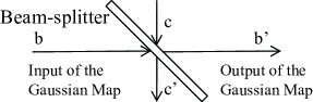
Figure 1: Gaussian map constructed by a beam-splitter. Here, we assume that the input mode $c$ is in the vacuum.

IV Efficient multimode-Gaussian QPT

Multimode Gaussian QPT has many important applications. For example, it applies to a complex linear optical circuit with BSs, squeezers, homodyne detections, linear losses, Gaussian noises, and so on. Consider now a Gaussian process acting on a $k$-mode input state (in modes $b_{1},b_{2},\cdots,b_{k}$), with outcome also a $k$-mode state. Even though other methods Lobino08 can also be extended to the multimode case, the number of input states required there increases exponentially with the number of modes $k$, because the number of ket-bra operators $|\{n_{i}\}\rangle\langle\{m_{i}\}|$ in Fock space increases exponentially with $k$. As shown below, the number of input states in our method increases polynomially.

A $k$-mode QPT can be tested with $k$-mode CSs, if the process is Gaussian. The main Eqs. (30)-(32) still hold after redefining the notations there. First, $\Gamma_{a},\;\Gamma_{b}$, $u$, $\alpha_{i}$, $d_{i}$, $Z_{a}$, and $Z_{b}$ are now $k$-mode vectors. For example,

$$|\alpha_{i}\rangle=|\alpha_{i1},\alpha_{i2},\cdots,\alpha_{ik}\rangle,$$

$$d_{i}=(d_{i1},d_{i2},\cdots,d_{ik}),\quad Z_{b}=(Z_{b1},Z_{b2},\cdots,Z_{bk}),$$

and so on. Following Eq. (15), $\mathcal{X}_{xy}$ is now a $k\!\times\!k$ matrix, for $\mathcal{X}=X$ or $Y$ with $x=a,b$; $y=a,b$. We still apply Eqs. (30)-(32) to calculate {$\Gamma_{b}$, $X_{ab},\;Y_{ab}$} and {$\Gamma_{a}$, $X_{aa}$, $Y_{aa}$}, respectively, but keep in mind that the matrices $K$, $J$ and symbols $d$, $c$ are now redefined. There are $(2k+1)k$ unknowns in ($\Gamma_{B},\;X_{ab},\;Y_{ab}$). We need $(2k+1)$ different CSs of $k$-mode to fix these unknowns. Now we have

$$K=\left(\begin{array}[]{ccc}1&\alpha_{1}^{*}&\alpha_{1}\\ 1&\alpha_{2}^{*}&\alpha_{2}\\ \vdots&\vdots&\vdots\\ 1&\alpha_{2k+1}^{*}&\alpha_{2k+1}\end{array}\right),$$ (44)

which is a $(2k+1)\times(2k+1)$ matrix, since each $\alpha_{i}$ here is a $k$-mode row vector. Moreover, $d$ is here a $(2k+1)\times k$ matrix as $d^{T}=\left(d_{1}^{T},\;d_{2}^{T},\cdots,d_{2k+1}^{T}\right)$, with $d_{i}=(d_{i1},d_{i2},\cdots,d_{ik})$. Similarly,

$$J=\left(\begin{array}[]{cccccc}1&\alpha_{1}^{*}&\alpha_{1}&{1\over 2}\alpha^{*2}_{1}&{1\over 2}\alpha^{2}_{1}&|\alpha_{1}|^{2}\\ 1&\alpha_{2}^{*}&\alpha_{2}&{1\over 2}\alpha^{*2}_{2}&{1\over 2}\alpha^{2}_{2}&|\alpha_{2}|^{2}\\ \vdots&\vdots&\vdots&\vdots&\vdots&\vdots\\ 1&\alpha_{N}^{*}&\alpha_{N}&{1\over 2}\alpha^{*2}_{N}&{1\over 2}\alpha^{2}_{N}&|\alpha_{N}|^{2}\end{array}\right),$$ (49)

which is now a $N\times N$ matrix, and $N=(k+1)(2k+1)$, since $\alpha_{i}^{2}$ and $|\alpha_{i}|^{2}$ here are row vectors of $\alpha^{2}_{i}=(E_{i1},\;E_{i2},\cdots,E_{ik})$ and $|\alpha_{i}|^{2}=(\tilde{E}_{i1},\;\tilde{E}_{i2},\cdots,\tilde{E}_{ik})$, and each element of $E_{im}$ (or $\tilde{E}_{im}$) is a vector with ($k-m+1$) modes (or $k$ modes), as

$$E_{im} = (\alpha_{im}^{2},\alpha_{im}\alpha_{i,m+1},\alpha_{im}\alpha_{i,m+2},\cdots,\alpha_{im}\alpha_{k},\alpha_{k}^{2}),$$

$$\tilde{E}_{im} = (\alpha_{im}\alpha^{*}_{i1},\alpha_{im}\alpha^{*}_{i2},\cdots,\alpha_{im}\alpha^{*}_{i,k-1},\alpha_{im}\alpha^{*}_{ik}).$$

Obviously, $c$ is a column vector with $N$ elements. Therefore we conclude with this:
Corollary: Any $k$-mode Gaussian QPT can be performed with $(k+1)(2k+1)$ different CSs of $k$-mode; or with $(2k+1)$ different CSs of $k$-mode if the process is trace preserving.

V Conclusions

In summary, we have presented explicit formulas for the tomography of quantum-optical Gaussian processes probed with only a few different coherent states. We have reduced the problem of Gaussian QPT to Gaussian QST, for which efficient methods are experimentally available Rehacek09 . We have extended our results to multimode Gaussian QPT and demonstrated that the number of test states required increases only polynomially with the number of modes.

- (1) J.F. Poyatos, J.I. Cirac, and P. Zoller, Phys. Rev. Lett. 78, 390 (1997).
- (2) I. L. Chuang and M. A. Nielsen, J. Mod. Opt. 44, 2455 (1997).
- (3) G.M. D’Ariano and P. Lo Presti, Phys. Rev. Lett. 86, 4195 (2001).
- (4) Quantum State Estimation, eds. M.G.A. Paris and J. Rehacek (Springer, Berlin, 2004).
- (5) M. Mohseni, A.T. Rezakhani, and D.A. Lidar, Phys. Rev. A 77, 032322 (2008).
- (6) J. Eisert and M. M. Wolf, in: Quantum Information with Continuous Variables of Atoms and Light, p. 23-42 (Imperial College Press, London, 2007).
- (7) D. W. Leung, J. Math. Phys. 44, 528 (2003).
- (8) J. B. Altepeter, D. Branning, E. Jeffrey, T. C. Wei, P. G. Kwiat, R. T. Thew, J. L. O Brien, M. A. Nielsen, and A. G. White, Phys. Rev. Lett. 90, 193601 (2003).
- (9) G.M. D’Ariano and P. Lo Presti, Phys. Rev. Lett. 91, 047902 (2003).
- (10) M. Mohseni and D. A. Lidar, Phys. Rev. Lett. 97, 170501 (2006); Phys. Rev. A 75, 062331 (2007).
- (11) Z.-W. Wang, Y.-S. Zhang, Y.-F. Huang, X.-F. Ren, and G.-C. Guo, Phys. Rev. A 75, 044304 (2007).
- (12) K. Lobino, D. Korystov, C. Kupchak, E. Figueroa, B.C. Sanders, and A.I. Lvovsky, Science 322, 563 (2008); S. Rahimi-Keshari, A. Scherer, A. Mann, A.T. Rezakhani, A.I. Lvovsky, and B.C. Sanders, New J. Phys. 13, 013006 (2011);
- (13) M. W. Mitchell, C. W. Ellenor, S. Schneider, and A. M. Steinberg, Phys. Rev. Lett. 91, 120402 (2003).
- (14) F. De Martini, A. Mazzei, M. Ricci, and G. M. D’Ariano, Phys. Rev. A 67, 062307 (2003).
- (15) J.L. O’Brien, G.J. Pryde, A. Gilchrist, D.F.V. James, N.K. Langford, T.C. Ralph, and A.G. White, Phys. Rev. Lett. 93, 080502 (2004).
- (16) Y. Nambu and K. Nakamura, Phys. Rev. Lett. 94, 010404 (2005).
- (17) N. K. Langford, T. J. Weinhold, R. Prevedel, K. J. Resch, A. Gilchrist, J. L. O Brien, G. J. Pryde, and A. G. White, Phys. Rev. Lett. 95, 210504 (2005).
- (18) N. Kiesel, C. Schmid, U. Weber, R. Ursin, and H. Weinfurter, Phys. Rev. Lett. 95, 210505 (2005).
- (19) X. S. Ma et al., Nature (London) 489, 269 (2012).
- (20) A. M. Childs, I. L. Chuang, and D. W. Leung, Phys. Rev. A 64, 012314 (2001).
- (21) N. Boulant, T. F. Havel, M. A. Pravia, and D. G. Cory, Phys. Rev. A 67, 042322 (2003).
- (22) Y.S. Weinstein, T.F. Havel, J. Emerson, N. Boulant, M. Saraceno, S. Lloyd, and D.G. Cory, J. Chem. Phys. 121, 6117 (2004).
- (23) Y.X. Liu, L.F. Wei, and F. Nori, Europhys. Lett. 67, 874 (2004); Phys. Rev. B72, 014547 (2005).
- (24) A.M. Zagoskin, S. Ashhab, J.R. Johansson, and F. Nori, Phys. Rev. Lett. 97, 077001 (2006).
- (25) M. Neeley, M. Ansmann, R. C. Bialczak, M. Hofheinz, N. Katz, E. Lucero, A. O’Connell, H. Wang, A. N. Cleland, and J. M. Martinis, Nat. Phys. 4, 523 (2008).
- (26) J.M. Chow et al., Phys. Rev. Lett. 102, 090502 (2009).
- (27) R. C. Bialczak et al., , Nat. Phys. 6, 409 (2010).
- (28) J. M. Chow et al., Phys. Rev. Lett. 109, 060501 (2012).
- (29) J.Q. You and F. Nori, Nature 474, 589 (2011); Phys. Today 58 (11), 42 (2005).
- (30) H. Kampermann and W. S. Veeman, J. Chem. Phys. 122, 214108 (2005).
- (31) M. Howard, J. Twamley, C. Wittmann, T. Gaebel, F. Jelezko, and J. Wrachtrup, New J. Phys. 8, 33 (2006).
- (32) D. Burgarth, K. Maruyama, and F. Nori, New J. Phys. 13, 013019 (2011).
- (33) M. Riebe, K. Kim, P. Schindler, T. Monz, P.O. Schmidt, T.K. Korber, W. Hansel, H. Haffner, C. F. Roos, and R. Blatt, Phys. Rev. Lett. 97, 220407 (2006).
- (34) T. Monz et al., Phys. Rev. Lett. 102, 040501 (2009).
- (35) S. H. Myrskog, J. K. Fox, M. W. Mitchell, and A. M. Steinberg, Phys. Rev. A 72, 013615 (2005).
- (36) A.S. Holevo and V. Giovannetti, Rep. Prog. Phys. 75, 046001 (2012).
- (37) A.S. Holevo, Probabilistic and Statistical Aspects of Quantum Theory (Springer, Berlin, 2011).
- (38) J. Rehacek, S. Olivares, D. Mogilevtsev, Z. Hradil, M. G. A. Paris, S. Fornaro, V. D’Auria, A. Porzio, and S. Solimeno, Phys. Rev. A 79, 032111 (2009).
- (39) J. Eisert, S. Scheel, and M.B. Plenio, Phys. Rev. Lett. 89, 137903 (2002); G. Giedke and J.I. Cirac, Phys. Rev. A 66, 032316 (2002).
- (40) W. H. Louisell, Quantum Statistical Properties of Radiation (Wiley, New York, 1973).
- (41) A. Jamiolkowski, Rep. Math. Phys. 3, 275 (1972).