Phase Equilibrium of Binary Mixtures in Mixed Dimensions

Abstract

We study the stability of a Bose-Fermi system loaded into an array of coupled one-dimensional (1D) “tubes”, where bosons and fermions experience different dimensions: Bosons are heavy and strongly localized in the 1D tubes, whereas fermions are light and can hop between the tubes. Using the ¹⁷⁴Yb-⁶Li system as a reference, we obtain the equilibrium phase diagram. We find that, for both attractive and repulsive interspecies interaction, the exact treatment of 1D bosons via the Bethe ansatz implies that the transitions between pure fermion and any phase with a finite density of bosons can only be first order and never continuous, resulting in phase separation in density space. In contrast, the order of the transition between the pure boson and the mixed phase can either be second or first order depending on whether fermions are allowed to hop between the tubes or they also are strictly confined in 1D. We discuss the implications of our findings for current experiments on ¹⁷⁴Yb-⁶Li mixtures as well as Fermi-Fermi mixtures of light and heavy atoms in a mixed dimensional optical lattice system.

I Introduction

The quest for lower temperatures in ultracold gases has lead to the development of many ingenious techniques to cool several atomic and molecular species. In particular, the explosion of activity concerning ultracold Fermi gases has become possible largely owing to the success of sympathetic cooling, which allows to efficiently cool fermions by mixing them with bosons Pethick and Smith (2002). At the same time, this procedure has stimulated the investigation, both experimental and theoretical, of Bose-Fermi mixtures. Here, the possibility of tuning the inter-species interaction strength using Feshbach resonances Courteille et al. (1998); Inouye et al. (1998); Bloch et al. (2008), has led to the exploration of many interesting phenomena such as collapse and phase separation Mølmer (1998); Viverit et al. (2000), as well as boson-mediated Cooper pairing Pethick and Smith (2002). Furthermore, Feshbach resonances can also be used to generate heteronuclear molecules, which can exhibit large electric dipole moments. This opens the interesting possibility of studying dipole-dipole interactions in quantum degenerate gases Wang et al. (2006); Wang (2007); Huang and Wang (2009); Santos et al. (2000); Micheli et al. (2006); Büchler et al. (2007); DeMille (2002).

Meanwhile, the advent of optical-lattice confinement Greiner et al. (2002); Bloch et al. (2008) has turned ultracold atomic gases into unique environments where to simulate and understand strongly correlated phenomena relevant to condensed matter systems. This has been made it possible, for example, by confining the atomic clouds in reduced dimensions, such as a one dimensional (1D) array of two-dimensional (2D) planes or a 2D array of 1D tubes. Whereas the former has enabled the study of interesting phenomena occurring in two-dimensions Posazhennikova (2006); Martiyanov et al. (2010), the latter has provided us with an amazingly tunable tool to explore the physics of interacting 1D quantum systems Moritz et al. (2005); Kinoshita (2004); Paredes et al. (2004); Cazalilla et al. (2011), of which it is much more difficult to find faithful realizations in a more conventional condensed matter context.

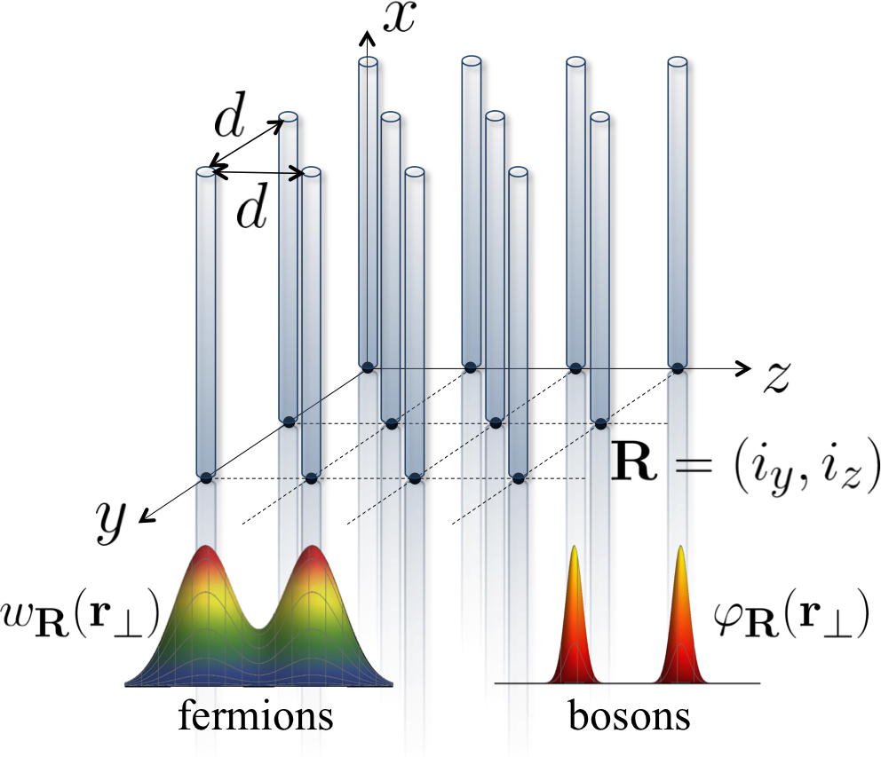
Figure 1: (Color online) Schematic representation of the system studied in this work, namely a mixed dimensionality Bose-Fermi system. The Bose-Fermi cloud is loaded in an anisotropic optical lattice that produces a two-dimensional $N_{y}\times N_{z}$ array of one-dimensional (1D) tubes of length $L$. The fermions are light enough to hop between the tubes whereas bosons, which are assumed to be much heavier, are confined in the 1D tubes. The bosonic and fermionic Wannier functions ($\varphi_{{\mathbf{R}}}({\mathbf{r}}_{\perp})$ and $w_{{\mathbf{R}}}({\mathbf{r}}_{\perp})$, respectively) are also displayed.

Optical lattice confinement has also allowed to envisage the realization of new types of quantum systems. One such example, analyzed in this work, is provided by mixtures of interacting particles in mixed-dimensional lattices. In recent years, these systems have attracted an increasing amount of theoretical attention Nishida and Tan (2008); Yang et al. (2011), and very recently they have been also experimentally realized Lamporesi et al. (2010); Minardi et al. (2011). Besides its intrinsic interest as a new category of quantum many-body systems, they may also offer advantages for reducing few-body losses and enhancing stability in strongly interacting regimes Marchetti et al. (2009).

In recent years, there has been a growing interest in understanding the properties of mixtures of ultracold Bose and Fermi gases. In particular, binary mixtures of bosons and spin-polarized fermions have been studied in three-dimensions (3D) Albus et al. (2003); Mølmer (1998); Viverit et al. (2000); Viverit and Giorgini (2002); Modugno et al. (2003); Günter et al. (2006), 2D Büchler and Blatter (2004) and 1D Das (2003); Lai and Yang (2011); Cazalilla and Ho (2003); Mathey et al. (2004); Imambekov and Demler (2006). Note that the 1D geometry has a special relevance because of the central role played by quantum fluctuations and the fact that there is neither broken continuous symmetry nor, consequently, off-diagonal long-range order. The equilibrium phase diagram of 1D Bose-Fermi mixtures has been considered by many authors Lai and Yang (2011); Das (2003); Cazalilla and Ho (2003); Mathey et al. (2004); Imambekov and Demler (2006), while the case of a Bose-Fermi system in an anisotropic optical lattices was studied by one of us in Ref. Marchetti et al. (2009).

In addition to dimensionality issues, the significant interest in studying the stability of binary mixtures comes also from the possibility of tuning the Bose-Fermi scattering length via the Feshbach resonance mechanism. Indeed, in the repulsive interaction regime, the spatial overlap between bosons and spin-polarized fermions is reduced, thus ensuring the stability of the system Zaccanti et al. (2006); Modugno (2007). When the repulsion is increased, the two components tend instead to phase separate, rather than uniformly mix: In the particular case of a 3D geometry, phase separation occurs either between a mixed phase and a purely fermionic phase or between two pure phases Viverit et al. (2000). In the regime where the interaction between bosons and fermions is attractive, a significant reduction of the interatomic distance can lead to a collapse of the mixture, because of three-body recombination processes Zirbel et al. (2008). As discussed later, the stability of the mixture towards a collapsed phase can be enhanced in one-dimensional geometries Marchetti et al. (2009).

In this article, we study the phase stability of a Bose-Fermi mixture embedded in a mixed-dimensional optical lattice of an array of one-dimensional tubes Jaksch et al. (1998); Stöferle et al. (2004) (see Fig. 1). The mixed-dimensionality comes from the fact that, while bosons are longitudinally confined along the tubes and strictly move in 1D, fermions are not constrained to 1D and are allowed to hop between tubes in the transverse directions. This assumption can be justified based on the fact that many realizations of Bose-Fermi mixtures consider bosonic species that are much heavier than the fermionic ones. We do also assume that, while bosons interact with each other, as well as with fermions, the fermionic component is polarized in a single hyperfine state and thus is non-interacting at very low temperatures.

As already mentioned, one motivation to study this geometry is that, by confining bosons in 1D, the mixture stability is enhanced Marchetti et al. (2009). Note that, even for purely bosonic gases, the spatial overlap between bosons has been experimentally shown to be strongly suppressed by the strong correlations emerging in 1D Kinoshita et al. (2005). In addition, mixed-dimensional systems allow to study interesting few-body Tan (2012) and many-body Yang et al. (2011); Malatsetxebarria et al. (2013) phenomena. We should stress that the results reported here are relevant to several experimental realizations. The simplest is, for example, a mixture of light fermions and heavy bosons. In particular, in order to make contact with ongoing and future experiments Hansen et al. (2013); Ivanov et al. (2011); Okano et al. (2010), we explicitly consider a mixture of ⁶Li (a light fermion) and ¹⁷³Yb (a heavy boson) atoms. An alternative realization could be given by an originally imbalanced mixture of fermions in two hyperfine states Chin et al. (2006): Bosons are then formed by associating fermions into Feshbach molecules Chin et al. (2006), leaving out from the pairing the spin polarized excess majority fermions. When the fermions belong to the same atomic species, the Feshbach molecules have twice the mass and twice the polarizability of the fermionic atoms. Therefore, it should be relatively easy to confine the bosons in 1D by loading them into a two-dimensional optical lattice. On the same lattice, the remaining majority fermions behave as the light component.

We find that, since bosons are confined to strictly 1D, they can undergo fermionization. This means that, as they mix with fermions, they form a Tonks-Girardeau gas whose energy per unit length grows as third power of the lineal density. As a result, we find that the nature of the transition from the pure Fermi gas to a mixture is always first order, implying phase separation in density space. Note that this is a very different result from the one obtained by assuming that bosons form a (quasi-)condensate, with the energy density growing as the square of the boson lineal density. The latter situation applies either to a high density Bose gas in 1D or to a gas of bosons that can hop in 3D. We also find that, in the mixed dimensionality lattice, the transition between pure boson and mixed phases is continuous, while it becomes first order when the fermions are also confined in 1D.

The rest of this article is organized as follows: In Sec. II we introduce the model for the Bose-Fermi mixture and discuss methods and approximations employed to derive the system phase diagram. In particular, in Sec. II.1, we explain how a mean-field approximation is applied solely to the boson-fermion interaction, whereas the boson-boson interaction is treated non-perturbatively using the Bethe ansatz in Sec. II.2. In Sec. III, we derive the phase diagram and interpret the origin of the discontinuous character of the transitions between the pure fermion and mixed phases in terms of an expansion of the free energy for small values of the boson density. We first describe the results obtained for the case of mixed dimensions in Sec. III.1 and later for the pure 1D limit in Sec. III.2. Finally, in Sec. IV, we present the main conclusions of our study and discuss the limitations of our approach, as well as some directions for future work. Some technical aspects of our derivations are provided in the appendices.

II Model

We consider a mixture of interacting bosonic ($B$) and single-component fermionic ($F$) atoms described by the following Hamiltonian (in $\hbar=1$ units):

$$\hat{H} =\hat{H}_{B}+\hat{H}_{F}+\hat{H}_{BF}\;,$$ (1)

$$\hat{H}_{B} =\int d{\mathbf{r}}\hat{\Psi}_{B}^{{\dagger}}\left[\displaystyle\frac{-\nabla^{2}}{2m_{B}}+V_{B}({\mathbf{r}})-\mu_{B}+\frac{g_{BB}}{2}\hat{\rho}_{B}\right]\hat{\Psi}^{\phantom{{\dagger}}}_{B}\;,$$

$$\hat{H}_{F} =\int d{\mathbf{r}}\hat{\Psi}_{F}^{{\dagger}}\left[\displaystyle\frac{-\nabla^{2}}{2m_{F}}+V_{F}({\mathbf{r}})-\mu_{F}\right]\hat{\Psi}^{\phantom{{\dagger}}}_{F}\;,$$

$$\hat{H}_{BF} =g_{BF}\int d{\mathbf{r}}\hat{\rho}_{B}(\mathbf{r})\hat{\rho}_{F}(\mathbf{r})\;,$$

where the density operators are $\hat{\rho}_{\alpha}({\mathbf{r}})=\hat{\Psi}^{{\dagger}}_{\alpha}({\mathbf{r}})\hat{\Psi}^{\phantom{{\dagger}}}_{\alpha}({\mathbf{r}})$, with $\alpha=B,F$. We have approximated all interaction potentials by contact interactions, which are parameterized by an $s$-wave scattering length $a_{\alpha\beta}$:

$$g_{\alpha\beta}=\displaystyle\frac{4\pi a_{\alpha\beta}}{m_{\alpha\beta}}\;,$$ (2)

being $m_{BB}=m_{B}$ and $m_{BF}=2m_{B}m_{F}/(m_{B}+m_{F})$. For thermodynamic stability reasons, the bosons are assumed to repel each other (i.e., $a_{BB}>0$). The value of $a_{BB}$ can be tuned by, e.g., controlling the strength of the transverse confinement Olshanii (1998). The sign of the Bose-Fermi interaction strength is determined by $a_{BF}$, which can be controlled independently from $a_{BB}$ by resorting to an inter-species Feshbach resonance. Below we consider both the repulsive ($a_{BF}>0$) as well as the attractive ($a_{BF}<0$) case. At ultracold temperatures, interactions between identical fermions can be safely neglected.

The Bose-Fermi mixture is loaded into an anisotropic optical lattice formed by a 2D $N_{y}\times N_{z}$ square array of 1D “tubes” of length $L$ directed along the $x$-direction and equally spaced by a distance $d$ (see Fig. 1). This can be described by an optical potential of the form $V_{\alpha}({\mathbf{r}}_{\perp})=V^{\alpha}_{0}[\sin^{2}(\pi y/d)+\sin^{2}(\pi z/d)]$, where ${\mathbf{r}}_{\perp}=(y,z)$. The strength of the optical potential $V^{B}_{0}$ ($V^{F}_{0}$) is determined by both the laser intensity and the boson (fermion) atomic polarizability, allowing the possibility of mixed dimensionality for the mixture. In particular, we assume that the bosons are tightly confined in 1D tubes and thus move strictly in 1D, while fermions can hop between the tubes. We will derive the thermodynamic phase diagram for this geometry, thus neglecting the harmonic confinement. By making use of the local density approximation, information about the experimentally relevant trapped case can be extracted from the homogeneous phase diagram plotted in chemical potential space.

Because the bosons in the mixture are assumed to be more massive than fermions and/or to experience a more confining lattice potential $V_{B}({\mathbf{r}}_{\perp})$, they are tightly confined along the “tubes”, a configuration often refereed to as a two-dimensional optical lattice Greiner et al. (2002); Kinoshita (2004); Stöferle et al. (2004); Moritz et al. (2003); Cazalilla et al. (2006, 2011). Thus, the field operator $\hat{\Psi}^{\phantom{{\dagger}}}_{B}({\mathbf{r}})$ can be expressed in terms of Wannier functions $\varphi^{\phantom{*}}_{{\mathbf{R}}}({\mathbf{r}}_{\perp})$ localized at the tube site ${\mathbf{R}}=(i_{y},i_{z})d$ (see, e.g., Bloch et al. (2008) and references therein) and the tube boson operator $\hat{\Psi}^{\phantom{{\dagger}}}_{B{\mathbf{R}}}(x)$:

$$\hat{\Psi}^{\phantom{{\dagger}}}_{B}({\mathbf{r}})=\sum_{{\mathbf{R}}}\varphi^{\phantom{*}}_{{\mathbf{R}}}({\mathbf{r}}_{\perp})\hat{\Psi}^{\phantom{{\dagger}}}_{B{\mathbf{R}}}(x)\;.$$ (3)

The Wannier functions form an orthonormal basis. By neglecting the interactions between tubes with $\mathbf{R}\neq\mathbf{R}^{\prime}$, we can rewrite the bosonic Hamiltonian $\hat{H}_{B}$ in (1) as a sum of decoupled 1D Hamiltonians,

$$\hat{H}_{B}=\sum_{\mathbf{R}}\int dx\hat{\Psi}_{B{\mathbf{R}}}^{\dagger}(x)\left[\displaystyle\frac{-\partial_{x}^{2}}{2m_{B}}-\mu_{B}^{1D}\right.\\ \left.+\frac{g^{1D}_{BB}}{2}\hat{\rho}_{B{\mathbf{R}}}(x)\right]\hat{\Psi}^{\phantom{{\dagger}}}_{B{\mathbf{R}}}(x)\;,$$ (4)

where $\hat{\rho}_{B{\mathbf{R}}}(x)=\hat{\Psi}_{B{\mathbf{R}}}^{{\dagger}}(x)\hat{\Psi}^{\phantom{{\dagger}}}_{B{\mathbf{R}}}(x)$ is the single-tube boson density operator, $g^{1D}_{BB}$ is the one-dimensional boson coupling, which, for weak boson-boson interaction, takes the form:

$$g_{BB}^{1D}=g_{BB}\int d\mathbf{r}_{\perp}|\varphi^{\phantom{*}}_{{\mathbf{R}}}(\mathbf{r}_{\perp})|^{4}\;,$$ (5)

and $\mu_{B}^{1D}$ is the 1D boson chemical potential:

$$\mu_{B}^{1D}=\int d{\mathbf{r}}_{\perp}\varphi_{{\mathbf{R}}}^{*}({\mathbf{r}}_{\perp})\left[\displaystyle\frac{\nabla^{2}_{\perp}}{2m_{B}}-V_{B}({\mathbf{r}}_{\perp})+\mu_{B}\right]\varphi^{\phantom{*}}_{{\mathbf{R}}}({\mathbf{r}}_{\perp})\;.$$

Note that, as we will see later, for strong boson-boson interactions, the expression of the 1D boson coupling $g^{1D}_{BB}$ is instead given by Eq. (28) Olshanii (1998) rather than Eq. (5).

In contrast, we assume the fermions to be more weakly confined than bosons along each tube due to their smaller mass and/or a weaker optical potential. Yet, the lattice confinement is strong enough so that the description of the Fermi field in terms on the lowest Bloch band $\phi_{{\mathbf{k}}_{\perp}}({\mathbf{r}}_{\perp})$ is accurate and we can expand:

$$\hat{\Psi}^{\phantom{{\dagger}}}_{F}({\mathbf{r}})=\displaystyle\frac{1}{\sqrt{L}}\sum_{{\mathbf{k}}}e^{ik_{x}x}\phi_{{\mathbf{k}}_{\perp}}({\mathbf{r}}_{\perp})\hat{f}^{\phantom{{\dagger}}}_{{\mathbf{k}}}\;,$$ (6)

where ${\mathbf{k}}=(k_{x},{\mathbf{k}}_{\perp})$. Here, whereas the motion along the $x$ direction is free, the motion in the transverse directions ${\mathbf{r}}_{\perp}=(y,z)$ is described by $\phi_{{\mathbf{k}}_{\perp}}({\mathbf{r}}_{\perp})$, which is a Bloch wavefunction belonging to the lowest Bloch band characterized by a crystal momentum ${\mathbf{k}}_{\perp}$. Projecting the fermion Hamiltonian onto this band yields:

$$\hat{H}_{F}=\sum_{{\mathbf{k}}}\left[\varepsilon({\mathbf{k}})-\mu_{F}\right]\hat{f}^{{\dagger}}_{{\mathbf{k}}}\hat{f}^{\phantom{{\dagger}}}_{{\mathbf{k}}}\;,$$ (7)

where the Fermion dispersion reads as:

$$\varepsilon({\mathbf{k}}) =\displaystyle\frac{k^{2}_{x}}{2m_{F}}+\epsilon({\mathbf{k}}_{\perp})\;$$ (8)

$$\epsilon({\mathbf{k}}_{\perp}) =2t\left[2-\cos(k_{y}d)-\cos(k_{z}d)\right]\;.$$ (9)

Thus, summarizing, in the geometry studied here, the bosons are tightly confined to move in 1D, whereas the fermions can hop between the tubes, although the optical lattice potential does affect their dispersion relation. Under these conditions, it is known Cazalilla et al. (2011) that, at low temperatures, the bosonic atoms loose their individuality and the low-energy long-wavelength excitations are 1D phonons. For arbitrary values of $g^{1D}_{BB}>0$, the ground state properties of such an interacting bosonic gas are exactly described by the Bethe ansatz solution obtained by Lieb and Liniger Lieb and Liniger (1963). The lack of individuality and the highly correlated behavior brought about by the 1D confinement calls for a treatment of the problem that treats the boson-boson interactions in a non-perturbative way. Since a mean-field approximation fails to capture the fundamental bosonic correlations in 1D, we apply it only to the interactions between the fermions and the bosons, as we explain in what follows.

II.1 Bose-Fermi interaction: mean-field

In order to render the above model tractable, we apply a mean-field approximation to the Bose-Fermi interaction term. We do this in such a way that the different 1D tubes become decoupled at the expense of introducing self-consistent shifts of both the boson and fermion chemical potentials. To this end, we first observe that the tight confinement of the bosons in 1D allows us to neglect the overlap between Wannier functions localized at different 1D tubes (see Fig. 1) and thus we can approximate the density operator of the bosons as

$$\hat{\rho}_{B}({\mathbf{r}})\simeq\sum_{{\mathbf{R}}}|\varphi^{\phantom{*}}_{{\mathbf{R}}}({\mathbf{r}}_{\perp})|^{2}\hat{\rho}_{B{\mathbf{R}}}(x)\;.$$

In this limit, the Bose-Fermi interaction term $\hat{H}_{BF}$ of the Hamiltonian (1) can be written as

$$\hat{H}_{BF}\simeq g_{BF}\sum_{{\mathbf{R}}}\int dx\hat{\rho}_{B{\mathbf{R}}}(x)\hat{\rho}_{F{\mathbf{R}}}(x)\;,$$ (10)

where $\hat{\rho}_{F{\mathbf{R}}}(x)$ is a projection of the 3D Fermi density operator $\hat{\rho}_{F}({\mathbf{r}})$ on the ${\mathbf{R}}$-th tube:

$$\hat{\rho}_{F{\mathbf{R}}}(x)=\int d{\mathbf{r}}_{\perp}|\varphi^{\phantom{*}}_{{\mathbf{R}}}({\mathbf{r}}_{\perp})|^{2}\hat{\rho}_{F}({\mathbf{r}})\;.$$ (11)

We note that this approximation does not decouple the different tubes yet because, even if bosons cannot hop from one tube to another, the interaction between bosons belonging to different tubes is mediated by the hopping fermions, i.e., the operator $\hat{\rho}_{F{\mathbf{R}}}(x)$. However, if we rely on a mean-field approximation to replace the operator $\hat{\rho}_{F{\mathbf{R}}}(x)$ by its expectation value (which, as shown in detail in App. A, is a constant), the different tubes become decoupled, which allows for a solution of the model introduced above. We emphasize again that this kind of mean-field approximation is different from the standard treatment (for example employed in Ref. Marchetti et al. (2009)), where also the boson density in the boson-boson interaction term is replaced with its expectation value. Instead, here the boson interaction is treated non-perturbatively using the Bethe ansatz, emphasizing that the fundamental entities subject to the mean-field interaction are the 1D tubes and not the bosons themselves.

Thus, in Eq. (10), we write the density operators $\hat{\rho}_{\alpha{\mathbf{R}}}(x)$ as their quantum averages plus fluctuations, i.e. $\hat{\rho}_{\alpha{\mathbf{R}}}(x)=\langle\hat{\rho}_{\alpha{\mathbf{R}}}(x)\rangle+\delta\hat{\rho}_{\alpha{\mathbf{R}}}(x)$. Hence, the mean-field approximation is obtained by substituting these expressions into Eq. (10) and by neglecting the second order terms in the fluctuations, which leads to:

$$\hat{H}_{BF}\simeq H^{mf}_{BF}=g_{BF}\sum_{{\mathbf{R}}}\int dx\left[-\langle\hat{\rho}_{B{\mathbf{R}}}(x)\rangle\langle\hat{\rho}_{F{\mathbf{R}}}(x)\rangle\right.\\ \left.+\hat{\rho}_{B{\mathbf{R}}}(x)\langle\hat{\rho}_{F{\mathbf{R}}}(x)\rangle+\langle\hat{\rho}_{B{\mathbf{R}}}(x)\rangle\hat{\rho}_{F{\mathbf{R}}}(x)\right]\;.$$ (12)

In absence of harmonic confinement along the tubes, translational invariance along the $x$-direction requires that the averages

$$\langle\hat{\rho}_{B{\mathbf{R}}}(x)\rangle =\rho^{0}_{B} \langle\hat{\rho}_{F{\mathbf{R}}}(x)\rangle =A\>\rho^{0}_{F}$$ (13)

are constants independent on the tube index ${\mathbf{R}}$. Here, the constant

$$A\simeq N\int d{\mathbf{r}}_{\perp}|\varphi^{\phantom{*}}_{{\mathbf{R}}}({\mathbf{r}}_{\perp})|^{2}|\phi_{{\mathbf{k}}_{\perp}}({\mathbf{r}}_{\perp})|^{2}\;,$$ (14)

it is obtained in the limit where the transverse confinement for the bosons is tight (see App. A for the details of the derivation). Also, we have introduced the following lineal densities:

$$\rho_{\alpha}^{0}=\displaystyle\frac{N_{\alpha}}{NL}\;,$$ (15)

where $N=N_{y}N_{z}$ is the total number of 1D tubes. Thus, within this mean-field approximation, the system Hamiltonian (1) can be written as

$$\hat{H}\simeq\hat{H}^{mf}=\hat{H}_{B}^{mf}+\hat{H}_{F}^{mf}-\sum_{{\mathbf{R}}}g_{BF}A\rho^{0}_{B}\rho^{0}_{F}\;,$$ (16)

where $\hat{H}_{B}^{mf}$ is defined as the bosonic Hamiltonian from Eq. (4) with the chemical potential shifted as $\mu_{B}^{1D}\to\mu_{B}^{1D}-g_{BF}A\rho^{0}_{F}$:

$$\hat{H}_{B}^{mf}=\sum_{{\mathbf{R}}}\int dx\hat{\Psi}_{B{\mathbf{R}}}^{\dagger}(x)\left[\displaystyle\frac{-\partial_{x}^{2}}{2m_{B}}-\mu_{B}^{1D}+g_{BF}A\rho^{0}_{F}\right.\\ \left.+\frac{g^{1D}_{BB}}{2}\hat{\rho}_{B{\mathbf{R}}}(x)\right]\hat{\Psi}^{\phantom{{\dagger}}}_{B{\mathbf{R}}}(x)\;,$$ (17)

and $\hat{H}_{F}^{mf}$ is the fermion Hamiltonian from Eq. (7) with a chemical potential shifted as $\mu_{F}\to\mu_{F}-g_{BF}A\rho^{0}_{B}$:

$$\hat{H}_{F}^{mf}=\sum_{{\mathbf{k}}}\left[\varepsilon({\mathbf{k}})-\mu_{F}+g_{BF}A\rho^{0}_{B}\right]\hat{f}^{{\dagger}}_{{\mathbf{k}}}\hat{f}^{\phantom{{\dagger}}}_{{\mathbf{k}}}$$ (18)

We would like to stress that we are not applying a mean-field approximation to the boson-boson interaction term $\hat{\rho}^{2}_{B{\mathbf{R}}}(x)$. On the contrary, as shown in the next section, we shall treat this term exactly using the Bethe ansatz solution of Eq. (17) due to Lieb and Liniger Lieb and Liniger (1963).

II.2 Zero-temperature free energy

Starting from the mean-field Hamiltonian defined by equations (16), (17), and (18), we can evaluate the grand-canonical free energy density at zero temperature. Note that, by virtue of the mean-field approximation and the translational invariance, the bosonic $\hat{\Psi}^{\phantom{{\dagger}}}_{B{\mathbf{R}}}$ and fermionic $\hat{f}^{\phantom{{\dagger}}}_{{\mathbf{k}}}$ field operators in Eq. (16) have become decoupled and therefore we can separate the bosonic and a fermionic contributions to the free energy potential $f=f(\mu_{B}^{1D},\mu_{F},\rho_{B}^{0})$, which can be written as:

$$f=\frac{(\rho_{B}^{0})^{3}}{2m_{B}}e(\gamma)-\mu_{B}^{1D}\rho_{B}^{0}-\displaystyle\frac{1}{N}\sum_{{\mathbf{k}}_{\perp}\in BZ}\displaystyle\frac{k_{Fx}^{3}({\mathbf{k}}_{\perp})}{3\pi m_{F}}\;,$$ (19)

where $BZ$ stands for the 2D Brillouin zone, i.e., the region of ${\mathbf{k}}_{\perp}$-space where $|k_{y,z}|\leq\pi/d$. In evaluating this expression, we have relied upon the Bethe ansatz solution Lieb and Liniger (1963); Cazalilla et al. (2011) of the interacting 1D boson Hamiltonian, $\hat{H}_{B}^{mf}$ (17). It is worth noting that the constant term $g_{BF}A\rho^{0}_{B}\rho^{0}_{F}$ in Eq. (16) cancels exactly the mean-field shift of the bosonic chemical potential, $\mu_{B}^{1D}\to\mu_{B}^{1D}-g_{BF}A\rho^{0}_{F}$, in Eq. (17).

In Eq. (19), the dimensionless function $e(\gamma)$, where $\gamma=m_{B}g_{BB}^{1D}/\rho_{B}^{0}$, is determined by numerically solving the following system of coupled integral equations:

$$e(\gamma) =\frac{\gamma^{3}}{l^{3}}\int_{-1}^{1}duu^{2}g(u)\;,$$ (20)

$$2\pi g(u) =1+2l\int_{-1}^{1}du^{\prime}\frac{g(u^{\prime})}{(u-u^{\prime})^{2}+l^{2}}\;,$$ (21)

where $l=\gamma\int_{-1}^{1}du\>g(u)$. The fermionic contribution to the free energy can be expressed as an integral over the transverse momentum, which leads to the last term in Eq. (19), where we have defined:

$$k_{Fx}({\mathbf{k}}_{\perp})=\text{Re}\sqrt{2m_{F}\left[\mu_{F}-g_{BF}A\rho_{B}^{0}-\epsilon({\mathbf{k}}_{\perp})\right]}\;.$$

Finally, the thermodynamic grand-canonical free energy density is obtained by finding the global minimum of the potential $f(\mu_{B}^{1D},\mu_{F},\rho_{B}^{0})$ with respect to the boson density $\rho_{B}^{0}$:

$$\Omega(\mu_{B}^{1D},\mu_{F})=\min_{\rho_{B}^{0}=n_{B}}f(\mu_{B}^{1D},\mu_{F},\rho^{0}_{B})\;,$$ (22)

where $n_{B}$ denotes the equilibrium lineal boson density. Note that, since Bose-Einstein condensation is not allowed in 1D interacting boson systems Cazalilla et al. (2011), the boson density cannot be regarded as the condensate density, i.e., the square of the condensate order parameter. In addition, the equilibrium 1D fermionic density can be evaluated from

$$n_{F}=\displaystyle\frac{1}{N}\sum_{{\mathbf{k}}_{\perp}\in BZ}\displaystyle\frac{k_{Fx}({\mathbf{k}}_{\perp})}{\pi}\;.$$ (23)

As explained in the next section, we can thus now evaluate the system equilibrium phase diagram either in chemical potential or in density space.

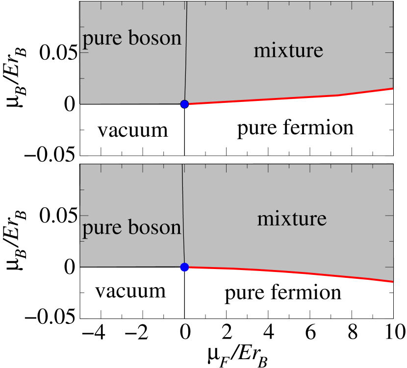
Figure 2: (Color online) Zero temperature phase diagrams for a repulsive ($a_{BF}>0$, top panel) and attractive $a_{BF}<0$ (bottom panel) Bose-Fermi mixture with fixed dimensionless hopping amplitude $\tilde{t}=37.8$ and fixed interaction parameter $\zeta=0.23$ (the parameters of this calculation correspond to a ¹⁷⁴Yb-⁶Li system, see main text). The diagrams are plotted vs. the boson $\mu_{B}^{1D}/Er_{B}$ and fermion $\mu_{F}/Er_{B}$ chemical potentials, where $Er_{B}$ is the boson recoil energy — note that $\mu^{1D}_{B}/Er_{B}\ll 1$, thus ensuring that the bosons remain confined to 1D throughout. The thin solid black lines correspond to 2nd order (i.e. continuous) phase transitions between either the vacuum and the pure boson/fermion phases or between the pure boson and the homogeneous mixed phase. The thick solid (red) line corresponds to a first order transition between the pure fermion and the mixed phase. Second and first order lines meet at at the tricritical point at $\mu_{F}=\mu_{B}=0$ (filled blue circle). The region with finite boson density is the light gray shaded region. In both cases phase separation can only occur between a mixed and pure fermion phases.

III Phase diagram

In this section, we obtain the phase diagram of the mixed-dimensionality system by minimizing the free energy introduced above in Eq. (19) with respect to the boson density $\rho_{B}^{0}$ for fixed $\mu_{B}^{1D}$ and $\mu_{F}$. The free energy $f(\mu_{B}^{1D},\mu_{F},\rho^{0}_{B})$ also depends on several other parameters, such as $g_{BF}$, $g_{BB}^{1D}$, and $t$, as well as the particle masses $m_{B},m_{F}$. Thus, it is convenient to simplify the description of the system by considering the following minimal set of four independent dimensionless parameters:

$$\tilde{\mu}_{B}^{1D} =\frac{2m_{B}\mu_{B}^{1D}}{c^{2}} \tilde{\mu}_{F} =\frac{2m_{F}^{1/3}m_{B}^{2/3}\mu_{F}}{c^{2}}\;$$ (24)

$$\tilde{t} =\frac{2m_{F}^{1/3}m_{B}^{2/3}t}{c^{2}} \zeta =\frac{c}{2m_{B}g_{BB}^{1D}}\;,$$ (25)

where $c=2Am_{F}^{1/3}m_{B}^{2/3}|g_{BF}|$. Thus, the dimensionless interaction parameter $\gamma$ can we rewritten as $\gamma=(2\zeta\tilde{\rho}_{B}^{0})^{-1}$, with the dimensionless boson density given by $\tilde{\rho}_{B}^{0}=\rho^{0}_{B}/c$. In terms of the above dimensionless quantities, the free energy takes the form:

$$\tilde{f}=(\tilde{\rho}_{B}^{0})^{3}e(\gamma)-\tilde{\mu}_{B}^{1D}\tilde{\rho}_{B}^{0}-\displaystyle\frac{1}{N}\sum_{{\mathbf{k}}_{\perp}\in BZ}\displaystyle\frac{\tilde{k}_{Fx}^{3}({\mathbf{k}}_{\perp})}{3\pi m_{F}}\;,$$ (26)

where $\tilde{k}_{Fx}({\mathbf{k}}_{\perp})=\text{Re}\sqrt{\tilde{\mu}_{F}-\text{sign}(g_{BF})\tilde{\rho}_{B}^{0}-\tilde{\epsilon}({\mathbf{k}}_{\perp})}$ and $\tilde{\epsilon}({\mathbf{k}}_{\perp})=2\tilde{t}[2-\cos(k_{y}d)-\cos(k_{z}d)]$.

III.1 Mixed dimensions

We explicitly consider here the case of mixed dimensions, while later in Sec. III.2, we will derive the phase diagram for the case of pure 1D. We have numerically minimized $\tilde{f}$ by fixing the value of the dimensionless interaction parameter, $\zeta$, and hopping amplitude, $\tilde{t}$. In order to make contact with ongoing as well as future experiments Hansen et al. (2013); Ivanov et al. (2011); Okano et al. (2010), we consider the specific case of a Bose-Fermi system consisting of a light fermionic species such as ⁶Li and a heavy bosonic species like ¹⁷⁴Yb. When this system is loaded in a sufficiently deep 2D optical lattice, the large boson to fermion mass ratio ($m_{B}/m_{F}\simeq 29$) is enough to suppress the hopping between tubes of bosons, while allowing fermions to hop between the tubes. This makes it possible to realize our initial assumption of mixed dimensionality for the system. Indeed, in the limit of a deep lattice, the fermion hopping amplitude in the tight-binding approximation of Eq. (7) can be expressed in terms of the optical potential strength $V^{F}_{0}$ and the Fermi recoil energy $Er_{F}$, where $Er_{\alpha}=2\pi^{2}/(m_{\alpha}\lambda^{2})$ and $\lambda=2d$ is the wavelength of the laser generating the optical lattice potential Bloch et al. (2008):

$$t\simeq\frac{4Er_{F}}{\sqrt{\pi}}\left(\displaystyle\frac{V_{0}^{F}}{Er_{F}}\right)^{3/4}e^{-2\sqrt{V_{0}^{F}/Er_{F}}}\;.$$ (27)

For a laser wavelength $\lambda=1064$ nm, the deep lattice condition is achieved by making $V^{B}_{0}\simeq 40Er_{B}$ (for this system $V^{F}_{0}\simeq 2V^{B}_{0}$ Hansen et al. (2013); Takahashi (2013)). Furthermore, the boson-boson scattering  (2) length has been experimentally estimated to be $a_{BB}=104.9~{}a_{0}$ Kitagawa et al. (2008) (where $a_{0}$ is the Bohr radius). The 1D interaction strength $g_{BB}^{1D}$ can be obtained from Olshanii (1998):

$$\frac{1}{g_{BB}^{1D}}=\frac{m_{B}\ell_{B}}{2}\left(\frac{\ell_{B}}{a_{BB}}-C\right)\;,$$ (28)

where $C\simeq 1.0326$ and $\ell_{B}=67.34$ nm . For these parameters, $\ell_{F}=131.40$ nm, and therefore, using Eq. (34), $A=1.46017\times 10^{13}~{}\mathrm{m^{-2}}$. Finally, we set $|a_{BF}|=13~{}a_{0}$ Hansen et al. (2013), and allow for both positive and negative signs for $a_{BF}$, i.e. for the Bose-Fermi interactions to be repulsive or attractive. Using these values, the dimensionless interaction and hoping parameters are $\tilde{t}=37.8$ and $\zeta=0.23$.

The phase diagrams for repulsive ($a_{BF}>0$) and attractive ($a_{BF}<0$) Bose-Fermi interactions are shown in Fig. 2 as a function of the boson and fermion chemical potentials. In both cases, a qualitatively similar structure emerges: The transition between the pure fermion and the phase where boson and fermions form a homogeneous mixture (mixed phase) is first order (thick solid red line). For the particular values of parameters chosen in Fig. 2 to describe the ¹⁷⁴Yb-⁶Li mixture, we numerically find that the transition is weakly first order close to the origin $(\mu_{F},\mu_{B}^{1D})=(0,0)$, i.e., the chemical potential values for which the slope of the free energy at $\rho^{0}_{B}=0$ changes sign are very close to the values of chemical potentials at the transition. On the other hand, the transition between the pure boson and the mixed phases (thin solid black line) is second order, i.e. continuous. This transition coincides with the locus of points where the system first develops a Fermi surface, i.e., $\tilde{\mu}_{F}-\text{sign}(g_{BF})\tilde{\rho}_{B}^{0}=0$, and therefore $\mu_{F}>0$ ($\mu_{F}<0$) for repulsive (attractive) interactions. In App. B, we carry on an expansion for small fermion density which allows to establish the nature of the phase transitions where the number of Fermi surfaces changes from zero to one. There, we argue that this transition is continuous because of the scaling that the Fermi kinetic energy has with the fermion density in 3D, while it would be first order if the fermion would also move in strictly 1D like the bosons. This result is also in agreement with the conclusion reached by Viverit et al. for Bose-Fermi mixtures in 3D Viverit and Giorgini (2002), where they show that phase separation between a mixed phase and a pure boson phase cannot be realized in 3D.

Finally, the transitions between the vacuum, corresponding to zero density of both fermions and bosons, and either the pure boson or fermion phases (thin solid black lines in Fig. 2) are continuous, as they correspond to the filling of a band Sachdev (2010). Therefore, the first order line separating the pure fermion and mixed phases terminates at the origin $(\mu_{F},\mu_{B}^{1D})=(0,0)$ in a tricritical point (filled blue circle), where the first order transition becomes second order.

A first order transition in the phase diagram in chemical potential space implies that the system exhibits phase separation in density space, where, rather than fixing the chemical potentials $\mu_{F}$ and $\mu_{B}^{1D}$, one fixes the boson $n_{B}$ and fermion $n_{F}$ densities (see Fig. 3). We obtain therefore that, for finite inter-tube hopping $t$, phase separation is only possible between pure fermion and mixed phases (dot-dashed black lines in Fig. 3). In Sec. III.2, we will see that this fact is related to the dimensionality where fermions move and that the situation drastically changes for strictly 1D, e.g., when the hopping $t$ for fermions is reduced to zero. Note also that, for attractive interactions, in contrast to a 3D Bose-Fermi mixtures in the absence of the lattice Viverit et al. (2000); Pethick and Smith (2002), the system is found to exhibit phase separation rather than collapse. This result was also obtained in Ref. Marchetti et al. (2009), by treating the boson-boson interactions within the mean-field approximation. However, different from that work, the non-perturbative treatment of the boson interactions employed here, yields a first order transition between the pure fermion and mixed phases.

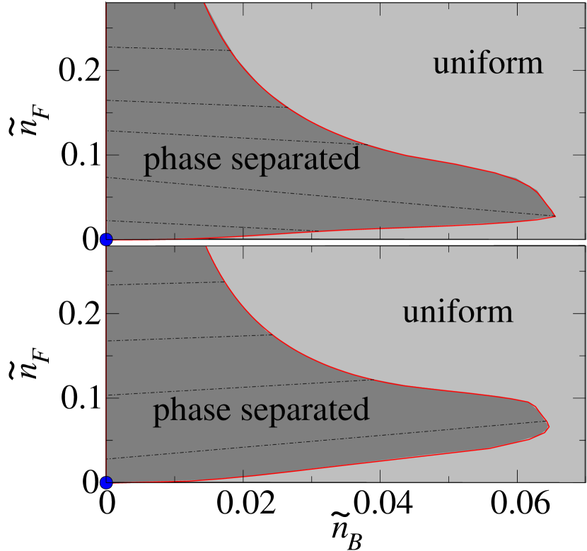
Figure 3: (Color online) Phase diagrams in the density plane $(\tilde{n}_{B},\tilde{n}_{F})$. In order to obtain a more accurate estimate of the phase boundaries, we have used the parameters $\tilde{t}=0.023$ and $\zeta=0.27$. The corresponding phase diagrams in the chemical potential plane (not shown for brevity) display the same features and phase topology as the diagrams shown Fig. 2, which are computed for the experimentally relevant a ¹⁷⁴Yb-⁶Li system, but for which the phase boundary in the density plane proved much harder to determine numerically. The top panel corresponds to a repulsive Bose-Fermi interactions, whereas in the bottom corresponds to attractive interactions. In both cases, the system can either be in a uniform mixed phase (lightly gray shaded region) or, by undergoing a first order transition, it can be in a phase separated state (dark gray shaded region), where a pure fermion and mixed phase coexist. The dot-dashed lines connect points on the first order boundary with the same values of the chemical potentials.

The absence of a continuous phase transition between the pure fermion and any phase with a finite density of bosons can be qualitatively understood by making an analogy with the Landau theory of phase transitions and considering the series expansion of the free energy $\tilde{f}$ in (26) for small values of the boson density $\tilde{\rho}_{B}^{0}$. In this limit, for fixed $\zeta^{-1}\propto g^{1D}_{BB}$, we have that $\gamma=(2\zeta\tilde{\rho}_{B}^{0})^{-1}\gg 1$, and therefore the Bose gas is essentially fermionized and close to a Tonks gas. Thus, we can use the following asymptotic formula for the boson energy Lieb and Liniger (1963); Cazalilla (2003):

$$e(\gamma)\operatorname*{\simeq}_{\gamma\to\infty}e_{TG}\left[1-\frac{4}{\gamma}+O(\gamma^{-2})\right]\;,$$

where $e_{TG}=\pi^{2}/3$. Note that this expression implies that the boson contribution to the free energy grows as $(\rho^{0}_{B})^{3}$. This yields the following series expansion for the free energy at small boson density:

$$\tilde{f}=\tilde{f}_{0}+\tilde{f}_{2}\tilde{\rho}_{B}^{0}+\tilde{f}_{2}(\tilde{\rho}_{B}^{0})^{2}+\tilde{f}_{6}(\tilde{\rho}_{B}^{0})^{3}+\cdots\;,$$ (29)

where the coefficients of the expansion are given by:

$$\tilde{f}_{2} =\text{sign}(g_{BF})C_{1}-\tilde{\mu}_{B}^{1D}\;,$$

$$\tilde{f}_{4} =-C_{-1}/4\;,$$

$$\tilde{f}_{6} =e_{TG}-\text{sign}(g_{BF})C_{-3}/24\;,$$

and where $C_{n}=\frac{1}{\pi N}\sum_{{\mathbf{k}}_{\perp}\in BZ}\text{Re}\left[\sqrt{\tilde{\mu}_{F}-\tilde{\epsilon}({\mathbf{k}}_{\perp})}\right]^{n}\geq 0$ ($|n|$ is odd). In addition, note that $C_{n}=0$ if $\mu_{F}=0$. Thus, for $\mu_{F}>0$, a continuous phase transition cannot take place because the coefficient $\tilde{f}_{4}$ of the above expansion is always negative meaning that for $\tilde{f}_{2}>0$ the free energy must eventually decrease away from the origin where $\tilde{\rho}_{B}^{0}=0$ before it can rise again ($\tilde{f}_{6}>0$ is assumed, for stability). Thus, the free energy develops a local minimum for $\tilde{\rho}_{B}^{0}\neq 0$, which eventually can be tuned to be degenerate with the local minimum at $\rho^{0}_{B}=0$. It is worth comparing this situation with the result of the mean-field treatment of bosons interactions carried out by one of us in Ref. Marchetti et al. (2009), where it was found that $\tilde{f}_{4}=(2-\zeta C_{-1})/(4\zeta)$, thus allowing both second and first order phase transitions to occur for $\mu_{F}>0$ by tuning $\tilde{f}_{2}=0$ and $\tilde{f}_{4}=0$.

In addition, we can use the above expressions to understand the emergence of a tricritical point, which corresponds to the conditions $\tilde{f}_{2}=0=\tilde{f}_{4}$ while $\tilde{f}_{6}>0$ for stability. Since $C_{n}=0$ only for $\mu_{F}=0$, we can conclude that a stable tricritical point can only exist at the origin of the chemical potential plane, i.e. for $(\mu_{F},\mu_{B}^{1D})=(0,0)$. Close to the tricritical point, the shape of the first order line can also obtained analytically using the conditions $\tilde{f}_{2}>0$ and $\tilde{f}_{4}=-2\sqrt{\tilde{f}_{2}\tilde{f}_{6}}$. Note that for the choice of parameters done to describe the ¹⁷⁴Yb-⁶Li mixture, we find that, the true first order transition obtained numerically stays very close to the one found analytically here. In addition, the transition is weakly first order because of the large values of the coefficient $\tilde{f}_{6}$ for which $\tilde{f}_{2}\to 0$.

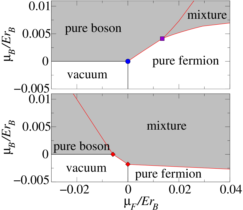
Figure 4: (Color online) Zero temperature phase diagrams for a repulsive ($a_{BF}>0$, top panel) and attractive ($a_{BF}<0$, bottom panel) Bose-Fermi ¹⁷⁴Yb-⁶Li mixture in 1D, i.e., for zero hopping amplitude $t=0$, and for $zeta=0.23$. Differently from the finite $t$ case (cf. Fig. 2), the transition between the pure boson and mixed phase becomes first order (thick red solid line), meeting with the other two first order transition lines (one between the pure fermion and mixed phase and the other between the pure fermion and the pure boson phases) at a triple point (filled violet square), where the three phases coexists. Bottom panel: For an attractive mixture there is neither a triple point nor a tricritical point, rather the first order line crosses the second order line at two critical end-points (filled [red] diamond) delimiting the region of phase separation between the vacuum and a mixed phase.

III.2 Pure 1D limit

Next, we focus on the pure 1D limit, i.e., the limit where the fermions, like the bosons, cannot hop between the tubes (i.e. $t=0$). The phase diagram in chemical potential resulting from minimizing the free energy is shown in Fig. 4, for both repulsive and attractive Bose-Fermi interactions. It can be seen that, in the pure 1D limit, for both repulsive and attractive interspecies interactions, all transitions (except for the trivial ones from the vacuum phase) are discontinuous. In particular, the transition between the pure boson to the mixed phases, which was found to be continuous in the mixed dimensional system, becomes discontinuous as soon as the fermions are confined to 1D. In App. B we carry on an expansion for small fermion density that allows us to establish the nature of the phase transitions where the number of Fermi surfaces changes from zero to one. As shown there, the main difference between the mixed-dimensional case illustrated in the previous section and the pure 1D limit analyzed here can be traced down to the different scaling of the Fermi kinetic energy with the lineal fermion density $\rho^{0}_{F}$ in 1D and 3D. In particular, whereas in 1D the Fermi kinetic energy scales as $(\rho^{0}_{F})^{3}$, in 3D it scales more slowly as $(\rho^{0}_{F})^{5/3}$.

Furthermore, similarly to what was found in the previous section, the fermionization of bosons in 1D also renders the transition between the pure fermion and mixed phases discontinuous. These results are compatible with the previous results obtained by Das in Ref. Das (2003), where was found that the transition between the pure boson and fermion phases is discontinuous thus leading to phase separation.

The main difference between the repulsive and the attractive cases is the way the transitions across which the density of fermions changes connect with the transition between the pure fermion and mixed phase. In particular, in the repulsive case (upper panel of Fig. 4), the three first order transition lines (thick red solid curves) between pure boson-pure fermion, pure fermion-mixed, and pure boson-mixed phases meet at a triple point (filled violet square symbol). At this triple point, the three phases coexist since the free energy exhibits three degenerate local minima (see Fig. 5). On the other hand, for the attractive case (see lower panel of Fig. 4), the triple point is absent. Instead, two critical end points (filled red diamonds) appear. In the density phase diagram, the critical end points delimit a triangularly-shaped region (see bottom panel of Fig. 6), where phase separation occurs between the vacuum and mixed phases. Similarly to conclusion reached in Ref. Marchetti et al. (2009), this region can be regarded as a remnant of the collapse that occurs in the absence of a lattice in 3D Bose-Fermi mixtures with sufficiently large attractive interactions Viverit et al. (2000); Pethick and Smith (2002).

Let us finally remark that 1D Bose-Fermi mixtures in the exactly solvable limit of equal masses (i.e. $m_{B}=m_{F}$) and equal interactions strengths ($g_{BB}^{1D}=g_{BF})$ have been analyzed in Ref. Imambekov and Demler (2006). By relying on a linear stability analysis, which requires that the compressibility matrix must be positively defined for any strength of the interactions, the authors of Ref. Imambekov and Demler (2006) concluded that the system is always stable against demixing. However, in this work, by globally minimizing the system free energy, i.e., by looking for the global energy minima, we find that phase separation occurs in a rather broad region of the density phase diagram and, in particular, it always occurs for small bosons and fermion densities in the pure 1D limit.

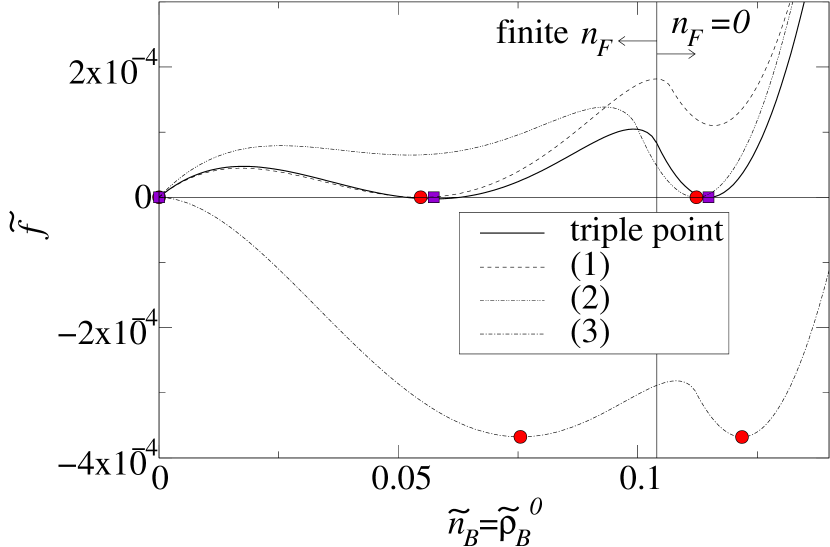
Figure 5: (Color online) Dimensionless free energy density $\tilde{f}$ plotted versus the dimensionless bosonic density $\tilde{n}_{B}=\tilde{\rho}_{B}^{0}$ for fixed dimensionless hopping strength $\tilde{t}=0.023$, fixed interaction parameter $\zeta=0.27$, and a 1D repulsive Bose-Fermi system, corresponding to the density phase diagram shown in the top panel of Fig. 6. The values of the chemical potentials are fixed at the three different first order transition lines near the triple point $(\mu_{B}^{1D}/Er_{B},\mu_{F}/Er_{B})\simeq(35.3,11.2)$, which describes the state where phase separation occurs between the three phases, pure boson, pure fermion and mixed phase: $(1)\simeq(36.3,11.4)$ describe phase separation between pure fermion and mixed phase; $(2)\simeq(33.9,10.8)$ phase separation between pure fermion and pure boson; finally $(3)\simeq(38.1,12.4)$ phase separation between mixed and pure boson.

Figure 6: (Color online) Phase diagrams in the density plane $(\tilde{n}_{B},\tilde{n}_{F})$ for $\zeta=0.27$ and zero hopping strength $t=0$ (same remarks as for Fig. 3 apply). Top panel: for repulsive interactions in the 1D limit, phase separation occurs, not only between a pure fermion and a mixed phase, but also between a pure boson and pure fermion phase, as well as between a pure boson and a mixed phase. Bottom panel: In contrast, for the attractive case, there is no phase separation between pure phases, rather, it exists a region of phase separation between the vacuum and a mixed phase.

IV Conclusions and Outlook

To summarize, we have studied the equilibrium phase diagram of a Bose-Fermi system in a mixed-dimensional geometry of an array of coupled 1D tubes, where bosons are strongly localized along the 1D tubes, while fermions can hop between the tubes. Because we treat the boson interaction term non-perturbatively using the Bethe ansatz, we have found that the transition between the pure Fermi phase and the mixed phase is always first order. This implies that, for this system, phase separation can take place between a pure fermion and a mixed phase. However, the phase transition between pure boson and mixed phases is found to be continuous for finite hoping amplitude of the fermions and phase separation cannot take place between these two phases. This contrasts with the results obtained by assuming that the bosons form a quasi-condensate and thus applying a standard mean-field treatment where the boson density is replaced with its expectation value Marchetti et al. (2009). In that case, the free energy the transition between the pure fermion and a mixed phases can be continuous as well as discontinuous, depending on the system parameters.

In the pure 1D limit, we found that the all transitions are first order, except for the trivial ones between the vacuum state and the pure fermion or boson phases. The main differences introduced by the sign of the interaction are the existence of a triple point for repulsive interactions, and the appearance of two critical end points delimiting a first order line between the mixed and the vacuum phases.

Thus, the main difference between the 1D limit and the mixed dimensional system is the change in the character of the transition between the pure boson and mixed phases. We have argued (see App. B) that this difference is a consequence of the different scaling of the Fermi gas kinetic energy contribution to the free energy function with the fermion density.

Before commenting on the relevance of our findings for the experiments using ¹⁷⁴Yb-⁶Li mixtures, it is interesting to note that, because we have applied the Bethe ansatz to the 1D Bose Hamiltonian $\hat{H}_{B}^{mf}$ (17), we can extend our analysis to to Fermi-Fermi system consisting of a light and a heavy atom. In fact, in the limit $g_{BB}\to+\infty$ where $\gamma\to\infty$, the boson energy, $e(\gamma)$ becomes identical to that of a free Fermi gas Girardeau (1960). By taking this limit of the Bethe-energy in Eq. (26), we found that the phase diagrams for both repulsive and attractive Fermi-Fermi interactions evaluated in the same way as before are qualitatively similar to those displayed in Fig. 2 for the Bose-Fermi mixture and that the differences are small and only quantitative .

The actual experimental systems are rendered inhomogeneous by the existence of harmonic trapping. For mixed dimensionality systems, in general, and the ¹⁷⁴Yb-⁶Li system Hansen et al. (2013); Ivanov et al. (2011); Okano et al. (2010) loaded in an anisotropic optical lattice in particular, we can rely on the local density approximation and deduce the main implications for experiments from the phase diagrams in the chemical potential space shown in Fig. 2 and in Fig. 4. For a given trap frequency and total atom numbers $N_{F}$ and $N_{B}$, it is possible to determine the range of values of the chemical potentials $\mu_{F}$ and $\mu_{B}^{1D}$ of the phase diagrams in Figs. 2 and 4 being sampled by the trapped system. This range determines a region in the chemical phase diagram that contains the possible phases that will coexist in the trap.

Lastly, we comment on the accuracy of the above mean-field approach that we have employed for the Bose-Fermi interaction term. Indeed, as any other mean-field theory, it neglects fluctuations. We expect fluctuations to be especially important close to a phase transition. Nevertheless, as shown later in Sec. III, our calculations indicate that many of the phase transitions in the mixed dimensionality Bose-Fermi system (cf. III.1) and in the pure 1D limit are discontinuous. This means that, even very close to the transition point, fluctuations of the boson and fermion densities are typically suppressed and thus it can be expected that the mean-field theory to give a reliable picture. However, we also numerically observed that some of the transitions are only weakly first order. In other cases, however, the transition was found to be continuous. Therefore a careful assessment of the effect of fluctuations will be required but will not be pursued here.

Furthermore, within the above mean-field approach, we also have neglected the inter-tube couplings as well as the effect of the bosons on the fermion properties, which are as a non-interacting Fermi gas. These are also concerns that deserve to be investigated in the future work. Here, we have assumed that such effects are relatively weak and can only become important only for large values $|a_{BF}|$ and/or very low temperatures that may not be easily achievable under current experimental conditions.

Beyond the assessment the accuracy of the present mean-field approach, another interesting direction is to apply the methods developed here to mixed dimensionality systems where the 1D bosons interact via longer range interactions, such as dipolar gases or are tuned to the so-called the super-Tonks regime Batchelor et al. (2005); Chen et al. (2010); Haller et al. (2009); Qi and Guan (2013); Valiente (2012); Cazalilla et al. (2011).

Appendix A Mean-field approximation

In this appendix, we provide the intermediate steps necessary to obtain the mean-field Hamiltonian, Eq. (16). First of all, let us evaluate the expectation value of the fermion density operator in a tube $\hat{\rho}_{F{\mathbf{R}}}(x)$. By substituting the expression (6) into (11) and using that, for a non-interacting Fermi gas, $\langle\hat{f}^{{\dagger}}_{{\mathbf{k}}}\hat{f}^{\phantom{{\dagger}}}_{{\mathbf{k}}^{\prime}}\rangle=\delta_{{\mathbf{k}},{\mathbf{k}}^{\prime}}n_{{\mathbf{k}}}$, with $n_{{\mathbf{k}}}$ being the Fermi-Dirac distribution function, we obtain:

$$\langle\hat{\rho}_{F{\mathbf{R}}}(x)\rangle=\displaystyle\frac{1}{L}\sum_{{\mathbf{k}}}n_{{\mathbf{k}}}\int d{\mathbf{r}}_{\perp}|\varphi^{\phantom{*}}_{{\mathbf{R}}}({\mathbf{r}}_{\perp})|^{2}|\phi_{{\mathbf{k}}_{\perp}}({\mathbf{r}}_{\perp})|^{2}\;.$$ (30)

Further, we can assume that the fermions occupy only the lowest Bloch band of the square lattice, thus the Bloch wave function $\phi_{{\mathbf{k}}_{\perp}}({\mathbf{r}}_{\perp})$ can be developed in terms of Wannier functions $w^{\phantom{*}}_{{\mathbf{R}}}({\mathbf{r}}_{\perp})$ localized at the ${\mathbf{R}}$-th tube:

$$\phi_{{\mathbf{k}}_{\perp}}({\mathbf{r}}_{\perp})=\displaystyle\frac{1}{\sqrt{N}}\sum_{{\mathbf{R}}}e^{i{\mathbf{k}}_{\perp}\cdot{\mathbf{R}}}w^{\phantom{*}}_{{\mathbf{R}}}({\mathbf{r}}_{\perp})\;,$$ (31)

where $N=N_{y}N_{z}$. Therefore, Eq. (30) reads:

$$\langle\hat{\rho}_{F{\mathbf{R}}}(x)\rangle=\displaystyle\frac{1}{L}\sum_{{\mathbf{k}}}n_{{\mathbf{k}}}\frac{1}{N}\sum_{{\mathbf{R}}^{\prime},{\mathbf{R}}^{\prime\prime}}\int d{\mathbf{r}}_{\perp}e^{i{\mathbf{k}}_{\perp}\cdot({\mathbf{R}}^{\prime}-{\mathbf{R}}^{\prime\prime})}\\ \times w_{{\mathbf{R}}^{\prime}}^{*}({\mathbf{r}}_{\perp})w^{\phantom{*}}_{{\mathbf{R}}^{\prime\prime}}({\mathbf{r}}_{\perp})|\varphi^{\phantom{*}}_{{\mathbf{R}}}({\mathbf{r}}_{\perp})|^{2}\\ \simeq\displaystyle\frac{N_{F}}{L}\frac{1}{N}\int d{\mathbf{r}}_{\perp}|w^{\phantom{*}}_{{\mathbf{R}}}({\mathbf{r}}_{\perp})|^{2}|\varphi^{\phantom{*}}_{{\mathbf{R}}}({\mathbf{r}}_{\perp})|^{2}=\rho^{0}_{F}A\;,$$ (32)

where $N_{F}=\sum_{{\mathbf{k}}}n_{{\mathbf{k}}}$, $\rho^{0}_{F}$ is the 1D density of fermions (15), and

$$A=N\int d{\mathbf{r}}_{\perp}|\varphi^{\phantom{*}}_{{\mathbf{R}}}({\mathbf{r}}_{\perp})|^{2}|\phi_{{\mathbf{k}}_{\perp}}({\mathbf{r}}_{\perp})|^{2}\\ \simeq\displaystyle\frac{1}{N}\int d{\mathbf{r}}_{\perp}|w^{\phantom{*}}_{{\mathbf{R}}}({\mathbf{r}}_{\perp})|^{2}|\varphi^{\phantom{*}}_{{\mathbf{R}}}({\mathbf{r}}_{\perp})|^{2}\;.$$ (33)

In this derivation, we have used the fact that the boson Wannier orbital $\varphi^{\phantom{*}}_{{\mathbf{R}}}({\mathbf{r}}_{\perp})$ is strongly localized around ${\mathbf{r}}_{\perp}={\mathbf{R}}$, thus we have neglected the contributions of the terms ${\mathbf{R}}^{\prime}$ and ${\mathbf{R}}^{\prime\prime}$ different from ${\mathbf{R}}$, because the corresponding wavefunction overlaps are negligible. Note also that the constant $A$ (33) does not depend on the tube index ${\mathbf{R}}$. Further, we can approximate $\varphi^{\phantom{*}}_{{\mathbf{R}}}({\mathbf{r}}_{\perp})\simeq e^{-|{\mathbf{r}}_{\perp}-{\mathbf{R}}|^{2}/2\ell^{2}_{B}}/(\sqrt{\pi}\ell_{B})$ and $w^{\phantom{*}}_{{\mathbf{R}}}({\mathbf{r}}_{\perp})\simeq e^{-|{\mathbf{r}}_{\perp}-{\mathbf{R}}|^{2}/2\ell^{2}_{F}}/(\sqrt{\pi}\ell_{F})$ with $\ell_{B}<\ell_{F}\ll d$, therefore the constant $A$ is given by:

$$A\simeq\frac{1}{\pi(\ell^{2}_{F}+\ell^{2}_{B})}\;.$$ (34)

Taking into account that the mean-field averages of the boson and fermion densities are given by the expressions (13), in order to obtain the final expression of the Hamiltonian, Eq. (16), we need to deal with

$$\sum_{{\mathbf{R}}}\int dx\langle\hat{\rho}_{B{\mathbf{R}}}(x)\rangle\hat{\rho}_{F{\mathbf{R}}}(x)$$ (35)

$$=\rho_{B}^{0}\sum_{{\mathbf{R}}}\sum_{{\mathbf{k}}}\int d{\mathbf{r}}_{\perp}|\varphi^{\phantom{*}}_{{\mathbf{R}}}({\mathbf{r}}_{\perp})|^{2}|\phi_{{\mathbf{k}}_{\perp}}({\mathbf{r}}_{\perp})|^{2}\hat{f}_{{\mathbf{k}}}^{\dagger}\hat{f}^{\phantom{{\dagger}}}_{{\mathbf{k}}}$$ (36)

$$\simeq\rho_{B}^{0}A\sum_{{\mathbf{k}}}\hat{f}_{{\mathbf{k}}}^{\dagger}\hat{f}^{\phantom{{\dagger}}}_{{\mathbf{k}}}\;.$$ (37)

Appendix B Series expansion for small Fermi density

In this appendix we want to carry on an expansion for small fermion density so that to be able to establish the nature of the phase transitions where the number of Fermi surfaces changes from zero to one, such as the phase transition between a pure boson and a mixed phase. This is done in the same spirit to the expansion for small boson density conducted at the end of Sec. III.1 that has allowed us to establish that the transitions between pure fermion and any phase with a finite density of bosons can only be first order.

The starting point is the mean-field Hamiltonian derived in Eq. (16), with the difference that now, to simplify the analysis, we will assume that the fermion dispersion appearing in Eq. (18) is quadratic, $\varepsilon({\mathbf{k}})=k^{2}/2m_{F}$, where ${\mathbf{k}}=k_{x}$ if fermions, like bosons, move strictly in 1D, whereas ${\mathbf{k}}=(k_{x},k_{y},k_{z})$ if we instead consider the mixed-dimensional case where fermions are free to move in all three dimensions, while bosons still move strictly in 1D. Note that assuming a quadratic isotropic dispersion for the fermions is expected to be a good approximation in the small fermion density regime that we are going to consider here, even if the true dispersion in the mixed-dimensional case is anisotropic: In fact, when fermions start to mix with bosons, they must necessarily occupy the lowest band energy levels, for which the dispersion can be approximated as quadratic. The anisotropy can be rescaled out when evaluating the fermion density $\rho^{0}_{F}$ as a function of the Fermi wavevector $k_{F}$, and yields to an overall prefactor relative to the isotropic result.

Considering the mean-field Hamiltonian derived in Eq. (16), the following step is to average over the fermion operator density in the fermion Hamiltonian (18), obtaining the Fermi-Dirac distribution function at zero temperature, $\langle\hat{f}^{{\dagger}}_{{\mathbf{k}}}\hat{f}^{\phantom{{\dagger}}}_{{\mathbf{k}}}\rangle=n_{{\mathbf{k}}}=\theta(k_{F}-k)$. The free energy density we obtain this way will have a different dependence on the Fermi density depending whether fermions move in 1D or 3D.

Let us start considering the case where fermions move in 1D, so that the lineal Fermi density defined in Eq. (15) is $\rho_{F}^{0}=N_{F}/NL=k_{F}/\pi$ and the free energy potential $g=\langle\hat{H}^{mf}\rangle/LN$ reads as:

$$g=\displaystyle\frac{\pi^{2}}{6m_{F}}(\rho^{0}_{F})^{3}-\left(\mu_{F}-g_{BF}A\rho^{0}_{B}\right)\rho^{0}_{F}+\\ \frac{(\rho_{B}^{0})^{3}}{2m_{B}}e(\gamma)-\mu_{B}^{1D}\rho_{B}^{0}\;.$$ (38)

Note that now the free energy potential $g=g(\mu_{B}^{1D},\mu_{F},\rho_{B}^{0},\rho_{F}^{0})$ depends on both the boson and fermion densities as well as on the chemical potentials. This means that minimizing $g$ with respect to the fermion density,

$$f(\mu_{B}^{1D},\mu_{F},\rho_{B}^{0})=\min_{\rho^{0}_{F}}g(\mu_{B}^{1D},\mu_{F},\rho_{B}^{0},\rho_{F}^{0})\;,$$ (39)

we retrieve the free energy potential $f(\mu_{B}^{1D},\mu_{F},\rho_{B}^{0})$ considered in Eq. (19), which global minimum with respect to the boson density gives the true thermodynamic grand-canonical free energy density (22).

However, if we instead minimize $g(\mu_{B}^{1D},\mu_{F},\rho_{B}^{0},\rho_{F}^{0})$ with respect to the boson density,

$$h(\mu_{B}^{1D},\mu_{F},\rho_{F}^{0})=\min_{\rho^{0}_{B}}g(\mu_{B}^{1D},\mu_{F},\rho_{B}^{0},\rho_{F}^{0})\;,$$ (40)

so that to eliminate $\rho^{0}_{B}$ in favor of $\rho^{0}_{F}$, $\mu_{F}$ and $\mu_{B}^{1D}$, then the free energy potential $h(\mu_{B}^{1D},\mu_{F},\rho_{F}^{0})$ thus obtained can be used to study the phase transitions where the number of Fermi surfaces changes from zero to one, by expanding for small values of $\rho^{0}_{F}$. Because the dimensionless function $e(\gamma)$ coming from the Bethe ansatz is determined numerically, this plan of deriving the free energy potential $h(\mu_{B}^{1D},\mu_{F},\rho_{F}^{0})$ is not a trivial one. However, we can carry on this procedure in two opposite limits, corresponding to high ($\gamma=m_{B}g_{BB}^{1D}/\rho_{B}^{0}\ll 1$) and low ($\gamma\gg 1$) density, respectively:

$$e(\gamma)\simeq\begin{cases}\gamma&\gamma\ll 1\\ e_{TG}=\frac{\pi^{2}}{3}&\gamma\gg 1\;.\end{cases}$$ (41)

Note that the last limit results in a contribution to the free energy potential $h$ of $\pi^{2}(\rho^{0}_{B})^{3}/6m_{B}$, which is identical to the kinetic energy of a free 1D Fermi gas. This is the result of fermionization in the Tonks-Girardeau limit Cazalilla et al. (2011).

Evaluating (40) by solving $\partial g/\partial\rho^{0}_{B}=0$ for $\rho^{0}_{B}$, in both cases of high and low boson density, we obtain a series in terms of the Fermi density of cubic form:

$$h=h_{0}+h_{2}\rho^{0}_{F}+h_{4}(\rho^{0}_{F})^{2}+h_{6}(\rho^{0}_{F})^{3}+\cdots\;.$$ (42)

For high boson density the coefficients, for $\mu_{B}^{1D}>Ag_{BF}\rho^{0}_{F}$, which requires $\mu_{B}^{1D}$ and $g_{BF}$ to have the same sign, are given by

$$h_{2} =\frac{Ag_{BF}}{g^{1D}_{BB}}\mu_{B}^{1D}-\mu_{F}$$ (43)

$$h_{4} =-\frac{A^{2}g^{2}_{BF}}{2g^{1D}_{BB}}$$ (44)

$$h_{6} =\frac{\pi^{2}}{6m_{F}}\;.$$ (45)

In the low boson density limit, instead, we obtain (also for $\mu_{B}^{1D}>Ag_{BF}\rho^{0}_{F}$) that the coefficients of the expansion (42) are now given by

$$h_{2} =\frac{Ag_{BF}}{\pi}\sqrt{2m_{B}\mu_{B}^{1D}}-\mu_{F}$$ (46)

$$h_{4} =-\frac{A^{2}g^{2}_{BF}\sqrt{m_{B}}}{2\pi\sqrt{2\mu_{B}^{1D}}}$$ (47)

$$h_{6} =\frac{\pi^{2}}{6m_{F}}-\frac{A^{3}g_{BF}^{3}\sqrt{m_{B}}}{12\sqrt{2}\pi{\mu_{B}^{1D}}^{3/2}}\;.$$ (48)

In this last case, note that, for $m_{F}\ll m_{B}$, as we have assumed in the main text, the coefficient of the cubic term is expected to be positive and large. In both cases, while $h_{6}>0$, the coefficient of the square term is always negative, $h_{4}<0$, implying that the transition cannot be continuous, rather it is first order. For small fermion density, the transition has place for $h_{2}>0$ and $h_{4}=-2\sqrt{h_{2}h_{6}}$, implying that, for large values of the coefficient $h_{6}$, $h_{2}\to 0$ and the transition is weakly first order, as we have indeed observed numerically in many cases.

The $\rho^{0}_{F}$ expansion just carried on thus allows us to understand the nature of the transition between the pure Bose gas and mixed phases and deduce that it has to be first order in the strictly 1D limit. We can merge this result with the one obtained in Sec. III.1, where we were expanding for small boson density (Tonks-Girardeau limit), and found that the transition between the pure Fermi gas and the mixed phases is also first order. We can thus conclude that in the 1D limit the transitions between the pure boson/fermion phases and the mixed phase, must be all first order.

For comparison purposes, we can now consider the case of mixed dimensionality, i.e., where fermions move in 3D. Now, the 3D Fermi density is given by $N_{F}/\Omega=\rho^{0}_{F}d^{-2}=k_{F}^{3}/6\pi^{2}$, where the volume is $\Omega=Nd^{2}L$, $d$ is the spacing between the tubes (cf. Fig 1), and $\rho^{0}_{F}$ the lineal fermion density. Thus the kinetic energy contribution to the free energy potential $g=\langle\hat{H}^{mf}\rangle/LN$ now scales differently than in the 1D limit:

$$g=\displaystyle\frac{d^{2}(6\pi^{2}d^{-2}\rho^{0}_{F})^{5/3}}{20\pi^{2}m_{F}}-\left(\mu_{F}-g_{BF}A\rho^{0}_{B}\right)\rho^{0}_{F}+\\ \frac{(\rho_{B}^{0})^{3}}{2m_{B}}e(\gamma)-\mu_{B}^{1D}\rho_{B}^{0}\;.$$ (49)

As before, we eliminate the boson density $\rho^{0}_{B}$ from the potential $g$ by making use of (40) and then we expand for small values of the Fermi density $\rho^{0}_{F}$. In this case we obtain:

$$h=h_{0}+h_{2}\rho^{0}_{F}+h_{10/3}(\rho^{0}_{F})^{5/3}+\cdots\;,$$ (50)

where the coefficient $h_{2}$ is given by the expressions (43) for the high boson density, while by (46) for the low boson density limit. The coefficient $h_{10/3}$ is in both cases instead given by:

$$h_{10/3}=\displaystyle\frac{d^{-4/3}(6\pi^{2})^{5/3}}{20\pi^{2}m_{F}}\;.$$ (51)

We can thus see that, while the coefficient $h_{2}$ can change sign depending on the values of the system parameters, the coefficient of the next order term, which scales like $(\rho^{0}_{F})^{5/3}$ rather than quadratically, is always positive $h_{10/3}>0$. This means that the position of the closest minimum to $\rho^{0}_{F}=0$ is entirely controlled by the sign of $h_{2}$, that is, the transition between the pure boson and mixed phases must be continuous. By contrast, as we have argued in Sec. III.1, the transition between the pure fermion and the mixed phase is independent on the dimensionality where fermions live and is always first order.

The main conclusion of the simple exercise carried on in this appendix is that the different nature of the phase transitions where the number of Fermi surfaces changes from zero to one between the strictly 1D case and the mixed-dimensional case is a consequence of the different scaling of the fermion kinetic energy in 1D and in 3D. Note that this result is also applicable to the transitions between the pure fermion and mixed phases, as bosons in 1D at low density behave as a free Fermi gas by virtue of fermionization.

References

- Pethick and Smith (2002) C. J. Pethick and H. Smith, Bose-Einstein condensation in dilute gases (Cambridge University Press, 2002).
- Courteille et al. (1998) P. Courteille, R. S. Freeland, D. J. Heinzen, F. A. van Abeelen, and B. J. Verhaar, Phys. Rev. Lett. 81, 69 (1998).
- Inouye et al. (1998) S. Inouye, M. R. Andrews, J. Stenger, H. J. Miesner, D. M. Stamper-Kurn, and W. Ketterle, Nature 392, 151 (1998).
- Bloch et al. (2008) I. Bloch, J. Dalibard, and W. Zwerger, Rev. Mod. Phys. 80, 885 (2008).
- Mølmer (1998) K. Mølmer, Phys. Rev. Lett. 80, 1804 (1998).
- Viverit et al. (2000) L. Viverit, C. J. Pethick, and H. Smith, Phys. Rev. A 61, 053605 (2000).
- Wang et al. (2006) D.-W. Wang, M. D. Lukin, and E. Demler, Phys. Rev. Lett. 97, 180413 (2006).
- Wang (2007) D.-W. Wang, Phys. Rev. Lett. 98, 060403 (2007).
- Huang and Wang (2009) Y.-P. Huang and D.-W. Wang, Phys. Rev. A 80, 053610 (2009).
- Santos et al. (2000) L. Santos, G. V. Shlyapnikov, P. Zoller, and M. Lewenstein, Phys. Rev. Lett. 85, 1791 (2000).
- Micheli et al. (2006) A. Micheli, G. K. Brennen, and P. Zoller, Nature Physics 2, 341 (2006).
- Büchler et al. (2007) H. P. Büchler, E. Demler, M. Lukin, A. Micheli, N. Prokof’ev, G. Pupillo, and P. Zoller, Phys. Rev. Lett. 98, 060404 (2007).
- DeMille (2002) D. DeMille, Phys. Rev. Lett. 88, 067901 (2002).
- Greiner et al. (2002) M. Greiner, O. Mandel, T. Esslinger, T. W. H. Hänsch, and I. Bloch, Nature 415, 39 (2002).
- Posazhennikova (2006) A. Posazhennikova, Rev. Mod. Phys. 78, 1111 (2006).
- Martiyanov et al. (2010) K. Martiyanov, V. Makhalov, and A. Turlapov, Phys. Rev. Lett. 105, 030404 (2010).
- Moritz et al. (2005) H. Moritz, T. Stöferle, K. Günter, M. Köhl, and T. Esslinger, Phys. Rev. Lett. 94, 210401 (2005).
- Kinoshita (2004) T. Kinoshita, Science 305, 1125 (2004).
- Paredes et al. (2004) B. Paredes, A. Widera, V. Murg, O. Mandel, S. Fölling, I. Cirac, G. V. Shlyapnikov, T. W. H. Hänsch, and I. Bloch, Nature 429, 275 (2004).
- Cazalilla et al. (2011) M. A. Cazalilla, R. Citro, T. Giamarchi, E. Orignac, and M. Rigol, Rev. of Mod. Phys. 83, 1405 (2011).
- Nishida and Tan (2008) Y. Nishida and S. Tan, Phys. Rev. Lett. 101, 170401 (2008).
- Yang et al. (2011) X. S. Yang, B. B. Huang, and S. L. Wan, Eur. Phys. J. B 83, 445 (2011).
- Lamporesi et al. (2010) G. Lamporesi, J. Catani, G. Barontini, Y. Nishida, M. Inguscio, and F. Minardi, Phys. Rev. Lett. 104, 153202 (2010).
- Minardi et al. (2011) F. Minardi, G. Barontini, J. Catani, G. Lamporesi, Y. Nishida, and M. Inguscio, Journal of Physics: Conference Series 264, 012016 (2011).
- Marchetti et al. (2009) F. Marchetti, T. Jolicoeur, and M. Parish, Phys. Rev. Lett. 103, 105304 (2009).
- Albus et al. (2003) A. Albus, F. Illuminati, and J. Eisert, Phys. Rev. A 68, 023606 (2003).
- Viverit and Giorgini (2002) L. Viverit and S. Giorgini, Phys. Rev. A 66, 063604 (2002).
- Modugno et al. (2003) M. Modugno, F. Ferlaino, F. Riboli, G. Roati, G. Modugno, and M. Inguscio, Phys. Rev. A 68, 043626 (2003).
- Günter et al. (2006) K. Günter, T. Stöferle, H. Moritz, M. Köhl, and T. Esslinger, Phys. Rev. Lett. 96, 180402 (2006).
- Büchler and Blatter (2004) H. Büchler and G. Blatter, Phys. Rev. A 69, 063603 (2004).
- Das (2003) K. Das, Phys. Rev. Lett. 90, 170403 (2003).
- Lai and Yang (2011) C. K. Lai and C. N. Yang, Phys. Rev. A 3, 393 (2011).
- Cazalilla and Ho (2003) M. Cazalilla and A. Ho, Phys. Rev. Lett. 91, 150403 (2003).
- Mathey et al. (2004) L. Mathey, D. W. Wang, W. Hofstetter, M. Lukin, and E. Demler, Phys. Rev. Lett. 93, 120404 (2004).
- Imambekov and Demler (2006) A. Imambekov and E. Demler, Phys. Rev. A 73, 021602(R) (2006).
- Zaccanti et al. (2006) M. Zaccanti, C. D’Errico, F. Ferlaino, G. Roati, M. Inguscio, and G. Modugno, Phys. Rev. A 74, 041605(R) (2006).
- Modugno (2007) G. Modugno, arXiv:cond-mat/0702277 (2007).
- Zirbel et al. (2008) J. J. Zirbel, K. K. Ni, S. Ospelkaus, J. P. D’Incao, C. E. Wieman, J. Ye, and D. S. Jin, Phys. Rev. Lett. 100, 143201 (2008).
- Jaksch et al. (1998) D. Jaksch, C. Bruder, J. I. Cirac, C. W. Gardiner, and P. Zoller, Phys. Rev. Lett. 81, 3108 (1998).
- Stöferle et al. (2004) T. Stöferle, H. Moritz, C. Schori, M. Köhl, and T. Esslinger, Phys. Rev. Lett. 92, 130403 (2004).
- Kinoshita et al. (2005) T. Kinoshita, T. Wenger, and D. S. Weiss, Phys. Rev. Lett. 95, 190406 (2005).
- Tan (2012) S. Tan, Phys. Rev. Lett. 109, 020401 (2012).
- Malatsetxebarria et al. (2013) E. Malatsetxebarria, Z. Cai, U. Schöllwock, and M. A. Cazalilla, In preparation (2013).
- Hansen et al. (2013) A. H. Hansen, A. Y. Khramov, W. H. Dowd, A. O. Jamison, B. Plotkin-Swing, R. J. Roy, and S. Gupta, Phys. Rev. A 87, 013615 (2013).
- Ivanov et al. (2011) V. V. Ivanov, A. Khramov, A. H. Hansen, W. H. Dowd, F. Münchow, A. O. Jamison, and S. Gupta, Phys. Rev. Lett. 106, 153201 (2011).
- Okano et al. (2010) M. Okano, H. Hara, M. Muramatsu, K. Doi, S. Uetake, Y. Takasu, and Y. Takahashi, Applied Physics B: Lasers and Optics 98, 691 (2010).
- Chin et al. (2006) J. K. Chin, D. E. Miller, Y. Liu, C. Stan, W. Setiawan, C. Sanner, K. Xu, and W. Ketterle, Nature 443, 961 (2006).
- Olshanii (1998) M. Olshanii, Phys. Rev. Lett. 81, 938 (1998).
- Moritz et al. (2003) H. Moritz, T. Stöferle, M. Köhl, and T. Esslinger, Phys. Rev. Lett. 91, 250402 (2003).
- Cazalilla et al. (2006) M. A. Cazalilla, A. F. Ho, and T. Giamarchi, New Journal of Physics 8, 158 (2006).
- Lieb and Liniger (1963) E. H. Lieb and W. Liniger, Physical Review 130, 1605 (1963).
- Takahashi (2013) Y. Takahashi, Private Communication (2013).
- Kitagawa et al. (2008) M. Kitagawa, K. Enomoto, K. Kasa, Y. Takahashi, R. Ciuryło, P. Naidon, and P. Julienne, Phys. Rev. A 77, 012719 (2008).
- Sachdev (2010) S. Sachdev, Quantum Phase Transitions (Cambridge University Press, 2010), 2nd ed.
- Cazalilla (2003) M. Cazalilla, Phys. Rev. A 67, 053606 (2003).
- Girardeau (1960) M. Girardeau, J. Math. Phys. 1, 516 (1960).
- Batchelor et al. (2005) M. T. Batchelor, M. Bortz, X. W. Guan, and N. Oelkers, Journal of Statistical Mechanics: Theory and Experiment 2005, L10001 (2005).
- Chen et al. (2010) S. Chen, X.-W. Guan, X. Yin, L. Guan, and M. T. Batchelor, Phys. Rev. A 81, 031608 (2010).
- Haller et al. (2009) E. Haller, M. Gustavsson, M. J. Mark, J. G. Danzl, R. Hart, G. Pupillo, and H. C. Nägerl, Science 325, 1224 (2009).
- Qi and Guan (2013) R. Qi and X. Guan, Europhys. Lett. 101, 40002 (2013).
- Valiente (2012) M. Valiente, Europhys. Lett. 98, 10010 (2012).