Time dependent black holes and scalar hair

Abstract:

We show how to correctly account for scalar accretion onto black holes in scalar field models of dark energy by a consistent expansion in terms of a slow roll parameter. At leading order, we find an analytic solution for the scalar field within our Hubble volume which is regular on both black hole and cosmological event horizons, and compute the back reaction of the scalar on the black hole, calculating the resulting expansion of the black hole. Our results are independent of the relative size of black hole and cosmological event horizons. We comment on the implications for more general black hole accretion, and the no hair theorems.

1 Introduction

Black holes are one of the most fascinating objects in classical general relativity. They represent the endpoint of gravitational collapse of a large mass object, independent of initial conditions. The prototypical black hole, the Schwarzschild solution, was first presented barely a year after Einstein put forward his new theory of gravity, yet it took half a century before relativists were confident of the interpretation of this solution, and began to construct a rigorous set of theorems describing the properties of black holes. One of the more poetically labelled set – the “no hair” theorems [1] – has been perhaps the most contentious. Originally demonstrated for static vacuum black holes, [2, 3], the no hair theorems have been refined and extended to a wide range of interacting particle and gravitational theories, [4, 5, 6]. Nonetheless, there are many known “violations” of the no hair theorems, from the dressing of black holes by scalar or gauge condensates [7], to literal hair, in the form of topological defects which extend out from the black hole to infinity, [8].

The issue of the most basic hair however, scalar hair, is thought to be understood, yet is perhaps the most perplexing. For a wide range of potentials, it is easy to show that a static black hole cannot have a nontrivial scalar field on its event horizon (unless the space-time is asymptotically anti-de Sitter, [9], or the scalar potential has been specifically tailored, [10]). However, within cosmology, scalar fields are widely used, not only for inflation, but as an expedient model of quintessence, [11], or late time acceleration (see [12] for a review of dark energy models). Indeed, the standard exponential scalar potential - widely used to give power law acceleration, was shown to be in conflict with spherically symmetric asymptotically flat or de Sitter static black hole space-times, [13]. How then can these cosmological scalars interact with a black hole event horizon? Generally, the scalar field is varying on a very slow time scale relative to the light crossing time of the black hole, thus we might expect that it has little effect on the event horizon itself, yet, like the inexorable flow of time, the scalar must evolve cosmologically, and it seems contradictory that it is pinned to a single value for all time at the black hole – an issue explored by Barrow, [14], in the context of primordial black holes.

In fact, the resolution of the conflict is quite straightforward: The no hair theorems were explored in the context of static black holes, and quite clearly a rolling cosmological scalar can never be static. Correspondingly, the presence of a black hole in a cosmology implies that the cosmology cannot be spatially homogeneous, and therefore does not have the canonical FRW form. While we can use cosmological perturbation theory to describe the far field effect of the black hole, we cannot describe the full spatial geometry including the event horizon within the context of perturbation theory – and it is the effect of the event horizon which is critical in determining the behaviour of the scalar. We therefore need a time-dependent black hole solution.

Exact black hole solutions are surprisingly thin on the ground, given how ubiquitous black hole are in nature, and time dependent ones even more so. The first dynamical black hole ‘solution’ was postulated by McVittie, [15], who modified the Schwarzschild solution to include an FRW-like cosmology, with the black hole event horizon at fixed comoving radius and a fluid energy density dependent only on time. However, as pointed out in [16], one expects the black hole to break the spatial homogeneity of the cosmology, and thus (except in the special case of a de Sitter universe) this unrealistic set-up leads to a singularity on the would be event horizon. The McVittie solution has been generalised, [17, 18], to allow for radial accretion, although the generalisations follow the method of ‘metric engineering’, in that a specific ansatz is proposed, then the matter stress energy inferred (see also [19] for a discussion of some possible issues with these approaches).

Instead of imposing a particular metric ansatz, a successful approach has been instead to postulate a particular format for the behaviour of the solution, notably self-similarity, first used to estimate primordial black hole accretion in [20], but also extended to allow more general perfect fluid equations of state, [21, 22, 23], and scalar tensor gravity, [24]. Although these solutions do make an assumption about the behaviour of the metric, and are restricted to a perfect fluid, they have the advantage that they are exact, allow for time-dependence of the black hole, to be explored without resorting to complex numerical methods. (See [25] for a brief review.)

There is also the time dependent Vaidya solution, [26], which is somewhat special, as the mass of the black hole now becomes dependent on a null coordinate, requiring a null matter source. There are also exact solutions for Einstein plus scalar field which either represent a collapsing scalar field, [27], or use solution generating techniques to add scalar profiles to a black hole, [28]. In both cases however, the would be event horizon is singular, and indeed in [27], identifying event horizons becomes an issue. Thus a direct approach to finding an exact solution seems to have been unsuccessful in the sense that in cosmology, we expect a solution which will be locally interpretable as a “black hole” (Schwarzschild solution) but that nonetheless will also have large scale cosmological evolution, which on long time scales will give a natural evolution of the black hole event horizon area due to scalar accretion. (See [29] for a review and discussion of the interplay between cosmological expansion and local systems).

Another approach in the literature is to find a probe solution for the scalar field, i.e. one in which the scalar field evolves on a Schwarzschild background, [30, 31]. Here, near the event horizon, the scalar field must be a function of the advanced null coordinate, $v\sim e^{t+r^{*}}$, which parametrises the black hole future event horizon. One can then estimate the back-reaction on the event horizon using the energy momentum of this approximate solution. A problem with this approach however, is that the coordinates being used are local static Schwarzschild coordinates, which do not correspond to the cosmological flow of time at large distances and therefore give no guarantee that any ‘solution’ will be well behaved at cosmological event horizons. One can also worry that estimates using local intuitive notions of energy, rather than an analysis of the Einstein equations with a scalar source, might be misleading.

In order to be confident that probe calculations give a good estimate of scalar accretion onto black holes, we require a time-dependent scalar field with a time dependent black hole. Here, we present a resolution of this problem, by expanding the equations of motion for the geometry and the scalar field order by order in a “slow roll” parameter. We present a procedure for solving for the time dependent scalar on the black hole, finding the leading order solution which extends from the near black hole expectation of [30, 31] to the cosmological solution at large distances. Our solution is valid independent of the relative sizes of the black hole and cosmological event horizons. We also present the back reaction of the scalar field on the black hole, and calculate the expansion rate of the black hole due to scalar accretion. An advantage of our method is that we can identify the event horizons accurately as null surfaces, therefore the usual ambiguity of apparent vs. event horizons does not occur.

It is perhaps worth emphasising that our approach is explicitly to construct a natural extension of the Schwarzschild ‘vacuum’ solution, and not some engineered exact solution of Einstein’s equations, either by making a metric ansatz, or by taking an ansatz for the behaviour of the solution. Our only input will be the symmetries of the physical set-up, and the output a nonsingular solution corresponding to the physical set-up of an FRW expanding universe at large scales, and a (Schwarzschild) black hole with some local scalar field on small scales.

2 Scalar fields and black holes: set-up

In this section, we set up the equations of motion for the scalar field with the black hole. The idea is to write down the general equations of motion compatible with the symmetries, then to expand them order by order in the kinetic energy of the scalar field.

To motivate our approach, consider a universe in which the acceleration of the universe is driven by a slowly rolling scalar field, somewhat analogous to inflation though clearly at a much lower scale. A simple toy model consists of an FRW universe,

$$ds^{2}=dt^{2}-a^{2}(t)d{\bf x}^{2}$$ (1)

and a scalar field with an exponential potential $W=M^{4}e^{-\beta\phi}$, which leads to a power law acceleration

$$a(t)=\left(\frac{t}{t_{0}}\right)^{k}\;\;,\;\;\;\;\;\phi=\phi_{0}+\frac{2}{\beta}\ln\frac{t}{t_{0}}\;\;,\;\;\;\;\;k=\frac{2\kappa}{\beta^{2}}=\frac{2W(\phi)^{2}}{M_{p}^{2}W^{\prime}(\phi)^{2}}=\varepsilon^{-1}$$ (2)

where $\kappa=8\pi G=M_{p}^{-2}$, and $\varepsilon$ is the conventional slow roll parameter introduced here to emphasise that $k\gg 1$.

Now consider the solution in conformal time $\eta=\eta_{0}(t/t_{0})^{(\varepsilon-1)/\varepsilon}$:

$$ds^{2}=\left[\frac{\eta_{0}}{\eta}\right]^{2+\frac{2\varepsilon}{1-\varepsilon}}\left[(d\eta-d\rho)(d\eta+d\rho)-\rho^{2}d\Omega_{{\rm II}}^{2}\right]$$ (3)

where $d\Omega_{{\rm II}}^{2}$ is the standard line element on the unit sphere, and

$$\phi=\phi_{0}-\frac{2\varepsilon}{\beta(1-\varepsilon)}\ln\frac{\eta}{\eta_{0}}\;.$$ (4)

Then, if we assume that $\varepsilon\ll 1$, and expand $[\eta_{0}/\eta]^{\frac{2\varepsilon}{1-\varepsilon}}\sim 1-2\varepsilon\ln|\eta/\eta_{0}|$, this metric is perturbatively close to the de Sitter (dS) metric:

$$g_{ab}=g^{(DS)}_{ab}\left(1-2\varepsilon\ln\left|\frac{\eta}{\eta_{0}}\right|+{\cal O}(\varepsilon^{2})\right)$$ (5)

over a Hubble time interval. The dark energy universe can therefore be expressed as a linear perturbation of a known exact solution to Einstein’s equations – the de Sitter universe. Looking at (4), we see that $\phi=\phi_{0}$, plus a correction of order ${\cal O}\left(\varepsilon^{1/2}M_{p}\right)$, and thus for small $\varepsilon$, we can express the cosmology as a de Sitter universe with a small correction of order ${\cal O}(\varepsilon^{1/2})$ for the scalar, and ${\cal O}(\varepsilon)$ for the geometry.

Now consider adding a black hole to this cosmological rolling scalar solution. Given that the background solution is a perturbation of a de Sitter universe, it is reasonable to suppose that the black hole plus scalar might be expressible as a perturbation of a Schwarzschild de Sitter space-time. Note however, that this is distinct from conventional cosmological perturbation theory, where one perturbs a given spatial section and evolves forward in time. Rather, here we seek to write the fully interacting black hole-plus-scalar system as a perturbation expansion around the static solution in the kinetic motion of the scalar. Just as the rolling scalar cosmology is perturbatively close to the de Sitter manifold, we expect that the rolling scalar plus black hole manifold should be close to the Schwarzschild de Sitter manifold, and just as the linear expansion above has a range of validity, we expect that our expansion will also be valid only over Hubble time-scales.

The geometry of the time-dependent black hole will not now have constant curvature spatial slices, but we do expect an SO$(3)$ symmetry, corresponding to the spherical symmetry of the black hole. We also expect both time and radial dependence in the metric. The general metric may therefore be written in the form [32, 33]

$$ds^{2}=4e^{2\nu}B^{-1/2}dUdV-Bd\Omega_{{\rm II}}^{2}.$$ (6)

This form of the metric elucidates both the symmetry of the space-time (SO(3)), as well as the remaining gauge freedom (the conformal group in the $U,V$ directions). By rewriting the coordinates in light-cone form, it will be clear how to deal with the event horizons present in the anticipated solution (the cosmological and black hole event horizons), as well as how to change gauge to analytically extend across these horizons. In particular, the null coordinates allow us to identify the actual event horizons of the solution, as opposed to apparent horizons, as an horizon is of course always a null surface, defined by $U$ or $V=$ constant.

Using (6), the coupled Einstein-scalar equations for the variables $B,\nu,\phi$ are

$$\phi_{,UV} = -W_{,\phi}(\phi)B^{-1/2}e^{2\nu}-\frac{1}{2B}\left(B_{,U}\phi_{,V}+B_{,V}\phi_{,U}\right)$$ (7)

$$B_{,UV} = 2\left(\kappa W(\phi)B^{1/2}-B^{-1/2}\right)e^{2\nu}$$ (8)

$$\nu_{,UV} = \frac{1}{2}\left(\kappa W(\phi)B^{-1/2}+B^{-3/2}\right)e^{2\nu}-\frac{\kappa}{2}\phi_{,U}\phi_{,V}$$ (9)

$$B_{,VV} = 2\nu_{,V}B_{,V}-\kappa B\phi_{,V}^{2}$$ (10)

$$B_{,UU} = 2\nu_{,U}B_{,U}-\kappa B\phi_{,U}^{2}$$ (11)

where $W(\phi)$ is a general potential, the only stipulation being that it satisfies the slow roll condition $\varepsilon\ll 1$.

For a constant scalar field (i.e. briefly ignoring (7)) a generalisation of the Birkhoff theorem shows that the Einstein equations have Schwarzschild de Sitter (SdS) as a general solution, [32]. Given that we follow a similar procedure in analysing the rolling scalar, it is worth briefly reviewing the steps of this argument.

If $\phi$ is constant, (10) and (11) can be integrated directly to give

$$2\nu=\ln B_{,V}+\ln G^{\prime}(U)=\ln B_{,U}+\ln F^{\prime}(V)$$ (12)

where $F^{\prime}$ and $G^{\prime}$ represent arbitrary integration functions. Consistency of these expressions leads us to deduce that $B$ must be a function of $\left[F(V)+G(U)\right]$, and hence

$$e^{2\nu}=F^{\prime}(V)G^{\prime}(U)B^{\prime}(F+G)\,.$$ (13)

Inserting into (8) then gives

$$F^{\prime}G^{\prime}B^{\prime\prime} =2F^{\prime}G^{\prime}B^{\prime}\left(\kappa W_{0}B^{1/2}-B^{-1/2}\right)$$ (14)

$$\Rightarrow\quad B^{\prime} =\frac{4}{3}\kappa W_{0}B^{3/2}-4B^{1/2}+8GM$$

where $8GM$ is an integration constant (suggestively labeled!), $W_{0}=W(\phi_{0})$, and primes denote differentiation with respect to the argument of the function. However, writing $N(r)$ as the SdS potential

$$N(r)=1-\frac{2GM}{r}-H^{2}r^{2}$$ (15)

shows that in fact

$$B^{\prime}=-4\sqrt{B}N(\sqrt{B})$$ (16)

with $H^{2}=\kappa W_{0}/3$, the vacuum density of the constant scalar field. Changing coordinates to $r=B^{1/2}$, $t=2(G(U)-F(V))$, then gives

$$ds^{2}=\frac{F^{\prime}G^{\prime}B^{\prime}}{B^{1/2}}4dUdV-Bd\Omega_{{\rm II}}^{2}\to N(r)dt^{2}-\frac{dr^{2}}{N(r)}-r^{2}d\Omega_{{\rm II}}^{2}$$ (17)

i.e. the Schwarzschild de Sitter metric in static coordinates. In this form, we can see explicitly that the arbitrary integration functions $F$ and $G$ are simply gauge degrees of freedom of the metric (17), and in fact represent the conformal transformations on the $(U,V)-$plane. Since $B^{\prime}$ can vanish, this metric will in general have singularities at certain values of $B$. These are none other than the black hole and cosmological event horizons of the static co-ordinates. However, “cosmological” coordinates at large ‘$r$’ would not have an horizon, and would asymptote a standard cosmological de Sitter space-time; we therefore need to identify the (Kruskal) transformations which provide extensions across each horizon.

Writing $r^{*}$ as the usual tortoise co-ordinate, note that

$$r^{*}=\int\frac{dr}{N(r)}=-2\int\frac{dB}{B^{\prime}}=-2(F+G)$$ (18)

thus $t-r^{*}=4G$, $t+r^{*}=-4F$. Following the usual Kruskal method, we now choose the functions $F(V)$ and $G(U)$ to make the metric regular at the cosmological event horizon $r_{c}$:

$$F(V) =-\frac{1}{2N^{\prime}(r_{c})}\ln\left[N^{\prime}(r_{c})V\right]\;,\;\; {\rm or}\;\;V =R_{c}\exp\left[\frac{(t+r^{*})}{2R_{c}}\right]$$ (19)

$$G(U) =\frac{1}{2N^{\prime}(r_{c})}\ln\left[N^{\prime}(r_{c})U\right]\;,\;\; {\rm or}\;\;U =R_{c}\exp\left[\frac{(t-r^{*})}{2R_{c}}\right]$$

where we have written $R_{c}=1/N^{\prime}(r_{c})$ as shorthand (see appendix).

Thus, the original functions of the metric (6) are

$$B(U,V) =r^{2}=\left({r^{*}}^{-1}\left[R_{c}\ln\frac{V}{U}\right]\right)^{2}$$ (20)

$$e^{2\nu} =F^{\prime}G^{\prime}B^{\prime}=\frac{R_{c}^{2}\sqrt{B}N(\sqrt{B})}{UV}=\frac{R_{c}^{2}}{UV}rN(r)$$

where ${r^{*}}^{-1}$ is the inverse tortoise function, which does not in general have a closed analytic form, and $r$ is understood to be a function of $U$ and $V$. In these co-ordinates, as $r\to r_{c}$,

$$V=U\exp\left[\frac{r^{*}}{R_{c}}\right]\approx U(r-r_{c})$$ (21)

thus the cosmological event horizon is at $V=0$ and is parametrized by $U$. Moreover

$$e^{2\nu}=-\frac{R_{c}^{2}}{U^{2}}\frac{r_{c}N}{(r-r_{c})}$$ (22)

is explicitly regular as expected.

For future reference, the Kruskal extension at the black hole event horizon $r_{h}$ would be given by the null co-ordinate choice

$$F(v) =-\frac{1}{2N^{\prime}(r_{h})}\ln\left[N^{\prime}(r_{h})v\right]\;,\;\; {\rm or}\;\;v =R_{h}\exp\left[\frac{(t+r^{*})}{2R_{h}}\right]$$ (23)

$$G(u) =-\frac{1}{2N^{\prime}(r_{h})}\ln\left[-N^{\prime}(r_{h})u\right]\;,\;\; {\rm or}\;\;u =R_{h}\exp\left[-\frac{(t-r^{*})}{2R_{h}}\right]$$

writing $R_{h}=1/N^{\prime}(r_{h})$ as before. The black hole event horizon is at $u=0$, and parametrized by $v$. We will mostly work with the ‘cosmological’ co-ordinates $U$ and $V$, however, we will refer to the black hole Kruskals $(u,v)$ when checking regularity at the event horizon.

Now suppose that we take into account that $\phi$ is not constant, and write

$$\phi =\phi_{0}+\sqrt{2\varepsilon}M_{p}\phi_{1}(U,V)$$ (24)

$$B =r^{2}\left(1+\varepsilon\delta_{1}(U,V)\right)$$

$$\nu =\nu_{0}+\varepsilon\delta_{2}(U,V)$$

then, recalling the expressions for $B_{0}=r^{2}$ and $\nu_{0}$, and expanding the equations of motion shows that the equation for $\phi_{1}$ is at order ${\cal O}(\sqrt{\varepsilon})$, and decouples from the perturbations to the geometry, which appear at order ${\cal O}(\varepsilon)$

$$\sqrt{2\varepsilon}\,\phi_{1,UV} = \sqrt{2\varepsilon}\,\frac{N}{UV}\left[3H^{2}R_{c}^{2}+\frac{R_{c}}{r}\left(V\phi_{1,V}-U\phi_{1,U}\right)\right]$$ (25)

$$\varepsilon r^{2}\delta_{1,UV} = -2\varepsilon R_{c}\frac{rN}{UV}\left(U\delta_{1,U}-V\delta_{1,V}\right)$$

$$+\varepsilon R_{c}^{2}\frac{N}{UV}\left[4\delta_{2}(3H^{2}r^{2}-1)+3\delta_{1}(1-H^{2}r^{2})-12H^{2}r^{2}\phi_{1}\right]$$

$$\varepsilon r^{2}\delta_{2,UV} = \varepsilon\frac{R_{c}^{2}N}{UV}\left[(1+3H^{2}r^{2})\delta_{2}-\frac{3\delta_{1}}{4}(1+H^{2}r^{2})-3H^{2}r^{2}\phi_{1}\right]-\varepsilon r^{2}\phi_{1,U}\phi_{1,V}\quad$$ (27)

$$\varepsilon r^{2}\delta_{1,VV} = 4\varepsilon R_{c}\frac{rN}{V}(\delta_{2,V}-\delta_{1,V})+\varepsilon\frac{\delta_{1,V}}{V}\left(rR_{c}(rN)^{\prime}-r^{2}\right)-2\varepsilon r^{2}\phi_{1,V}^{2}$$ (28)

$$\varepsilon r^{2}\delta_{1,UU} = 4\varepsilon R_{c}\frac{rN}{U}(\delta_{1,U}-\delta_{2,U})-\varepsilon\frac{\delta_{1,U}}{U}\left(rR_{c}(rN)^{\prime}+r^{2}\right)-2\varepsilon r^{2}\phi_{1,U}^{2}$$ (29)

We therefore solve first for the scalar field rolling in the SdS background, then compute the back-reaction on the geometry.

3 The scalar field

In order to solve (25), it is most transparent to present the equation in terms of our SdS variables:

$$\ddot{\phi}_{1}-\frac{1}{r^{2}}\frac{\partial~{}}{\partial r^{*}}\left(r^{2}\frac{\partial\phi_{1}}{\partial r^{*}}\right)=3H^{2}N(r)$$ (30)

Clearly, this equation will have oscillatory solutions for $\phi_{1}$, corresponding to partial waves scattering off the black hole, however, we are interested in the background, ‘vacuum’ solution where $\phi_{1}$ rolls according to the potential $W$. Thus we set

$$\phi_{1}=\lambda t+\varphi(r)$$ (31)

where (30) gives

$$\frac{d~{}}{dr}\left(r^{2}N\frac{d\varphi}{dr}\right)=-3H^{2}r^{2}$$ (32)

which is solved by

$$\varphi=-\sum_{i}\left[H^{2}r_{i}+\frac{C}{r^{2}_{i}}\right]R_{i}\ln|r-r_{i}|+\frac{C}{2GM}\ln r$$ (33)

with $C$ an integration constant. (See the appendix for definitions of the $R_{i}$ etc. together with useful identities.)

For a nonsingular solution, the $\phi$ field must be regular in a locally regular coordinate system at both the black hole ($r_{h}$) and cosmological ($r_{c}$) future event horizons. At the cosmological event horizon the appropriate co-ordinates are $(U,V)$, with $V\to 0$ at the cosmological event horizon, and $t\sim R_{c}\ln V$, $r^{*}\sim R_{c}\ln|r-r_{c}|\sim R_{c}\ln V$. Conversely, using (23) near the black hole event horizon shows that $u\to 0$, with $t\sim-R_{h}\ln(-u)$, and $r^{*}\sim R_{h}\ln(r-r_{h})\sim R_{h}\ln(-u)$. Therefore, demanding regularity of $\phi_{1}$ gives two constraints on $\lambda$ and $C$:

$$\lambda-H^{2}r_{c}-\frac{C}{r^{2}_{c}}=0=\lambda+H^{2}r_{h}+\frac{C}{r^{2}_{h}}$$ (34)

solved by

$$C=-H^{2}\frac{r_{h}^{2}r_{c}^{2}(r_{h}+r_{c})}{r_{h}^{2}+r_{c}^{2}}\;\;\;,\;\;\;\lambda=\frac{(r_{c}-r_{h})}{r_{h}^{2}+r_{c}^{2}}\;.$$ (35)

revisiting the expression for $\varphi$, we see

$$\varphi=-\lambda R_{c}\ln|r-r_{c}|+\lambda R_{h}\ln(r-r_{h})+\lambda\,\frac{r_{c}^{2}R_{h}-r_{h}^{2}R_{c}}{2r_{h}r_{c}}\,\ln(r-r_{N})-\frac{r_{h}r_{c}}{r_{h}^{2}+r_{c}^{2}}\ln r$$ (36)

(using various identities from the appendix).

Pulling this together we can write the $\phi$ field in the Kruskal coordinates (remembering that $r=r(V/U)$ or $r(uv)$)

$$\phi =\phi_{0}+\sqrt{2\varepsilon}M_{p}\,\lambda\Bigl{[}2R_{c}\ln\frac{U}{R_{c}}+2R_{h}\ln(r-r_{h})+\frac{r_{c}R_{h}}{r_{h}}\ln(r-r_{N})-\frac{r_{h}r_{c}\ln r}{(r_{c}-r_{h})}\Bigr{]}\qquad$$ (37)

$$=\phi_{0}+\sqrt{2\varepsilon}M_{p}\,\lambda\Bigl{[}2R_{h}\ln\frac{v}{R_{h}}-2R_{c}\ln|r-r_{c}|-\frac{r_{h}R_{c}}{r_{c}}\ln(r-r_{N})-\frac{r_{h}r_{c}\ln r}{(r_{c}-r_{h})}\Bigr{]}$$

which is manifestly nonsingular at the horizons, and illustrated in figure 1.

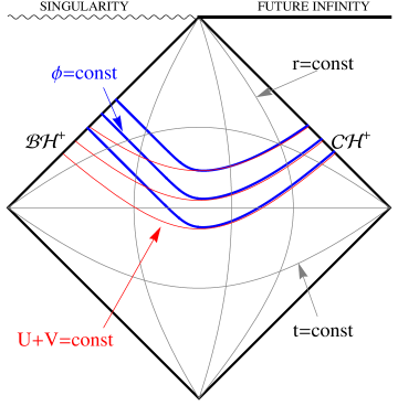
Figure 1: Contours of constant $\phi$ (thick blue) within our Hubble volume. The Penrose diagram is obtained by compactifying along the diagonal directions $U$ and $V$ using the map $x\to(1+x)/(1-x)$. For comparison, contours of constant $t$ and $r$ are shown in grey, and a constant cosmological time contour ($U+V$) shown in red. The horizons are labelled, as are the singularity and future infinity.

Figure 1 shows that the rolling of the scalar lags behind on the black hole event horizon, what is less clear is a slight lagging on the cosmological event horizon. This is more clearly seen if we plot $\phi$ as a function of $r^{*}$, as this makes the effect of the event horizons on the rolling of the scalar clearer. Figure 2 shows the profile of the scalar field as a function of $r^{*}$ at differing values of the ‘cosmological’ time parameter $\eta=(U+V)/2$. The lag due to the event horizon ($r^{*}\to-\infty$) is clearly shown here, together with a slight lag (relative to $r^{*}\approx 0$) towards the cosmological event horizon, although the $\phi$ profile becomes flat at larger $r^{*}$, as indeed it should as we expect to be close to the cosmological solution which depends only on $U+V$. (For both figure 1 and 2, the parameter values $r_{h}=1$, $r_{c}=15$ were used.)

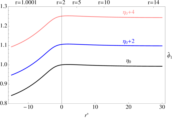
Figure 2: The profile of the perturbation of the scalar field shown as a function of $r^{*}$. The field is illustrated at three different time steps, showing the field rolling to larger $\phi$ values. This figure was produced using the values $r_{c}=15$, $r_{h}=1$, $\eta_{0}=R_{c}\sim-8.3$, and for clarity the scalar field is normalised to its value at $\eta_{0}$ and $r^{*}=0$, or alternately $t=-2R_{c}$, $r=2$: ${\hat{\phi}}_{1}=\phi_{1}/\phi_{1}(-2R_{c},2)$ where, recall, $\phi_{1}=\lambda t+\varphi$, given in (36). (For reference, $\phi_{1}(-2R_{c},2)\simeq-2.7$).

Finally, note that as $r_{h}\to 0$,

$$\phi=\phi_{0}+\sqrt{2\varepsilon}M_{p}\,\Bigl{[}\frac{2R_{c}}{r_{c}}\ln\frac{U}{R_{c}}+\ln(r+r_{c})\Bigr{]}\sim\phi_{0}-\sqrt{2\varepsilon}M_{p}\,\ln|U+V|$$ (38)

i.e., the cosmological rolling scalar solution to order ${\cal O}(\varepsilon^{1/2})$, (cf (4)). On the other hand, near the black hole event horizon,

$$\phi\sim\phi_{0}+\sqrt{2\varepsilon}M_{p}2\lambda R_{h}\ln v$$ (39)

in agreement with the linearized solutions of [30, 31].

4 Back-reaction on the black hole geometry

Clearly, since $\phi$ is regular from the black hole event horizon out to the cosmological event horizon with regular derivatives, its energy momentum is finite in this region. We can therefore compute the back-reaction on the geometry to get a consistent solution to order ${\cal O}(\varepsilon)$.

We start by comparing the first integrals of (28)

$$2\delta_{2} =2\delta_{1}+\int\frac{rV\phi_{1,V}^{2}}{R_{c}N}dV+\int\left[\frac{rV\delta_{1,VV}}{2R_{c}N}+\frac{r\delta_{1,V}}{2R_{c}N}-\frac{(rN)^{\prime}}{2N}\delta_{1,V}\right]dV+g(U)$$ (40)

$$=\delta_{1}+\int\frac{rV\phi_{1,V}^{2}}{R_{c}N}dV+\frac{rV}{2R_{c}N}\delta_{1,V}+g(U)=\delta_{1}+I_{V}+\frac{rV\delta_{1,V}}{2R_{c}N}+g$$

and (29)

$$2\delta_{2} =2\delta_{1}-\int\frac{rU\phi_{1,U}^{2}}{R_{c}N}dU-\int\left[\frac{rU\delta_{1,UU}}{2R_{c}N}+\frac{r\delta_{1,U}}{2R_{c}N}+\frac{(rN)^{\prime}}{2N}\delta_{1,U}\right]dU+f(V)$$ (41)

$$=\delta_{1}-\int\frac{rU\phi_{1,U}^{2}}{R_{c}N}dU-\frac{rU}{2R_{c}N}\delta_{1,U}+f(V)=\delta_{1}+I_{U}-\frac{rU\delta_{1,U}}{2R_{c}N}+f$$

Where $f$ and $g$ are (for now) arbitrary integration functions, and can be thought of as the perturbation of $F^{\prime}$ and $G^{\prime}$.

Substituting for $\phi_{1}$ from (31) shows that the $\phi$-integrals in (40,41) can be written as functions of $r$. For example

$$\phi_{1,V} =\frac{R_{c}}{V}\left(\lambda+N\varphi^{\prime}\right)=\frac{R_{c}}{V}\left(\lambda-H^{2}r-\frac{C}{r^{2}}\right)$$ (42)

$$\Rightarrow\quad I_{V} =\int\frac{rV\phi_{1,V}^{2}}{R_{c}N}dV=\int r\frac{dr}{dV}\left(\lambda-H^{2}r-\frac{C}{r^{2}}\right)^{2}dV+\delta g(U)$$

where the $\delta g(U)$ is added to acknowledge the fact that an integral over $V$ can have an arbitrary integration factor that is $U-$dependent, which may not be the same factor as the $r$ integral. However, since our expressions in (40) and(41) already contain integration functions, we will now without loss of generality define

$$I_{V} =\int\frac{rdr}{N^{2}}(H^{2}r+\frac{C}{r^{2}}-\lambda)^{2}$$ (43)

$$\ I_{U} =\int\frac{rdr}{N^{2}}(H^{2}r+\frac{C}{r^{2}}+\lambda)^{2}$$

and take it that the functions $f$ and $g$ are appropriately adjusted.

Next, consistency of (40,41) requires

$$U\delta_{1,U}+V\delta_{1,V}=2R_{c}\frac{\partial~{}}{\partial t}\delta_{1}=\frac{2R_{c}N}{r}\left(I_{U}-I_{V}+f-g\right)$$ (44)

which determines the general form of $\delta_{1}$ as

$$\delta_{1}=\frac{R_{c}N}{r}\left[\ln(\frac{UV}{R_{c}^{2}})(I_{U}-I_{V})+\int\frac{2f}{V}dV-\int\frac{2g}{U}dU+h(r)\right]$$ (45)

where $h(r)$ is an arbitrary integration function. Combining (40) and (41) then implicitly gives $\delta_{2}$:

$$\delta_{2}=\frac{\delta_{1}}{2}+\frac{r}{4}\frac{\partial~{}}{\partial r}\delta_{1}+\frac{I_{U}+I_{V}}{4}+\frac{f+g}{4}\;.$$ (46)

We now substitute these expressions into (2), and after some algebra, the only nonzero terms give a second order ODE for $h(r)$:

$$R_{c}\left[rN^{2}h^{\prime}\right]^{\prime}=12H^{2}r^{2}\varphi+(rN)^{\prime}\left(I_{U}+I_{V}\right)\;.$$ (47)

It proves helpful to manipulate this equation using integration by parts, and the fact that $12H^{2}r^{2}=[rN^{2}(I_{U}^{\prime}-I_{V}^{\prime})]^{\prime}/\lambda$, to find an expression for h:

$$h(r)=(I_{U}-I_{V})\frac{\varphi}{\lambda R_{c}}+h_{2}(r)+h_{3}(r)$$ (48)

where

$$h_{2}(r) =\int\frac{I_{U}}{\lambda R_{c}N}\left(\lambda+H^{2}r+\frac{C}{r^{2}}\right)+\int\frac{I_{V}}{\lambda R_{c}N}\left(\lambda-H^{2}r-\frac{C}{r^{2}}\right)$$ (49)

$$h_{3}(r) =\int\frac{1}{R_{c}rN^{2}}\int\frac{2r^{2}}{N}\left(\lambda+H^{2}r+\frac{C}{r^{2}}\right)\left(\lambda-H^{2}r-\frac{C}{r^{2}}\right)$$

Thus

$$\delta_{1}=\frac{R_{c}N}{r}\left[\frac{\phi_{1}}{\lambda R_{c}}(I_{U}-I_{V})+\int\frac{2f}{V}dV-\int\frac{2g}{U}dU+h_{2}(r)+h_{3}(r)\right]$$ (50)

It is reasonably clear that $\delta_{1}$ is regular at both event horizons, provided $f$ and $g$ are no more divergent than $V^{-1}$ or $U^{-1}$, however, we must examine regularity of $\delta_{2}$, as we still need to determine the integration functions. Inputting $\delta_{1}$ into (46) gives

$$\delta_{2}= \frac{\delta_{1}}{4}+\frac{f+g}{2}+\frac{R_{c}N^{\prime}}{4}\left(\int\frac{2f}{V}dV-\int\frac{2g}{U}dU\right)+\frac{R_{c}}{4}\left[N(h_{2}+h_{3})\right]^{\prime}$$ (51)

$$+\frac{\phi_{1}}{4\lambda}\left[N(I_{U}-I_{V})\right]^{\prime}+\frac{I_{U}}{4\lambda}\left(\lambda-H^{2}r-\frac{C}{r^{2}}\right)+\frac{I_{V}}{4\lambda}\left(\lambda+H^{2}r+\frac{C}{r^{2}}\right)$$

Clearly, the terms involving $I_{U}$, $I_{V}$ and $\delta_{1}$ are regular from the definitions of $C$ and $\lambda$, however, the residual pieces contain divergences, and we must choose $f$ and $g$ to regularise these. We will show this process in detail for the cosmological event horizon, the black hole event horizon follows the same steps.

First we identify the potentially singular behaviour of the relevant functions

$$I_{U} =\frac{a_{U}}{r-r_{c}}+b_{U}\ln|r-r_{c}|+c_{U}+J_{U}(r)$$ (52)

$$I_{V} =\frac{a_{V}}{r-r_{h}}+b_{V}\ln(r-r_{h})+c_{V}+J_{V}(r)$$

$$Nh_{3} =\frac{\alpha_{c}}{R_{c}}(r-r_{c})\ln|r-r_{c}|+\frac{\alpha_{h}}{R_{h}}(r-r_{h})\ln(r-r_{h})+N{\tilde{h}}_{3}$$

where the constants can be inferred from the appendix, $J_{U}={\cal O}(r-r_{c})$, $J_{V}={\cal O}(r-r_{h})$, and $(N{\tilde{h}}_{3})^{\prime}$ is regular. Then the singular parts appearing in (51) are:

$$\frac{\phi_{1}}{\lambda}\left[N(I_{U}-I_{V})\right]^{\prime}\Big{|}_{\rm{sing}}+R_{c}\left[N(h_{2}+h_{3})\right]^{\prime}\Big{|}_{\rm{sing}}=\frac{R_{h}}{R_{c}}b_{V}\left[\ln(r-r_{h})\right]^{2}$$ (53)

$$+\left[\alpha_{c}+2b_{U}+2c_{U}+\frac{b_{U}\phi_{1}}{\lambda R_{c}}+3a_{U}H^{2}\frac{r_{h}(r_{h}+r_{c})}{(2r_{c}+r_{h})}\right]\ln|r-r_{c}|+b_{U}\left[\ln|r-r_{c}|\right]^{2}\qquad$$

$$+\frac{R_{h}}{R_{c}}\left[\alpha_{h}+2b_{V}+2c_{V}+\frac{b_{V}\phi_{1}}{\lambda R_{h}}+3a_{V}H^{2}\frac{r_{c}(r_{h}+r_{c})}{(2r_{h}+r_{c})}\right]\ln(r-r_{h})$$

These can be cancelled by choosing $f=f_{0}+f_{1}\ln V$ and $g=g_{0}+g_{1}\ln U$, where the constants $f_{i}$ are chosen to make $\delta_{2}$ regular at $r_{c}$, and the $g_{i}$ from regularity at $r_{h}$. For example, as $r\to r_{c}$,

$$V\sim(2r_{c}+r_{h})U\left(\frac{r_{h}-r_{c}}{2r_{c}+r_{h}}\right)^{\frac{R_{h}}{R_{c}}}(r-r_{c})$$ (54)

hence

$$2f+\int\frac{2f}{V}dV\Bigg{|}_{\rm{sing}} \sim f_{1}\left(\ln V\right)^{2}+(f_{0}+f_{1})\ln V$$ (55)

$$\sim f_{1}\left[\ln|r-r_{c}|\right]^{2}+2f_{1}\ln U\ln|r-r_{c}|$$

$$+\Bigl{[}f_{0}+2f_{1} +\frac{2f_{1}R_{h}}{R_{c}}\ln(r_{c}-r_{h})+\frac{2f_{1}R_{N}}{R_{c}}\ln(r_{c}-r_{N})\Bigr{]}\ln|r-r_{c}|$$

Comparing this with (53), and recalling that $\phi_{1}\sim 2R_{C}\lambda\ln(U/R_{c})$, we see that

$$f_{1} = -b_{U}$$ (56)

$$f_{0} = \alpha_{c}+4b_{U}+2c_{U}+\frac{2b_{U}}{R_{c}}\left[R_{h}\ln(r_{c}-r_{h})+R_{N}\ln(r_{c}-r_{N})\right]+3a_{U}H^{2}\frac{r_{h}(r_{h}+r_{c})}{(2r_{c}+r_{h})}$$

with similar expressions for the $g_{i}$. The remaining, regular, parts of $\delta_{1}$ and $\delta_{2}$ are then expressible in terms of regular dilogarithms and logarithms, but the full expressions are rather lengthy and cumbersome.

Instead, by focussing on the event horizons, it is easiest to obtain results of most physical interest. For the cosmological event horizon, the $\{U,V\}$ coordinate system is appropriate, with the CEH being at $V=0$, and parametrized by $U$. Since $r=$ const. along the horizons, (11) gives

$$B=r_{c}^{2}\left(1-8\varepsilon\lambda^{2}R_{c}^{2}\ln|U|\right)\simeq r_{c}^{2}|U|^{-8\varepsilon\lambda^{2}R_{c}^{2}}$$ (57)

Setting $r_{h}\to 0$ gives $4\lambda^{2}R_{c}^{2}=1$, and hence $B\propto|U|^{-2\varepsilon}$, in complete agreement with the cosmological event horizon area of the pure rolling scalar solution, (3).

Of more interest however is the accretion of scalar field onto the black hole. Here, using the Kruskal $\{u,v\}$ system and (10), we get

$$B=r_{h}^{2}\left(1+8\varepsilon\lambda^{2}R_{h}^{2}\ln v\right)\simeq r_{h}^{2}v^{8\varepsilon\lambda^{2}R_{h}^{2}}$$ (58)

In other words, the event horizon creeps out very slowly. We can compare this with an order of magnitude estimate based on naive physical notions of mass and energy flow, [30, 31]. The flow of energy into the black hole should be governed by the difference of the energy momentum tensor from being null, $T^{0}_{0}-T^{r}_{r}$, which is of order ${\dot{\phi}}^{2}\sim W^{\prime 2}/H^{2}\sim\varepsilon H^{2}/\kappa$. Integrating this over the black hole event horizon gives $\kappa\delta{\dot{M}}\sim r_{h}^{2}\varepsilon H^{2}$, or using the relation between horizon radius and mass: $\delta A\sim r_{h}^{3}\varepsilon H^{2}\delta t$. Of course, we should be careful of using a time coordinate near the black hole event horizon, as $t\sim 2r_{h}\ln v+\ln(r-r_{h})$ is singular, however, in the spirit of this heuristic argument, we can identify $\delta t\sim 2r_{h}\delta(\ln v)$, which gives $\delta A\sim A\varepsilon(\delta\ln v)r_{h}^{2}/r_{c}^{2}$, in qualitative agreement with (58).

For an astrophysical black hole, this accretion rate is glacially slow, and far outweighed by the local environment, in which the accretion disc far outweighs local interstellar matter, let alone this cosmologically coasting scalar. However, the fact that naive local estimates of the back-reaction of accretion of scalar matter in this set-up are fully backed up by this analytic calculation, valid in the full region between the black hole and cosmological event horizons, means we should have confidence in these physically motivated techniques.

To illustrate the effect of the rolling of the scalar, in figure 3 we show the effect on the event horizon areas; for the purpose of illustration choosing $\varepsilon=0.1$, and the rather artificial initial values of $r_{c}=2$, $r_{h}=1$. Both horizons grow during the Hubble time, although the cosmological event horizon has a larger relative growth of c. 22%, as opposed to approximately 13% for the black hole event horizon.

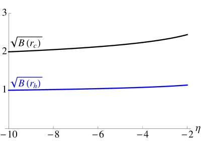
Figure 3: A plot of the variation of the event horizon areas for the initial choice of $r_{c}=2,r_{h}=1,\varepsilon=0.1$.

5 Discussion

In this paper, we have shown how to couple a slowly rolling scalar field to a black hole. We first set up the most general metric describing the physical set-up – an SO(3) symmetric geometry with dependence on both “time” and “radial distance”. This geometry is most naturally described in light-cone coordinates, which elucidate the integrable nature of the vacuum equations, and also lend themselves to an accurate determination of the black hole event horizon. Writing down the equations of motion reveals that if the potential is not too steep, the scalar field evolution will be slow, and the equations of motion can be solved perturbatively in the dynamics of the scalar field.

It is worth emphasising that although we perform an expansion in the dynamics of the scalar field, the solutions we find are exact across the the full radial range from the black hole to cosmological event horizons, and are not in any sense perturbative in the spatial (radial) coordinate. Not only do we correctly identify what the dynamical dependence is, we are able to correctly identify the cosmological evolution (and hence cosmological time) far from the black hole, as well as how the scalar field drives this expansion, and how it is dragged by the black hole. For example, we can apply these results to black holes whose event horizon constitutes a significant fraction of the Hubble volume. These black holes accrete at a similar rate to the increase in area of the cosmological event horizon.

It is interesting to compare the accretion rate of the black hole to the evaporation rate, to see whether black holes, or radiation, will dominate the final state of the universe. The black hole evaporation rate is inversely proportional to the area of its event horizon: ${\dot{M}}_{H}\sim 10^{-4}\hbar/r_{h}^{2}$, whereas the accretion rate is proportional to horizon area: $G\delta M\sim\varepsilon cH^{2}r_{h}^{2}\delta t$. Thus in order for evaporation to dominate, the horizon radius of the black hole would have to satisfy

$$r_{h}\lesssim 0.1\varepsilon^{-1/4}\left[\frac{\hbar G}{cH^{2}}\right]^{1/4}\sim 5\times 10^{-6}\varepsilon^{-1/4}{\rm m}$$ (59)

Since $\varepsilon\sim 1+w$, where $w$ is the equation of state for the dark energy, in order for astrophysical black holes to preferentially evaporate, we would require an equation of state fine tuned to approximately $|1+w|\leq{\cal O}(10^{-36})$!

We should point out that while we have a time dependent scalar field in a time dependent cosmological black hole background, this should not be viewed as a violation of the no hair theorems. The solution corresponds to a rolling cosmological scalar field in which there is a black hole, and the rolling of the scalar adjusts to its presence. The scalar does roll in the vicinity of the black hole, although it lags behind the cosmological evolution, in the sense that the constant $\phi$ contours lie in front of the constant $\eta$ contours in figure 1. However, the black hole does not have any scalar charge – there is no 1-parameter solution for $\phi$ in the black hole background. The solution (31) is not the most general solution, there will be wave like fluctuations around this background, but we have not been able to find a family of solutions with space-like dependence, which would be a signature of a scalar charge on the black hole. Thus, our results should be viewed as a way of reconciling the “no hair” intuition with more general time dependent situations.

Finally, to our knowledge, this is the first analytic procedure for finding a non-singular accreting black hole space-time from first principles (i.e. without making assumptions as to the form of the metric or solution) that results from consideration of a physically realistic matter system with physically motivated symmetries and boundary conditions. The results apply to a general potential, and only require that the scalar field is slowly rolling. As such, they represent a testing ground for investigation of black hole phenomena in the time dependent regime.

Appendix A Appendix: Some useful identities

Here we list some simple identities which are nonetheless very useful in manipulation of expressions throughout the paper.

First, we write the roots of the Schwarzschild potential as $r_{i}$ ($r_{N}<0\leq r_{h}<r_{c}$) so that

$$N(r)=-\frac{H^{2}}{r}(r-r_{c})(r-r_{h})(r-r_{N})$$ (60)

It is then simple to note the following identities:

$$r_{c}+r_{h}+r_{N} =0$$ (61)

$$r_{c}^{2}+r_{h}^{2}+r_{c}r_{h} =-r_{c}r_{h}-r_{c}r_{N}-r_{h}r_{N}=H^{-2}$$

$$r_{c}r_{h}r_{N}H^{2} =-2GM$$

We have also defined

$$R_{i}=\frac{1}{N^{\prime}(r_{i})}=\frac{r_{i}}{(1-3H^{2}r_{i}^{2})}$$ (62)

which satisfy a similar identity to the $r_{i}$

$$R_{c}+R_{h}+R_{N}=0$$ (63)

In addition, although we do not make use of the explicit forms of $I_{U}$ and $I_{V}$, we note here their form for the constants used in determining $f$ and $g$

$$I_{U} = -\frac{4r_{c}R_{c}^{2}\lambda^{2}}{(r-r_{c})}-\frac{r_{N}r_{h}^{2}R_{c}^{2}\lambda^{2}}{(r-r_{N})}+4R_{c}^{2}\lambda^{2}H^{2}(2r_{c}^{3}+r_{h}^{3})\ln|r-r_{c}|+\frac{r_{c}^{2}r_{h}^{2}}{(r_{c}^{2}+r_{h}^{2})^{2}}\ln r$$ (64)

$$+\frac{r_{h}}{r_{c}^{2}}\lambda^{2}R_{c}^{2}H^{2}(4r_{c}^{4}+2r_{c}^{3}r_{h}+3r_{c}^{2}r_{h}^{2}+5r_{c}r_{h}^{3}+r_{h}^{4})\ln(r-r_{N})$$

$$I_{V} = -\frac{4r_{h}R_{h}^{2}\lambda^{2}}{(r-r_{h})}-\frac{r_{N}r_{c}^{2}R_{h}^{2}\lambda^{2}}{(r-r_{N})}+4R_{h}^{2}\lambda^{2}H^{2}(2r_{h}^{3}+r_{c}^{3})\ln(r-r_{h})+\frac{r_{c}^{2}r_{h}^{2}}{(r_{c}^{2}+r_{h}^{2})^{2}}\ln r$$ (65)

$$+\frac{r_{c}}{r_{h}^{2}}\lambda^{2}R_{h}^{2}H^{2}(4r_{h}^{4}+2r_{h}^{3}r_{c}+3r_{c}^{2}r_{h}^{2}+5r_{h}r_{c}^{3}+r_{c}^{4})\ln(r-r_{N})$$

References

• [1] R. Ruffini and J. A. Wheeler, Physics Today 24, 30 (1971).
• [2] B. Carter, Phys. Rev. Lett.  26, 331 (1971).
• [3] J. D. Bekenstein, Phys. Rev. D 5, 1239 (1972).
• [4] S. L. Adler and R. B. Pearson, Phys. Rev. D 18, 2798 (1978).
• [5] J. D. Bekenstein, Phys. Rev. D 51, 6608 (1995).
• [6] A. E. Mayo and J. D. Bekenstein, Phys. Rev. D 54, 5059 (1996) [gr-qc/9602057].
• [7] P. Bizon, Phys. Rev. Lett.  64, 2844 (1990).
• [8] A. Achucarro, R. Gregory and K. Kuijken, Phys. Rev. D 52, 5729 (1995) [gr-qc/9505039].
• [9] T. Torii, K. Maeda and M. Narita, Phys. Rev. D 64, 044007 (2001).
• [10] K. G. Zloshchastiev, Phys. Rev. Lett.  94, 121101 (2005) [hep-th/0408163].
• [11] R. R. Caldwell, R. Dave and P. J. Steinhardt, Phys. Rev. Lett.  80, 1582 (1998) [astro-ph/9708069].
• [12] E. J. Copeland, M. Sami and S. Tsujikawa, Int. J. Mod. Phys. D 15, 1753 (2006) [hep-th/0603057].
• [13] S. J. Poletti and D. L. Wiltshire, Phys. Rev. D 50, 7260 (1994) [Erratum-ibid. D 52, 3753 (1995)] [gr-qc/9407021].
• [14] J. D. Barrow, Phys. Rev. D 46, R3227 (1992) [Erratum-ibid. D 47, 1730 (1993)].
• [15] G. C. McVittie, Mon. Not. Roy. Astron. Soc.  93, 325 (1933).
• [16] N. Kaloper, M. Kleban and D. Martin, Phys. Rev. D 81, 104044 (2010) [arXiv:1003.4777 [hep-th]].
• [17] J. Sultana and C. C. Dyer, Gen. Rel. Grav.  37, 1347 (2005).
• [18] V. Faraoni and A. Jacques, Phys. Rev. D 76, 063510 (2007) [arXiv:0707.1350 [gr-qc]].
• [19] M. Carrera and D. Giulini, Phys. Rev. D 81, 043521 (2010) [arXiv:0908.3101 [gr-qc]].
• [20] B. J. Carr and S. W. Hawking, Mon. Not. Roy. Astron. Soc.  168, 399 (1974).
• [21] D. N. C. Lin, B. J. Carr and S. M. Fall, Mon. Not. Roy. Astron. Soc.  177, 51 (1976).
• [22] G. V. Bicknell and R. N. Henriksen, Ap. J. 219, 1043 (1978)
• [23] H. Maeda, T. Harada and B. J. Carr, Phys. Rev. D 77, 024023 (2008) [arXiv:0707.0530 [gr-qc]].
T. Harada, H. Maeda and B. J. Carr, Phys. Rev. D 77, 024022 (2008) [arXiv:0707.0528 [gr-qc]].
• [24] T. Harada, C. Goymer and B. J. Carr, Phys. Rev. D 66, 104023 (2002) [astro-ph/0112563].
• [25] B. J. Carr, T. Harada and H. Maeda, Class. Quant. Grav.  27, 183101 (2010) [arXiv:1003.3324 [gr-qc]].
• [26] P. Vaidya, Proc. Indian Acad. Sci. A 33, 264 (1951).
• [27] V. Husain, E. A. Martinez and D. Nunez, Phys. Rev. D 50, 3783 (1994) [gr-qc/9402021].
• [28] O. A. Fonarev, Class. Quant. Grav.  12, 1739 (1995) [gr-qc/9409020].
• [29] M. Carrera and D. Giulini, arXiv:0810.2712 [gr-qc].
• [30] T. Jacobson, Phys. Rev. Lett.  83, 2699 (1999) [astro-ph/9905303].
• [31] A. V. Frolov and L. Kofman, JCAP 0305, 009 (2003) [hep-th/0212327].
• [32] P. Bowcock, C. Charmousis and R. Gregory, Class. Quant. Grav.  17, 4745 (2000) [hep-th/0007177].
• [33] C. Charmousis and R. Gregory, Class. Quant. Grav.  21, 527 (2004) [gr-qc/0306069].