Merging of Dirac points and Floquet topological transitions in AC driven graphene

Abstract

We investigate the effect of an in-plane AC electric field coupled to electrons in the honeycomb lattice and show that it can be used to manipulate the Dirac points of the electronic structure. We find that the position of the Dirac points can be controlled by the amplitude and the polarization of the field for high frequency drivings, providing a new platform to achieve their merging, a topological transition which has not been observed yet in electronic systems. Importantly, for lower frequencies we find that the multi-photon absorptions and emissions processes yield the creation of additional pairs of Dirac points. This provides an additional method to achieve the merging transition by just tuning the frequency of the driving. Our approach, based on Floquet formalism, is neither restricted to specific choice of amplitude or polarization of the field, nor to a low energy approximation for the Hamiltonian.

I Introduction

Since the recent discovery of topological insulatorshasan10 ; qi11 , the search for topological transitions in condensed matter has become a priority task. In particular, the prediction and the observation of a new topological order, namely the $\mathbb{Z}_{2}$ topological orderkane_z2_2005 ; bernevig06 ; konig07 , has stimulated a great interest in the scientific community. Graphene, a two-dimensional carbon-based crystal, is a wonderful platform for investigating topological transitions. It is a semi-metal, whose band structure of the $p_{z}$ orbitals consists in two bands that touch linearly at the Fermi level at two inequivalent points of the Brillouin zonecastrorevue09 . This peculiar structure gives rise to massless Dirac-like low energy excitations.

On the other hand, several ideas to induce topological states of matter by means of time periodic external potentials have been proposedinoue10 ; linder11 ; gu11 ; Kitagawa_Graphene ; AGL_GP_Floquet ; cayssol , and recently observed in temporal modulated photonic crystals rechtsman13 . This approach renews considerably the possibilities of inducing new topological phases. Remarkably in graphene, a different topological transition between a Dirac semi-metallic phase and an insulating phase, can also be achieved by merging the pair of Dirac points (PDP)dietl08 ; guinea08 ; pereira_strain . The resulting insulating phase is not a $\mathbb{Z}_{2}$ topological phase, but may nevertheless host zero-energy edge states whose topological origin is well understood in terms of a one-dimensional bulk winding number, namely the Zak phasezak ; hatsugai02 ; delplace_zak . The search for this transition has stimulated experimental efforts beyond the solid state community: The merging of the Dirac points, as well as the emergence of zero-energy edge states have been recently observed in anisotropic traps of cold atomstarruell12 ; lim12 and in microwave tight-binding analogue experiments of a honeycomb latticerechtsman12 ; mortessagne13 . However, the merging transition has not been observed yet in electronic systems. In particular its achievement in graphene itselfmontambaux09 , by means of mechanical manipulations like stretching, is unfortunately out of reach, because the graphene sheet would be destroyed far before the expected transitionpereira_strain .

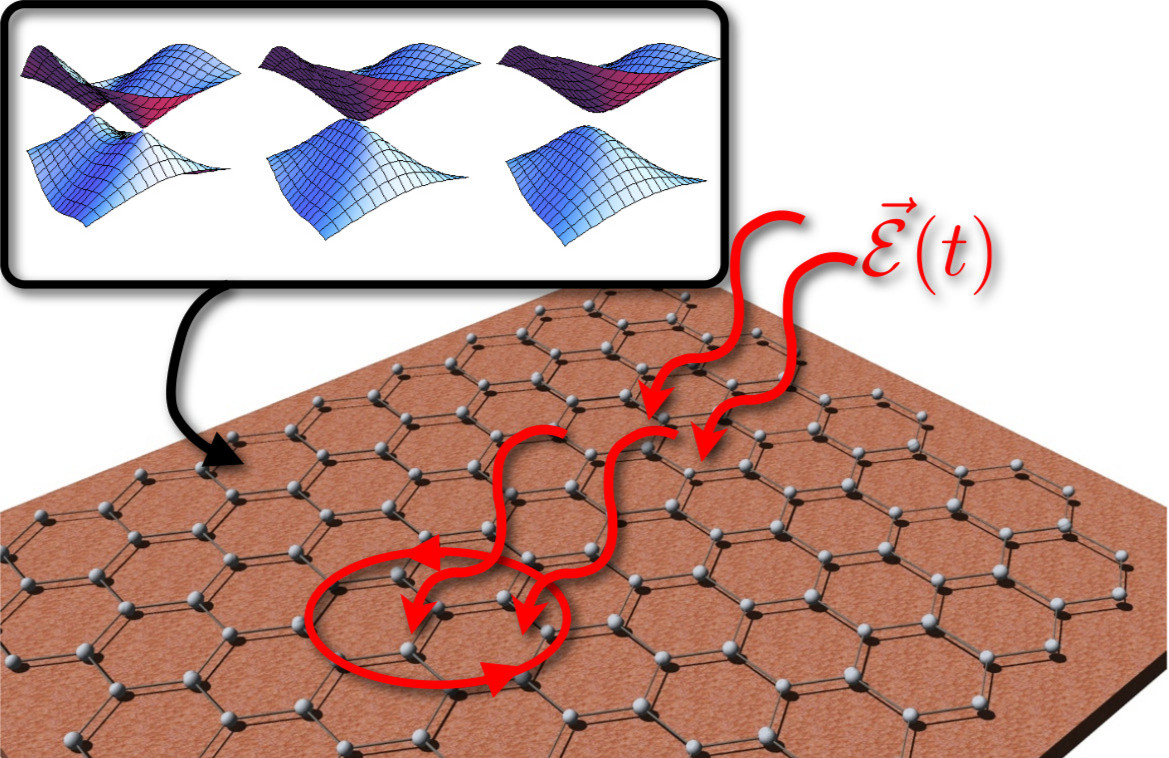
Figure 1: Honeycomb lattice irradiated by an AC electric field with arbitrary polarization. The inset shows the merging of the Dirac points induced by the external field.

In the present work, we propose an alternative to mechanical distortions to achieve the merging transition in the honeycomb lattice. In particular, we show that an AC electric field can drive the topological merging transition, or inversely induce the creation of new Dirac points. This mechanism is different to the ones usually studied in previous works dealing with Floquet topological insulators and summarized in cayssol . More precisely, we demonstrate that in the high frequency regime, the AC field acts similarly to a mechanical strain, and therefore allows for the manipulation of the Dirac points, their annihilation and their creation in a controllable way. Furthermore, the AC field is able to induce the localization of the electrons in specific directions by aligning the Dirac points, which marks another topological transition between two insulating or two semi-metallic phases. Our analysis, when restricted to linear polarization and high frequency regime, agrees with the results obtained in shaken optical latticeskoghee12 . In addition, we also consider different field polarizations and finite frequency effects. Importantly, at lower frequencies, we find that the coupling between the Floquet bands, that characterize the properties of the driven system, gives rise to out-of-equilibrium phases with no analogue in the static system in which multiple PDP emerge. Our approach does not rely neither on low energy models nor on approximations valid just close to resonance (as the rotating wave approximation)Maria ; gu11 ; linder11 , but takes into account the full lattice model together with arbitrary field amplitudes and phase polarizations. This allows us to keep track of the relative position between the Dirac points and thus properly describe their annihilation or creation.

II Floquet theory on the honeycomb lattice

The Hamiltonian of a $T$-periodic driven system fulfills $H\left(\tau+T\right)=H\left(\tau\right)$, and its eigenvectors can then be written in the Floquet form: $|\psi\left(\tau\right)\rangle=e^{-i\epsilon\tau}|\Phi\left(\tau\right)\rangle$ ($\hbar=1$), being $\epsilon$ the quasi-energy, and $|\Phi\left(\tau\right)\rangle=|\Phi\left(\tau+T\right)\rangle$ the Floquet stategloria04 ; AGL_GP_Floquet . This ansatz, consequence of the time translation invariance, maps the time-dependent Schrödinger equation to the eigenvalue equation $\mathcal{H}\left(t\right)|\Phi\left(\tau\right)\rangle=\epsilon|\Phi\left(\tau\right)\rangle$, in which the quasi-energies and the Floquet states are the eigenvalues and eigenvectors of the Floquet operator $\mathcal{H}\left(\tau\right)\equiv H\left(\tau\right)-i\partial_{\tau}$, respectively. In order to deal with the time dependence of the Floquet operator $\mathcal{H}\left(\tau\right)$, it is useful to introduce the Sambe space, which consists in a composed Hilbert space, where the basis states are time-independentsambe73 . In this space, the quasi-energies are given by (see AGL_GP_Floquet and Appendix A):

$$\epsilon=\sum_{p,p^{\prime}}\langle\Phi_{p^{\prime}}|H_{p^{\prime}-p}|\Phi_{p}\rangle-\ \delta_{p,p^{\prime}}p\omega$$ (1)

where $H_{p^{\prime}-p}=\int_{0}^{T}\frac{d\tau}{T}e^{i\omega\tau(p^{\prime}-p)}H(\tau)$ with $\omega=2\pi/T$, and where $\Phi_{p^{(\prime)}}$ is the $p^{(\prime)}-\text{th}\in\mathbb{Z}$ Fourier component of the Floquet state. The coupling between the Floquet side-bands is encoded in the Fourier components $H_{p^{\prime}-p}$ of the Hamiltonian.

For a honeycomb lattice embedded in a periodic time-dependent in-plane electric field $\mathbf{{\cal E}}(\tau)$ (see Fig.1), the Peierls substitution leads to a time dependent Hamiltonian:

$$H(\tau,\mathbf{k})=\left(\begin{array}[]{cc}0&\rho(\tau,\mathbf{k})\\ \rho^{*}(\tau,\mathbf{k})&0\end{array}\right),$$ (2)

where $\rho(\tau,\mathbf{k})=\sum_{j}t_{j}(\tau)e^{i\mathbf{k}\cdot\mathbf{a}_{j}}$, $t_{j}(\tau)=te^{i\mathbf{d}_{j}\cdot\mathbf{A}(\tau)}$ being $t$ the nearest neighbor hopping parameter, $\mathbf{a}_{j=1,2}$ are the basis vectors of the Bravais lattice: $\mathbf{a}_{1}=\frac{a}{2}\left(3,-\sqrt{3}\right)$, $\mathbf{a}_{2}=\frac{a}{2}\left(3,\sqrt{3}\right)$, and $\mathbf{a}_{3}=a\left(0,0\right)$. The vectors joining the nearest neighbors $\mathbf{d}_{j}$ are given by $\mathbf{d}_{1}=\frac{a}{2}\left(-1,\sqrt{3}\right)$, $\mathbf{d}_{2}=\frac{a}{2}\left(-1,-\sqrt{3}\right)$, $\mathbf{d}_{3}=a\left(1,0\right)$. We consider electric fields with arbitrary amplitude and polarization, and write the vector potential as $\mathbf{A}(\tau)=(A_{x}\sin(\omega\tau),A_{y}\sin(\omega\tau+\varphi))$. The calculation of the Fourier components $H_{q=p^{\prime}-p}(\mathbf{k})$ can be performed analytically (see Appendix B) and yields:

$$H_{q}(\mathbf{k})=\left(\begin{array}[]{cc}0&\rho_{q}(\mathbf{k})\\ \rho_{-q}^{*}(\mathbf{k})&0\end{array}\right),$$ (3)

with $\rho_{q}(\mathbf{k})=\sum_{j}t_{j,q}^{F}e^{i\mathbf{k}\cdot\mathbf{a}_{j}}$, and where we have defined the time independent Floquet hoppings $t_{j,q}^{F}=tJ_{-q}({\cal A}_{j})e^{iq\Psi_{j}}$, being $J_{q}\left(x\right)$ the $q^{\text{th}}$ order Bessel function of the first kind. The dimensionless functions ${\cal A}_{j}$ and $\Psi_{j}$ encode all the information of the field configuration:

$$\begin{split}{\cal A}_{2,1}=&\frac{a}{2}\sqrt{A_{x}^{2}+3A_{y}^{2}\pm 2\sqrt{3}A_{x}A_{y}\cos\left(\varphi\right)},\\ \Psi_{2,1}=&\pm\arctan\left[\frac{\sqrt{3}A_{y}\sin\left(\varphi\right)}{A_{x}\pm\sqrt{3}A_{y}\cos\left(\varphi\right)}\right],\\ {\cal A}_{3}=&A_{x}a,\quad\Psi_{3}=0\ .\end{split}$$ (4)

As a consequence, a spatial anisotropy can be tuned by varying the polarization or the amplitude of the field. This is the key result of the present work.

For the sake of clarity, we shall first focus on the high frequency regime $\omega\gg t$. In that limit, the Floquet bands are uncoupled and the zeroth Fourier component ${\cal H}_{q=0}$ of the Floquet operator is the dominant one. Thus, Eq.1 is block-diagonal in the Fourier space, and simply consists in a collection of identical $2\times 2$ time-independent Hamiltonians separated in energy by $\omega$. The quasi-energy of a side-band $\alpha$, is then simply given by $\epsilon_{\alpha}(\mathbf{k};A_{x},A_{y},\varphi)=\pm|\rho_{q=0}(\mathbf{k};A_{x},A_{y},\varphi)|+\alpha\omega$, which shows that the quasi-energy of each Floquet band is, in the high-frequency regime, identical to the energy bands of the undriven honeycomb lattice with renormalized hopping parameters $t_{j,0}^{F}(A_{x},A_{y},\varphi)=tJ_{0}({\cal A}_{j})$.

III Manipulation of the Dirac points by the AC field: merging and localization

In this section, we analyze the fate of the Dirac points of the quasi-energy spectrum in the high frequency regime as a function of the parameters of the electric field. Note that in this regime, the renormalized hoppings $tJ_{0}({\cal A}_{j})$ are real parameters, so that the system is still time-reversal invariant for all field polarizations, and the Dirac nodes are thus well definedGDP-AQHE . A direct consequence of the AC field induced anisotropy of the hopping parameters, is to change the location of the Dirac points. The two Dirac points, related by time-reversal and inversion symmetry, move as the anisotropy is modified and merge at one of the four time-reversal (inversion) symmetric points of the Brillouin zone M_i, whenever a specific relation between the hopping parameters is fulfilled guinea08 ; montambaux09 ; merginguniv09 :

$$\begin{split}&\text{M}_{0},\quad t_{1}^{F}+t_{2}^{F}+t_{3}^{F}=0\qquad\ \text{M}_{1},\quad t_{1}^{F}=t_{2}^{F}+t_{3}^{F}\\ &\text{M}_{2},\quad t_{2}^{F}=t_{1}^{F}+t_{3}^{F}\qquad\qquad\text{M}_{3},\quad t_{3}^{F}=t_{1}^{F}+t_{2}^{F}\end{split}$$ (5)

where the index $0$ has been dropped out for clarity. The merging transition corresponds to the creation/annihilation of a PDP. At the transition, the so-called semi-Dirac dispersion relation is quadratic in one direction, but remains linear in the other one, leading to the prediction of striking properties such as an unusual temperature dependence of the specific heat and magnetic field dependence of the Landau levels merginguniv09 . Such transitions can now be achieved for specific values of amplitude $(A_{x},A_{y})$ and polarization $\varphi$ of the electric field.

The system exhibits several distinct semi-metallic and insulating phases that we now describe. Fig.2 shows a typical example of a semi-metallic/insulating phase diagram obtained in the high frequency regime when varying the amplitude and the polarization of the field (other examples are shown in the Appendix C). The creation/annihilation of a PDP at a M_i point is represented by a continuous merging line that separates a semi-metallic phase from an insulating phase. Thus, there are four different merging lines, one for each point M_i. It follows that distinct semi-metallic or insulating phases (coloured differently) may emerge when different merging lines are crossed. This distinction can be made in terms of both the points M_i and topological (winding) numbers: Each semi-metallic phase can be labeled by a point M_i where a PDP cannot be annihilated. For instance, a PDP cannot be annihilated at M₀ (green line) from the semi-metallic phase $\text{SM}_{0}$ (which is the one connected to the undriven graphene phase). The reason is that all the hopping parameters in the $\text{SM}_{0}$ phase have the same sign, so that the merging at $\text{M}_{0}$ would require first a change in sign of any of them, and according to Eq.5, it would fulfill the merging conditions at other M_i≠0 point. Therefore, one can distinguish four semi-metallic phases, denoted as $\text{SM}_{i}$, one for each $\text{M}_{i}$ point where the merging transition cannot occur. In addition, two winding numbers can be introduced to characterize the topology of these four semi-metallic phases. Indeed, the topological properties of out-of-equilibrium Floquet systems can be characterized in a similar way to those of static systems (see for instance Ref.AGL_GP_Floquet ). The first one is the quantized Berry phase around a Dirac point, giving rise to a topological charge $\frac{1}{2\pi}\oint d\mathbf{k}\cdot\nabla_{\mathbf{k}}\theta_{\mathbf{k}}=\pm 1$ assigned to each Dirac point, where $\theta_{\mathbf{k}}=\text{arg}\rho(\mathbf{k})$ is the polar angle parameterizing the Bloch sphere. The two Dirac points of graphene carry opposite topological charges that annihilate at the merging transition montambaux09 . Besides, the topological transition is accompanied with a change of a second winding number, the Berry phase evaluated across a reduced one-dimensional Brillouin zone, namely the Zak phase $Z=\frac{1}{2\pi}\int_{-\mathbf{G}/2}^{\mathbf{G}/2}\left\{d\mathbf{k}\cdot\nabla_{\mathbf{k}}\theta_{\mathbf{k}}\right\}$, where $\mathbf{G}$ is a vector of the reciprocal lattice. Chiral symmetry guaranties integer values of the Zak phase hatsugai02 which depend on the direction in the reciprocal space. This reflects the edge orientations dependence for the density of zero-energy edge modes delplace_zak . Thus, the four semi-metallic phases differ by the set of values the Zak phase takes for all directions in the reciprocal space, and therefore by the range of existence in $k$-space of edge zero-energy modes for a given edge orientation.

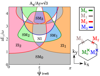
Figure 2: Semi-metallic (SM) / insulating (I) phase diagram ($\varphi,aE_{y}/\omega$) in the high frequency regime for fixed $A_{x}/A_{y}=\sqrt{3}$, with $a$ the lattice spacing. NI (ZI) denotes a normal (Zak) insulating phase. The different phases, which are represented in different colors, are separated by four distinct merging lines corresponding to the four M_i points of the first Brillouin zone (shown on the right) where a PDP can be created/annihilated.

Similarly, different insulating phases can be distinguished as well by the set of values the Zak phase takes in all possible directions, even though a PDP can, in principle, be created at any of the four points M_i. We find one normal insulating (NI) phase for which the Zak phase is zero in every directions (meaning the absence of zero-energy edge states), and, for polarizations different than $\varphi=\pi/2$, two Zak insulating phases for which the Zak phase is non zero in different directions. The Zak insulating phases reflect, in 2D, the underlying non-trivial topology expected for a BDI symmetry class in 1Dschnyder_classification_2009 .

Interestingly, the phase diagrams show multiple crossings between the merging lines, meaning that a PDP can be created and annihilated simultaneously at two different $\text{M}_{i}$ points. Following Eq.5, such crossings actually imply the vanishing of one of the three hopping parameters $t_{j}^{F}$, what directly induces localization of the electrons in the direction $\mathbf{d}_{j}$. This striking feature corresponds to a transition between two insulating or two semi-metallic phases. At the transition, the gap closes along lines parallel to the $\mathbf{d}_{j}$ direction that passes through the two distinct merging points. Unlike a single merging transition, it follows that the dispersion relation is flat along the $\mathbf{d}_{j}$ direction but remains linear in the other one, as shown in Fig.3 (c). At the transition, the system is then reduced to an array of uncoupled one-dimensional chains, hosting one-dimensional massless Dirac fermions. Remarkably, for phase polarization $\varphi=\pi/2$, the merging at $M_{1}$ and $M_{2}$ is always coincident. This gives rise to critical localization lines that separate two SM phases as shown in Fig.3. At the transition between two semi-metallic phases, the topological charges assigned to the Dirac points change sign (see Fig.3 (b) and (d)). In that sense, the localization (or double merging) transition is also a topological transition. Finally, we report that the phase diagram for polarization $\varphi=\pi/2$ also exhibits crossings between the four merging lines simultaneously. At such critical points, all the hopping parameters $t_{j}^{F}$ vanish and the quasi-energy of each side-band is perfectly flat which leads to full charge localization in all directions.

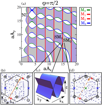
Figure 3: (a) Semi-metallic (SM) / insulating (I) phase diagram in the high frequency regime for $\varphi=\pi/2$, where only three phases appear, due to the overlap between the M₁ and M₂ merging lines. (c) This overlap gives rise to localization lines separating two semi-metallic phases. At the transition between these two semi-metallic phases, the topological charges assigned to each Dirac point change sign ((b) and (d)). This topological transition goes together with a change of the value of the Zak phase, which is $1$ ($0$) in the SM₃ (SM₀) phase along the path represented by a full (dashed) arrow.

IV Multi side-bands effects and emergence of additional Dirac points

Although the merging transition in the high frequency regime is simple to describe, it might be difficult to achieve experimentally in graphene, since it requires high field amplitudes which also would involve heating effects. For that reason, we now investigate the effect of a frequency decrease and show that the merging transition may also be achieved by varying the frequency, and thus requires smaller intensities of the AC field. Importantly, besides being more relevant experimentally, it turns out that such a regime is particularly interesting since it allows us to engineer additional Dirac points.

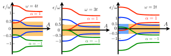
Figure 4: Sketch of the first uncoupled side-bands $\alpha=0,\pm 1$ as a function of a parameter (for instance the field amplitude), for different driving frequencies. The colored area highlight the range where the side-bands are inverted.

The high frequency regime holds as long as the frequency is larger than the bandwidth of the undriven system, namely, $\omega>6t$. For lower frequencies ($3t<\omega\lesssim 6t$) the coupling between the Floquet side-bands becomes relevant, and the high frequency effective theory is not accurate. Besides, unless the polarization of the field is linear, the couplings break time reversal symmetry and will therefore open a gap at the Dirac points. In the following, we therefore restrict our analysis to linearly polarized fields only, although our formalism remains valid for any phase polarization.

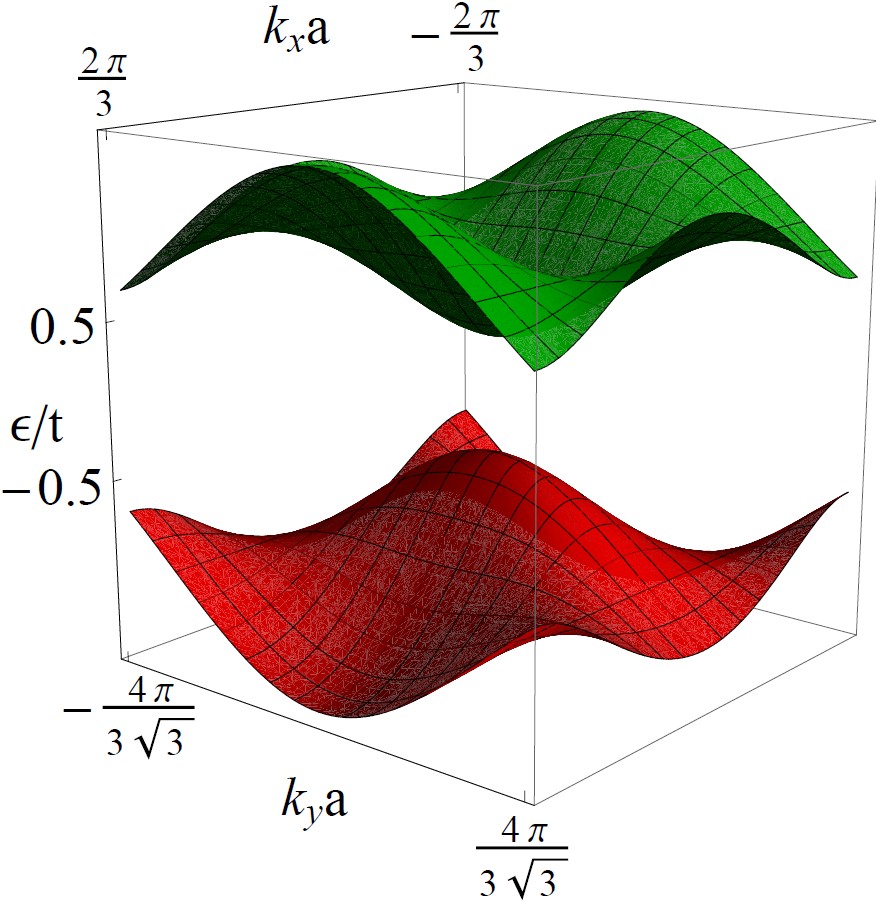
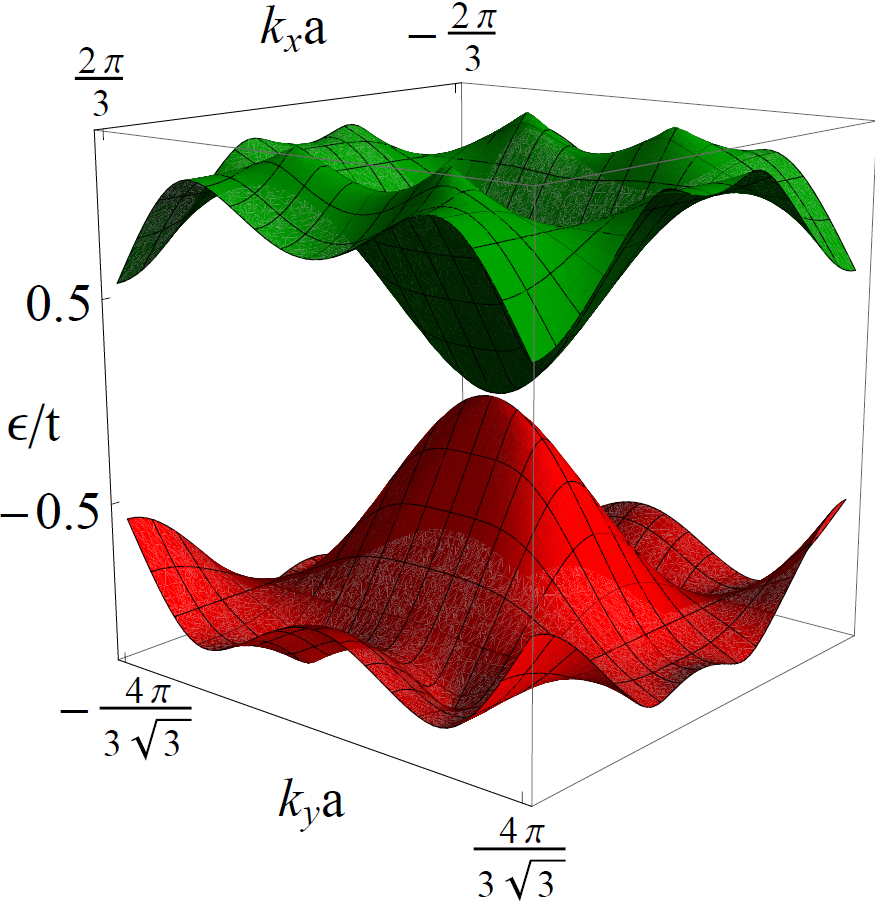
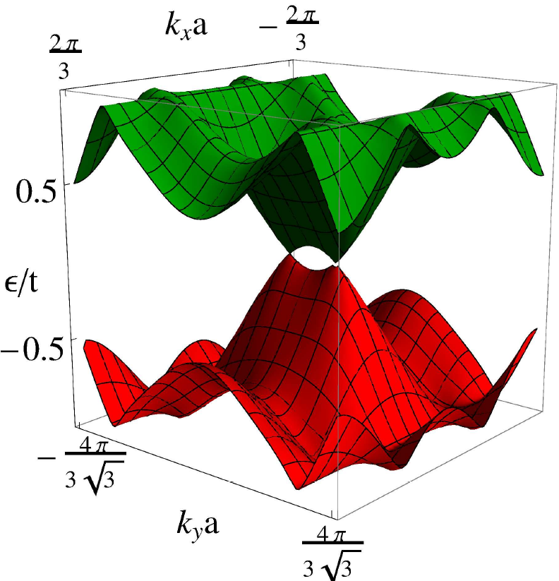
Figure 5: Quasi-energy spectra for $A_{y}=3.6$, $A_{x}=0$ and $\varphi=0$ with (top, left) $\omega=10t$, (top, right) $\omega=2.5t$, (bottom, left) $\omega=2.1t$ and (bottom, right) $\omega=1.5t$.

As illustrated in Fig.4, the Floquet side-bands overlap as the frequency is decreased. This yields new couplings which can now include the absorption or the emission of photons. At around about $\omega=3t$, the (uncoupled) side-bands $\alpha=+1$ and $\alpha=-1$ are expected to touch at $\epsilon=0$ for vanishing amplitude of the field, giving rise to a new crossing at the $\text{M}_{0}$ point. This new crossing corresponds to a band inversion, in which the symmetries of the conduction band and the valence band are exchanged. As the high frequency approximation fails to describe this situation, the Floquet operator is now diagonalized numerically.

For more concreteness, we fix the system in a normal insulating phase in the high frequency regime by choosing suitable field amplitudes (Fig.5, top, left). Then, we decrease the frequency such that the side-bands $\alpha=+1$ and $\alpha=-1$ cross. This leads to the appearance of a PDP at the center of the Brillouin zone $\text{M}_{0}$ for $\omega=2.5t$ with the typical semi-Dirac dispersion relation (quadratic in one direction and linear in the other one, as it is shown in Fig.5, top, right). When the frequency is further decreased, the two Dirac points move away to each other while the rest of the bands bend (Fig.5, bottom, left). A larger decrease of frequency makes the bands close the gap once again at the $\text{M}_{3}$ point of the FBZ. This creates a second PDP with the same typical semi-Dirac shape, which move away as the frequency is lowered, as it is shown in Fig.5, bottom, right. Then, for lower frequencies the band structure now owns four Dirac points at the same quasi-energy. Therefore, the driving field offers not only the opportunity to manipulate the Dirac points, but also to create new ones and observe the merging transition by just tuning the frequency of the AC field.

V Discussion

We have shown that the merging of the Dirac points in the honeycomb lattice can be driven in a controllable way by an AC electric field. We have obtained rich phase diagrams in which distinct topological semi-metallic and insulating phases emerge. At high frequency, $\omega\gg t$, the behavior is easily described by an effective Floquet operator, equivalent to the Hamiltonian of undriven graphene, but with renormalized hoppings tuned by the field amplitude and the phase polarization. The resulting phases reflect interesting topological features, and the critical lines in which pairs of Dirac points are created and annihilated simultaneously show unexpected localization properties for which electrons behave relativistically in one direction, while they are localized in the other one.

Importantly, we also proved that out of the high frequency regime ($\omega\gtrsim t$), and for linearly polarized fields, a change in frequency can drive a novel transition with the emergence of new pairs of Dirac points, although it does not necessarily correspond to a transition between an insulating and a semi-metallic phase. This new transition lies on multi-side-bands couplings, or in other words, multi-photon assisted transitions. The resulting new semi-metallic phase with four Dirac points can clearly be distinguished from the one with two Dirac points by various transport measurements. For instance, a Hall conductance measurement would provide a direct signature of the two additional Dirac points, since each valley brings a contribution $e^{2}/h(1/2+n)$ to the total transverse conductivity, where $n$ is the number of Landau levels. The conductivity measurements would be accomplished by considering the Floquet sum rule obtained in Ref.steady , due to the far from equilibrium situation of the setup at intermediate frequencies $\omega\sim t$. We also notice that for samples of the size of or smaller than the wave length ($\approx 1$ micron), the effect of the magnetic field of the irradiation can be ignored.

For the realization in graphene, the high frequency regime requires field frequencies in the near ultraviolet and field amplitudes at least of the order $\approx 3.4\text{V}\textrm{\AA}^{-1}$ Experiment1 ; Experiment2 ; Experiment3 . The energy corresponding to this electric field is about half the ionization energy of carbon atoms. However, real graphene also possesses $s$-orbitals which can be affected by such a high frequency field. Thus, in order to achieve the high frequency regime, a frequency larger than the actual band width of the graphene bands must be considered. In addition, for fields of both high frequency and high amplitude, the heating of the sample will certainly be an issue because of the dissipative processes due to phonons and electron-electron scattering. One way to partially avoid these issues can be the use of alternative platforms with similar properties, such as artificial grapheneArtificial-graphene . This would help in two different ways: The increase of the lattice parameter allows one to consider lower frequencies and thus lower the field intensities, while in addition, the contribution of the $s$-orbitals would vanish. Finally, we expect that the results obtained in the lower frequency regime ($\omega\gtrsim t$) to be more easily achievable in real graphene, if only because the undesirable heating of the sample will be reduced. Furthermore, we stress that this regime allows one not only to manipulate the Dirac points but also to create new ones just by tuning the frequency.

Acknowledgments: The authors would like to thank Janos Asboth, Jian Li, Markus Büttiker, Hector Ochoa, Alexey Kuzmenko and F. Koppens for inspiring discussions. P. D. was supported by the European Marie Curie ITN NanoCTM. Á. Gómez-León acknowledges JAE program. Á. G. L. and G. P. acknowledge MAT 2011-24331 and ITN, grant 234970 (EU) for financial support.

Appendix A Appendix A: Floquet-Bloch theory

Crystals coupled to in-plane AC electric fields have lattice and time translation invariance: $H\left(\mathbf{x}+\mathbf{a}_{i},\tau+T\right)=H\left(\mathbf{x}+\mathbf{a}_{i},\tau\right)=H\left(\mathbf{x},\tau+T\right)$, being $\mathbf{a}_{i}$ the lattice vectors and $T=2\pi/\omega$ a period of the driving field. Thus, one can assume solutions in Floquet-Bloch form $|\Psi_{\alpha,\mathbf{k}}\left(\mathbf{x},\tau\right)\rangle=e^{i\mathbf{k}\cdot\mathbf{x}-i\epsilon_{\alpha,\mathbf{k}}\tau}|u_{\alpha,\mathbf{k}}\left(\mathbf{x},\tau\right)\rangle$, where $\epsilon_{\alpha,\mathbf{k}}$ is the quasi-energy for the $\alpha$ Floquet state, and $\mathbf{k}$ the wave-vector. The Floquet-Bloch states $|u_{\alpha,\mathbf{k}}\left(\mathbf{x},\tau\right)\rangle$ are periodic in both $\mathbf{x}$ and $\tau$, and fulfill the Floquet eigenvalue equation:

$$\mathcal{H}\left(\tau,\mathbf{k}\right)|u_{\alpha,\mathbf{k}}\rangle = \epsilon_{\alpha,\mathbf{k}}|u_{\alpha,\mathbf{k}}\rangle,$$ (6)

$$\mathcal{H}\left(\tau,\mathbf{k}\right) \equiv e^{-i\mathbf{k}\cdot\mathbf{x}}\left(H\left(\tau\right)-i\partial_{\tau}\right)e^{i\mathbf{k}\cdot\mathbf{x}}$$ (7)

$$= H_{\mathbf{k}}\left(\tau\right)-i\partial_{\tau}$$

where $\mathcal{H}\left(\mathbf{k},\tau\right)$ is the Floquet operator. The time dependent Hamiltonian is obtained through the Peierls substitution in the tight binding model, leading to the time dependent hoppings $t_{j}^{\alpha,\beta}\left(\tau\right)=t_{j}^{\alpha,\beta}e^{i\mathbf{A}\left(\tau\right)\cdot\mathbf{d}_{j}}$, and to the time dependent Hamiltonian:

$$H\left(\tau,\mathbf{k}\right)=\sum_{\alpha,\beta}\sum_{j}c\left(\tau\right)_{\alpha,\mathbf{k}}^{\dagger}c\left(\tau\right)_{\beta,\mathbf{k}}t_{j}^{\alpha,\beta}\left(\tau\right)e^{i\mathbf{k}\cdot\mathbf{a}_{j}},$$ (8)

where we have included the sub-lattice indexes $\alpha$, $\beta$, and the time dependent annihilation and creation operators of Floquet-Bloch states. Due to its time periodicity, we expand in Fourier series $c\left(\tau\right)_{\alpha,\mathbf{k}}$ and $c\left(\tau\right)_{\alpha,\mathbf{k}}^{\dagger}$:

$$H\left(\tau,\mathbf{k}\right) =\sum_{\alpha,\beta}\sum_{p,p^{\prime}}\sum_{j}t_{j}^{\alpha,\beta}\left(\tau\right)e^{i\omega\tau\left(p^{\prime}-p\right)}e^{i\mathbf{k}\cdot\mathbf{a}_{j}}c_{\alpha,\mathbf{k},p^{\prime}}^{\dagger}c_{\beta,\mathbf{k},p}\ .$$ (9)

Eq.9 gives a description of the time dependent Hamiltonian in terms of the time independent operators $\left\{c_{\alpha,\mathbf{k},p},c_{\alpha,\mathbf{k},p}^{\dagger}\right\}$. The calculation of the quasi-energies is easily performed in Sambe space by considering the composed scalar product:

$$\langle\langle\ldots\rangle\rangle=\frac{1}{T}\int_{0}^{T}\langle\ldots\rangle d\tau\ ,$$ (10)

where $\langle\ldots\rangle$ represents the usual scalar product in the Hilbert space. This leads to a set of Fourier components for the time dependent Hamiltonian given by:

$$H_{q}\left(\mathbf{k}\right)=\sum_{\alpha,\beta}\sum_{j}\frac{1}{T}\int_{0}^{T}t_{j}^{\alpha,\beta}\left(\tau\right)e^{i\omega q\tau}e^{i\mathbf{k}\cdot\mathbf{a}_{j}}d\tau\ ,$$ (11)

where $q=p^{\prime}-p$. The quasi-energies are then obtained by direct diagonalization of the infinite dimensional Floquet operator in Sambe space:

$$\mathcal{H}\left(\mathbf{k}\right)=\sum_{q,p}H_{q}\left(\mathbf{k}\right)-p\omega\delta_{q,0}\mathcal{I}\ ,$$ (12)

where $\mathcal{I}$ is the identity matrix for the sub-lattice subspace. Note that this representation of the tight binding Hamiltonian simply describes a set of hoppings:

$$\tilde{t}_{p^{\prime},p}^{\alpha,\beta}\equiv\frac{1}{T}\int_{0}^{T}\sum_{j=1}^{3}e^{i\omega\tau\left(p^{\prime}-p\right)}e^{i\mathbf{k}\cdot\mathbf{d}_{j}}t_{j}^{\alpha,\beta}\left(\tau\right)d\tau,$$ (13)

which include the emision or absorption of $q$ photons. The last term of Eq.12 $p\omega\delta_{q,0}\mathcal{I}$ is simply the Fourier space representation of the time derivative operator $-i\partial_{t}$.

Appendix B Appendix B: Periodically driven honeycomb lattice

The honeycomb lattice is made of a primitive unit cell with two inequivalent atoms (A,B) and unit cell translation vectors $\mathbf{a}_{1}=\frac{a}{2}\left(3,-\sqrt{3}\right)$, and $\mathbf{a}_{2}=\frac{a}{2}\left(3,\sqrt{3}\right)$, where $a$ is the distance between the atom A and and the atom B. Each A atom has three nearest neighbors (B type) at positions $\mathbf{d}_{3}=a\left(1,0\right)$, $\mathbf{d}_{2}=\frac{a}{2}\left(-1,-\sqrt{3}\right)$ and $\mathbf{d}_{1}=\frac{a}{2}\left(-1,\sqrt{3}\right)$. In $\mathbf{k}$-space the energy spectrum shows two inequivalent gapless points at $\mathbf{K}=\frac{2\pi}{3a}\left(1,\frac{1}{\sqrt{3}}\right)$ and $\mathbf{K}^{\prime}=\frac{2\pi}{3a}\left(1,-\frac{1}{\sqrt{3}}\right)$ called Dirac points. We also define the Time Reversal Invariant Momentum (TRIM) points as:

$$\text{M}_{0} = \left(0,0\right),$$ (14)

$$\text{M}_{1} = \frac{\pi}{3a}\left(-1,\sqrt{3}\right),$$

$$\text{M}_{2} = \frac{\pi}{3a}\left(1,\sqrt{3}\right),$$

$$\text{M}_{3} = \frac{2\pi}{3a}\left(1,0\right).$$

In absence of driving, the tight binding Hamiltonian up to nearest neighbors (NN) for the honeycomb lattice is:

$$H\left(\mathbf{k}\right)=\left(\begin{array}[]{cc}0&\rho\left(\mathbf{k}\right)\\ \rho\left(\mathbf{k}\right)^{*}&0\end{array}\right),\ \rho\left(\mathbf{k}\right)=\sum_{i=j}^{3}t_{j}e^{i\mathbf{k}\cdot\mathbf{a}_{j}},$$ (15)

where $t_{j}$ is referred to the hopping along the $\mathbf{d}_{j}$ direction, and for simplicity we have included $\mathbf{a}_{3}=a\left(0,0\right)$ to take into account the hopping within the same unit cell. Explicitly $\rho\left(\mathbf{k}\right)=\sum_{j=1}^{3}\rho_{j}\left(\mathbf{k}\right)$ consists in the the sum of the next three terms:

$$\rho_{1}\left(\mathbf{k}\right) = te^{i\frac{a}{2}\left(3k_{x}-\sqrt{3}k_{y}\right)},$$

$$\rho_{2}\left(\mathbf{k}\right) = te^{i\frac{a}{2}\left(3k_{x}+\sqrt{3}k_{y}\right)},$$

$$\rho_{3}\left(\mathbf{k}\right) = t.$$ (16)

The spectrum of $H\left(\mathbf{k}\right)$ has two bands with dispersion relation given by:

$$E\left(\mathbf{k}\right)_{\pm}=\pm|\rho\left(\mathbf{k}\right)|=\pm t\sqrt{3+f\left(\mathbf{k}\right)},$$ (17)

$$f\left(\mathbf{k}\right)\equiv 2\cos\left(a\sqrt{3}k_{y}\right)+2\cos\left(\frac{3a}{2}k_{x}-\frac{\sqrt{3}a}{2}k_{y}\right)+2\cos\left(\frac{3a}{2}k_{x}+\frac{\sqrt{3}a}{2}k_{y}\right).$$ (18)

When the system is coupled to an AC electric field in the dipolar approximation, one can follow Appendix A to obtain the time dependent Hamiltonian and the expression for the Floquet operator in Fourier space. In general, we assume without loss of generality that the vector potential for an homogeneous in-plane electric field is given by:

$$\mathbf{A}\left(\tau\right)=\left(A_{x}\sin\left(\omega\tau\right),A_{y}\sin\left(\omega\tau+\varphi\right),0\right).$$ (19)

which represents the case of an elliptically polarized field in the x-y plane. Note that $\varphi=0$ reduces Eq.19 to the case linear polarization, and $A_{x}=A_{y}$ with $\varphi=\pi/2$ reduces Eq.19 to the case of circular polarization. To obtain the quasi-energies, one needs to calculate the matrix elements of the Floquet operator by means of Eq.12. The integrals are of the form:

$$\frac{1}{T}\int_{0}^{T}e^{i\omega\tau\left(p^{\prime}-p\right)}e^{i\alpha\sin\left(\omega\tau\right)}e^{i\beta\sin\left(\omega\tau+\varphi\right)}d\tau = e^{i\left(p-p^{\prime}\right)\arctan\left(\frac{\beta\sin\left(\varphi\right)}{\alpha+\beta\cos\left(\varphi\right)}\right)}J_{p^{\prime}-p}\left(\sqrt{\alpha^{2}+\beta^{2}+2\alpha\beta\cos\left(\varphi\right)}\right).$$ (20)

which has been solved using the identity:

$$e^{-i\nu\Psi}J_{\nu}\left(\Gamma\right)=\sum_{m=-\infty}^{\infty}J_{\nu+m}\left(\alpha\right)J_{m}\left(\beta\right)e^{-i\varphi m},$$ (21)

where $\Gamma=\sqrt{\alpha^{2}+\beta^{2}-2\alpha\beta\cos\left(\phi\right)}$, and $\Psi$ is obtained from the relation:

$$\begin{cases}\Gamma\cos\left(\Psi\right)=&\alpha-\beta\cos\left(\varphi\right)\\ \Gamma\sin\left(\Psi\right)=&\beta\sin\left(\varphi\right)\end{cases},$$ (22)

i.e.,

$$\Psi=\arctan\left(\frac{\beta\sin\left(\varphi\right)}{\alpha-\beta\cos\left(\varphi\right)}\right).$$ (23)

The Fourier space representation of the time dependent tight binding is thus given by blocks ($q=p^{\prime}-p$):

$$\tilde{t}_{p^{\prime},p}^{\alpha,\beta}=H_{q}\left(\mathbf{k}\right)=\left(\begin{array}[]{cc}0&\rho_{q}\left(\mathbf{k}\right)\\ \rho_{-q}^{*}\left(\mathbf{k}\right)&0\end{array}\right),$$ (24)

with $\rho_{q}(\mathbf{k})=\sum_{j}t_{j,q}^{F}e^{i\mathbf{k}\cdot\mathbf{a}_{j}}$ and the renormalized hoppings:

$$t_{1,q}^{F} = te^{-iq\Psi_{1}}J_{q}\left(\mathcal{A}_{1}\right),$$

$$t_{2,q}^{F} = te^{iq\Psi_{2}}J_{q}\left(\mathcal{A}_{2}\right),$$

$$t_{3,q}^{F} = tJ_{q}\left(\mathcal{A}_{3}\right),$$ (25)

The functions $\Psi_{j}$ and $\mathcal{A}_{j}$ encode all the information of the AC field configuration:

$$\mathcal{A}_{2,1} = \frac{a}{2}\sqrt{A_{x}^{2}+3A_{y}^{2}\pm 2\sqrt{3}A_{x}A_{y}\cos\left(\varphi\right)}\ ,$$ (26)

$$\Psi_{2,1} = \arctan\left(\frac{\sqrt{3}A_{y}\sin\left(\varphi\right)}{A_{x}\pm\sqrt{3}A_{y}\cos\left(\varphi\right)}\right),\ \mathcal{A}_{3}=A_{x}a,\ \Psi_{3}=0\ .$$

In the high frequency regime ($\omega>6t$), the Floquet bands are decoupled ($\mathcal{H}_{n,m}$ is block diagonal), and the system can be described by an effective time independent Floquet operator, which is given by the 2 by 2 matrix:

$$\mathcal{H}^{\left(0\right)}=t\left(\begin{array}[]{cc}0&e^{-i\mathbf{k}\cdot\mathbf{a}_{1}}J_{0}\left(\mathcal{A}_{1}\right)+e^{-i\mathbf{k}\cdot\mathbf{a}_{2}}J_{0}\left(\mathcal{A}_{2}\right)+J_{0}\left(\mathcal{A}_{3}\right)\\ e^{i\mathbf{k}\cdot\mathbf{a}_{1}}J_{0}\left(\mathcal{A}_{1}\right)+e^{i\mathbf{k}\cdot\mathbf{a}_{2}}J_{0}\left(\mathcal{A}_{2}\right)+J_{0}\left(\mathcal{A}_{3}\right)&0\end{array}\right)\ .$$ (27)

B.1 Appendix C: Different field configurations in the high frequency regime

We consider in detail three main configurations for the AC field:

1. We fix $A_{x}=A_{y}\sqrt{3}$ and vary $A_{y}$ and $\varphi$ independently. In this configuration the relation $A_{x}=A_{y}\sqrt{3}$ for the AC field amplitudes compensates the asymmetry in x-y of the honeycomb lattice. It gives rise to very simple expressions for the renormalized hoppings.

2. We fix $\varphi=\pi/2$ and vary $A_{x}$ and $A_{y}$ independently. Note that this is reduced to circular polarization if $A_{x}=A_{y}$.

3. We fix $\varphi=0$, and vary $A_{x}$ and $A_{y}$ independently. This case contains all possible configurations of linearly polarized fields.

The functions $\mathcal{A}_{j}$ and $\Psi_{j}$ for the condition $A_{y}=A_{x}/\sqrt{3}$ are given by:

$$\mathcal{A}_{2,1} = \frac{A_{x}a}{\sqrt{2}},\ \mathcal{A}_{3}=A_{x}a\$$

$$\Psi_{2,1} = \arctan\left(\frac{\sin\left(\varphi\right)}{\left[1\pm\cos\left(\varphi\right)\right]}\right),\ \Psi_{3}=0\ ,$$

with the renormalized hoppings $t_{3}^{F}=tJ_{0}\left(A_{x}a\right)$, $t_{2}^{F}=tJ_{0}\left(aA_{x}\cos\left(\frac{\varphi}{2}\right)\right)$, and $t_{1}^{F}=tJ_{0}\left(aA_{x}\sin\left(\frac{\varphi}{2}\right)\right)$. The figure 6 shows the corresponding phase diagram.

Figure 6: Phase diagram as a function of the external AC electric field parameters $\varphi$ and $E_{y}$ for the condition $A_{x}=\sqrt{3}A_{y}$. The different colors label the four inequivalent $\text{M}_{j}$ points for the merging.

The color code is given by:

Renormalization	Merging point
$t_{1}^{F}+t_{2}^{F}+t_{3}^{F}=0$	$\text{M}_{0}$ (Green)
$t_{1}^{F}=t_{2}^{F}+t_{3}^{F}$	$\text{M}_{1}$ (Brown)
$t_{2}^{F}=t_{1}^{F}+t_{3}^{F}$	$\text{M}_{2}$ (Red)
$t_{3}^{F}=t_{2}^{F}+t_{1}^{F}$	$\text{M}_{3}$ (Blue)

Note that this field configuration allows to merge two or four Dirac points (PDP) simultaneously (Fig.6).

For the case of phase difference $\varphi=\pi/2$, the functions are given by:

$$\mathcal{A}_{2,1} = \frac{a}{2}\sqrt{A_{x}^{2}+3A_{y}^{2}},$$

$$\Psi_{2,1} = \arctan\left(\frac{\sqrt{3}A_{y}}{A_{x}}\right),\ \mathcal{A}_{3}=A_{x}a,\ \Psi_{3}=0.$$

with a corresponding phase diagram plotted in Fig.7. Note that the case of circular polarization is obtained by tracing a line $A_{x}=A_{y}$. Interestingly, the case $\varphi=\pi/2$ only presents a trivial insulating phase (description in the main text), and the two merging lines $M_{1}$ and $M_{2}$ overlap. Thus it is possible to find the merging of one or four PDP, being the latter related with full localization of the electrons.

Figure 7: Phase diagram as a function of the external ac electric field parameters $E_{x}$ and $E_{y}$ for the condition $\varphi=\pi/2$. The different colors label the four inequivalent $\text{M}_{j}$ points for the merging. Note that in this case the merging lines $\text{M}_{1}$ and $\text{M}_{2}$ overlap, giving rise to the existence of two and four simultaneous crossings.

For linear polarization ($\varphi=0$) the functions are given by:

$$\mathcal{A}_{2,1} = \frac{a}{2}\sqrt{A_{x}^{2}+3A_{y}^{2}\pm 2\sqrt{3}A_{x}A_{y}},$$

$$\Psi_{2,1} = 0,\ \mathcal{A}_{3}=A_{x}a,\ \Psi_{3}=0.$$

The corresponding phase diagram is plotted in Fig.8. As we can see, this phase diagram has analogies with the one in Fig.6.

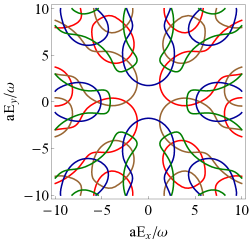
Figure 8: Merging lines as a function of the external ac electric field parameters $E_{x}$ and $E_{y}$ for the condition $\varphi=0$. The different colors label the four inequivalent $\text{M}_{j}$ points for the merging.

In addition, in this plot it is clearly seen the imprint of the lattice symmetry (hexagonal pattern) around the $\text{SM}_{0}$ phase (the one at $E_{x}=E_{y}=0$ which is connected to undriven graphene). This can be expected from the fact that linearly polarized fields do not modify the phase adquired by the electron during the hopping ($\Psi_{i}=0$ for all $i$). Thus, the effective lattice with renormalized hoppings must conserve the hexagonal symmetry. This effect can be understood as well in terms of the hoppings: Tuning the electric field orientation, we favor one of the three different hoppings. It leads to three different merging lines (blue, red and brown) and the six-fold symmetry occurs because of the positive/negative value of the field amplitude.

References

- (1) M. Hasan and C. Kane, Rev. Mod. Phys. 82, 3045 (2010).
- (2) X.-L. Qi and S.-C. Zhang, Rev. Mod. Phys. 83, 1057 (2011).
- (3) C. L. Kane and E. J. Mele, Phys. Rev. Lett. 95, 146802 (2005).
- (4) B. A. Bernevig, T. A. Hughes, and S.-C. Zhang, Science 314, 1757 (2006).
- (5) Markus Knig, Steffen Wiedmann, Christoph Brne, Andreas Roth, Hartmut Buhmann, Laurens W. Molenkamp, Xiao-Liang Qi, and Shou-Cheng Zhang et al., Science 318, 766-770 (2007).
- (6) A. H. C. Neto, F. Guinea, N. M. R. Peres, K. S. Novoselov, and A. K. Geim, Rev. Mod. Phys. 81, 109 (2009).
- (7) J.-I. Inoue and A. Tanaka, Phys. Rev. Lett. 105, 017401 (2010).
- (8) N. H. Lindner, G. Refael, and V. Galitski, Nat. Phys 7, 490 (2011).
- (9) Z. Gu, H. A. Fertig, D. P. Arovas, and A. Auerbach, Phys. Rev. Lett. 107, 216601 (2011).
- (10) T. Kitagawa, T. Oka, A. Brataas, L. Fu, and E. Demler, Phys. Rev. B 84, 235108 (2011).
- (11) A. Gómez-León and G. Platero, Phys. Rev. Lett. 110, 200403 (2013).
- (12) J. Cayssol, B. Dora, F. Simon and R. Moessner, Phys. Status Solidi RRL 7, 101 (2013).
- (13) M. C. Rechtsman et al., Nature 496, 196 (2013).
- (14) P. Dietl, F. Pichon, and G. Montambaux, Phys. Rev. Lett. 100, 236405 (2008).
- (15) B. Wunsch, F. Guinea, and F. Sols, New J. Phys. 10, 103027 (2008).
- (16) V. M. Pereira, A. H. Castro Neto, and N. M. R. Peres, Phys. Rev. B 80, 045401 (2009).
- (17) J. Zak, Phys. Rev. Lett. 62, 2747 (1988).
- (18) S. Ryu and Y. Hatsugai, Phys. Rev. Lett. 89, 077002 (2002).
- (19) P. Delplace, D. Ullmo, and G. Montambaux, Phys. Rev. B 84, 195452 (2011).
- (20) L. Tarruell, D. Greif, T. Uehlinger, G. Jotzu, and T. Esslinger, Nature 483, 302 (2012).
- (21) L.-K. Lim, J.-N. Fuchs, and G. Montambaux, Phys. Rev. Lett. 108, 175303 (2012).
- (22) M. C. Rechtsman, Y. Plotnik, J. M. Zeuner, and M. S. A. Szameit, arXiv:1211.5683 (2012).
- (23) M. Bellec, U. Kuhl, G. Montambaux, and F. Mortessagne, Phys. Rev. Lett. 110, 033902 (2013).
- (24) G. Montambaux, F. Pichon, J.-N. Fuchs, and M. O. Goerbig, Phys. Rev. B 80, 153412 (2009).
- (25) S. Koghee, L.-K. Lim, M. O. Goerbig, and C. M. Smith, Phys. Rev. A 85, 023637 (2012).
- (26) M. Busl, G. Platero, and A.-P. Jauho, Phys. Rev. B 85, 155449 (2012).
- (27) G. Platero and R. Aguado, Physics Reports 395, 1 (2004).
- (28) H. Sambe, Phys. Rev. A 7, 2203 (1973).
- (29) Á. Gómez-León, P. Delplace, and G. Platero, arXiv: 1309.5402 (2013).
- (30) G. Montambaux, F. Pichon, J.-N. Fuchs, and M.-O. Goerbig, Eur. Phys. J. B. 72, 509 (2009).
- (31) A. P. Schnyder, S. Ryu, A. Furusaki, and A. W. W. Ludwig, Phys. Rev. B 78, 195125 (2009).
- (32) A. Kundu and B. Seradjeh, Phys. Rev. Lett. 111, 136402 (2013).
- (33) E. J. G. Santos and E. Kaxiras, Nano Letters 13, 898 (2013).
- (34) J. Karch et al., Phys. Rev. Lett. 107, 276601 (2011).
- (35) S. Tani, F. M. C. Blanchard, and K. Tanaka, Phys. Rev. Lett. 109, 166603 (2012).
- (36) M. Polini, F. Guinea, M. Lewenstein, H. C. Manoharan, and V. Pellegrini, Nature Nanotechnology 8, 625–33 (2013).