Minimal predictive see-saw model with normal neutrino mass hierarchy

Abstract

We consider the type I see-saw model with two right-handed neutrinos and a normal neutrino mass hierarchy and impose a zero coupling between the right-handed neutrino mainly responsible for the atmospheric neutrino mass and the electron neutrino. We derive a master formula which relates see-saw input parameters in a one to one correspondence with physical neutrino observables. Using the master formula we search for simple ratios of couplings consistent with current data on neutrino mass and lepton mixing. We discover a minimal predictive example in which the right-handed neutrino mainly responsible for the atmospheric neutrino mass has couplings to $(\nu_{e},\nu_{\mu},\nu_{\tau})$ proportional to $(0,1,1)$ and the right-handed neutrino mainly responsible for the solar neutrino mass has couplings to $(\nu_{e},\nu_{\mu},\nu_{\tau})$ proportional to $(1,1,3)$ or $(1,3,1)$, with a relative phase $\eta=\mp\pi/3$, providing the link between leptogenesis and CP violation in neutrino oscillation experiments. We show how these patterns of couplings could arise from an $A_{4}$ family symmetry model of leptons which predicts all the PMNS parameters in terms of the neutrino mass ratio $m_{2}/m_{3}$, corresponding to Tri-bimaximal-Cabibbo mixing, accurate to one degree, with the prediction $\delta\approx\pm\pi/2$.

1 Introduction

The type I see-saw mechanism [1] provides a beautiful understanding of the smallness of neutrino masses as being due to the heavy right-handed Majorana neutrino masses. Furthermore it strongly suggests that light neutrinos are also Majorana. However, despite its attractive features, the see-saw mechanism provides no understanding of the observed bi-large lepton mixing. It also provides no insight into either the ordering (i.e. normal or inverted) or the mass scale of the neutrinos (i.e. the mass of the lightest neutrino). Moreover the see-saw mechanism is difficult to test experimentally, unless the right-handed neutrino masses are at the TeV scale [2], and typically contains more parameters than physical observables [3]. The larger number of see-saw parameters means that the neutrino Yukawa couplings cannot ever be determined from physical neutrino observables. Finally, apparently “unnatural” cancellations can take place when constructing the effective neutrino mass matrix from the see-saw parameters.

One attractive idea which avoids the last problem of “unnatural” cancellations in the see-saw mechanism is that the right-handed neutrinos contribute sequentially to the light effective neutrino mass matrix with hierarchical strength, leading to a normal mass hierarchy of physical neutrino masses $m_{3}\gg m_{2}\gg m_{1}$. This is consistent with recent Planck results which provide no evidence of quasi-degeneracy and lead to a bound [4],

$$\sum_{i}m_{i}<0.23{\rm eV}\ (95\%;Planck+WP+highL+BAO).$$ (1)

The idea of such a sequential dominance (SD) [5] of right-handed neutrinos is that one right-handed neutrino of mass $M_{\rm atm}$ dominantly contributes to the see-saw mechanism and is mainly responsible for the atmospheric neutrino mass $m_{3}$, while a second sub-dominant right-handed neutrino of mass $M_{\rm sol}$ is mainly responsible for the solar neutrino mass $m_{2}$, with a third almost decoupled right-handed neutrino of mass $M_{\rm dec}$ being mainly responsible for the lightest neutrino mass $m_{1}$. Moreover, in the limit that the lightest neutrino mass $m_{1}\rightarrow 0$, the almost decoupled right-handed neutrino becomes irrelevant and the see-saw mechanism reduces to the two right-handed neutrino case with a normal neutrino mass hierarchy, which reduces the number of see-saw parameters as we now discuss.

The type I see-saw mechanism with effectively two right-handed neutrinos [6] has fewer parameters and predicts one massless neutrino, leading to simplified formulas for neutrinoless double beta decay and the sum of neutrino masses relevant for cosmology. Texture zeros can further reduce the number of see-saw parameters [7, 8, 9, 10, 11]. With one texture zero [7, 10], the $3\times 2$ neutrino Yukawa matrix contains 7 real parameters, after charged lepton phase rotations, which is exactly the same number of parameters as non-zero physical neutrino observables, comprising 2 real positive masses $m_{2},m_{3}$, the 3 mixing angles $\theta_{23},\theta_{13},\theta_{12}$, the oscillation phase $\delta$ and the single Majorana phase $\beta$.

In the case of the two right-handed neutrino model with a normal hierarchy, if the “dominant” right-handed neutrino has zero coupling to the lepton doublet containing the electron, this was shown over a decade ago to bound the reactor angle $\theta_{13}\stackrel{{\scriptstyle<}}{{{}_{\sim}}}m_{2}/m_{3}$ [7, 10]. We shall refer to this zero coupling as a “dominant texture zero”. For example, such a “dominant texture zero” could appear in the (1,1) entry of the neutrino Yukawa matrix, similar to the quark and charged lepton Yukawa matrices, where a (1,1) texture zero it is a key ingredient of the Gatto-Sartori-Tonin (GST) [12] and Georgi-Jarlskog (GJ) relations [13]. Recently, Daya Bay [14] and RENO [15] have measured $\theta_{13}\approx 0.15$ near the upper limit of the bound $\theta_{13}\stackrel{{\scriptstyle<}}{{{}_{\sim}}}m_{2}/m_{3}$ [7, 10]. The fact that this bound is saturated could be indicative of a particular underlying pattern of Yukawa couplings, and this provides part of the motivation for revisiting the minimal see-saw model. In particular we shall derive a new “master formula” which relates physical observables to Yukawa couplings, providing the necessary tools for such questions to be addressed.

The measurement of a non-zero reactor angle excludes tri-bimaximal (TB) mixing [16]. It is nevertheless convenient to express the $s$olar, $a$tmospheric and $r$eactor angles in terms of (small) deviation parameters ($s$, $a$ and $r$) from TB mixing [17] (for a related parametrisation see [18]):

$$\sin\theta_{12}=\frac{1}{\sqrt{3}}(1+s),\ \ \ \ \sin\theta_{23}=\frac{1}{\sqrt{2}}(1+a),\ \ \ \ \sin\theta_{13}=\frac{r}{\sqrt{2}}.$$ (2)

For example, following the Daya Bay and RENO results, it was pointed out that the lepton mixing angles are consistent with the so called Tri-bimaximal-Cabibbo (TBC) ansatz [19] where

$$s=0,\ \ \ \ a=0,\ \ \ \ r=\lambda,$$ (3)

corresponding to

$$\sin\theta_{12}=\frac{1}{\sqrt{3}},\ \ \ \ \sin\theta_{23}=\frac{1}{\sqrt{2}},\ \ \ \ \sin\theta_{13}=\frac{\lambda}{\sqrt{2}},$$ (4)

with $\lambda=0.225$ being the Wolfenstein parameter, yielding the TBC angles,

$$\theta_{12}=35.26^{\circ},\ \ \ \ \theta_{23}=45^{\circ},\ \ \ \ \theta_{13}=9.15^{\circ}.$$ (5)

The TBC lepton mixing matrix is given to second order by [19],

$$V_{\mathrm{TBC}}\approx\left(\begin{array}[]{ccc}\sqrt{\frac{2}{3}}(1-\frac{1}{4}\lambda^{2})&\frac{1}{\sqrt{3}}(1-\frac{1}{4}\lambda^{2})&\frac{1}{\sqrt{2}}\lambda e^{-i\delta}\\ -\frac{1}{\sqrt{6}}(1+\lambda e^{i\delta})&\frac{1}{\sqrt{3}}(1-\frac{1}{2}\lambda e^{i\delta})&\frac{1}{\sqrt{2}}(1-\frac{1}{4}\lambda^{2})\\ \frac{1}{\sqrt{6}}(1-\lambda e^{i\delta})&-\frac{1}{\sqrt{3}}(1+\frac{1}{2}\lambda e^{i\delta})&\frac{1}{\sqrt{2}}(1-\frac{1}{4}\lambda^{2})\end{array}\right)+\mathcal{O}(\lambda^{3}).$$ (6)

TBC mixing thus assumes maximal atmospheric mixing and trimaximal solar mixing. For the normal neutrino mass hierarchy, some of the global fits, reviewed in [20], prefer an alternative ansatz which we refer to as TBC2, corresponding to,

$$s=-\lambda^{2},\ \ \ \ a=-\lambda/2,\ \ \ \ r=\lambda.$$ (7)

This TBC2 ansatz has the feature that the atmospheric mixing angle is in the first octant and the solar mixing angle is somewhat less than its tri-maximal value as preferred by some of the latest global fits at the one sigma level, while TBC mixing generally remains valid at the three sigma level or better for all the global fits [20]. We emphasise that the issue of whether the atmospheric angle is maximal or not remains unresolved, with SuperKamiokande having a mild preference for a non-maximal atmospheric angle [21] while T2K prefers a maximal atmospheric angle, although both preferences are less than one sigma and hence not statistically significant. This situation is expected to be clarified in the near future. Returning to our analysis, the ansatze we have used will serve as an approximate guide in searching for particular patterns of Yukawa couplings. Once a particular pattern is identified, it then takes a life of its own, independently of the TBC or TBC2 ansatz, and leads to predictions for lepton mixing independently of either of these two ansatze which were used to discover the pattern in the first place.

The present paper divides into two parts. In the first part we shall perform a model independent analysis of the two right-handed neutrino model with a normal neutrino mass hierarchy and a single “dominant texture zero” in the electron component of the Yukawa matrix [7, 10]. This model provides an attractive and rather minimal extension of the Standard Model consistent with all current neutrino data, with a one to one correspondence between the Yukawa couplings and the physical observables. We shall derive a master formula comprising exact analytic results which express the Yukawa couplings in terms of general values of the physical masses and mixings. These results in principle do not rely on the SD assumption and are valid even for large values of reactor angle. However we show that, in practice, the observed reactor angle $\theta_{13}\stackrel{{\scriptstyle<}}{{{}_{\sim}}}m_{2}/m_{3}$ implies and is implied by SD, where the “texture zero” in the electron component becomes the “dominant texture zero”. We also confirm that a second texture zero is not possible, at least without invoking charged lepton corrections which we do not consider in this paper. In fact the two right-handed neutrino model with two texture zeros [8, 9, 11] was recently shown to be not viable for the normal hierarchy case [23, 24], which provides a further reason why we mainly focus on the one texture zero case [7, 10, 11] here.

The second part of the paper is concerned with applying the results obtained in the first part to model building. An important step in this direction is to use the master formula to derive exact analytic results for the ratios of Yukawa couplings in terms of physical neutrino observables, and to use these results, together with the current best fit values of neutrino masses and mixing angles, to search for simple patterns of Yukawa couplings. We find that the atmospheric neutrino mass can have couplings to $(\nu_{e},\nu_{\mu},\nu_{\tau})$ proportional to, for example, $(0,1,1)$ or $(0,1,2)$, which are strongly dependent on the value of the CP violating oscillation phase $\delta$. The right-handed neutrino mainly responsible for the solar neutrino mass can have couplings to $(\nu_{e},\nu_{\mu},\nu_{\tau})$ proportional to $(1,4,2)$ or $(1,1,3)$ or $(1,3,1)$, which are strongly dependent on the value of both the oscillation phase and the Majorana phase and differ from the traditional constrained sequential dominance (CSD) values [25]. In particular we focus on CSD3 defined to be based on the atmospheric couplings $(0,1,1)$ and the solar couplings being either $(1,1,3)$ or $(1,3,1)$, with a relative phase difference $\eta=\mp\pi/3$. We show how these patterns of couplings could arise from an $A_{4}$ family symmetry model of leptons which predicts all the PMNS parameters in terms of the neutrino mass ratio $m_{2}/m_{3}$, corresponding to approximate Tri-bimaximal-Cabibbo mixing to an accuracy of one degree with $\delta\approx\pm\pi/2$. The model provides a link between leptogenesis and CP violation in neutrino oscillation experiments.

We remark that, although the two right-handed neutrino model with one texture zero case has been discussed before [7, 10, 11], such studies were performed about a decade ago when the mixing angles were not known so precisely, so it is timely to revisit them, in the light of the first measurement of the reactor angle by Daya Bay and RENO which approximately saturates the “dominant texture zero” bound $\theta_{13}\stackrel{{\scriptstyle<}}{{{}_{\sim}}}m_{2}/m_{3}$ [7, 10]. Moreover, as indicated above, we present new and exact analytic results which directly relate Yukawa couplings to physical neutrino observables. Previously in [7, 10] only approximate relations were given, while in [11] exact relations between Yukawa couplings and physical neutrino observables were only given parametrically via the complex angle $z$ arising from an orthogonal parametrisation. Here we give a simple derivation of exact analytic relations between Yukawa couplings and physical neutrino observables via a master formula which does not rely on any parameterisation. We also emphasise a further important difference between the present paper and the earlier ones is that we know now that the bound $\theta_{13}\stackrel{{\scriptstyle<}}{{{}_{\sim}}}m_{2}/m_{3}$ is approximately saturated, and in this paper we seek a simple answer to this question in terms of ratios of Yukawa couplings with simple phase relations. The fact that we find a simple answer, namely CSD3, is very gratifying, since it opens up new possibilities for model building as well as linking leptogenesis to the PMNS phases. We go on to construct an explicit $A_{4}$ model of leptons for one of the examples that completely determines the PMNS mixing matrix including all the phases.

The layout of the remainder of this paper is as follows. In the first part of the paper we perform a model independent analysis. In section 2 we briefly show how the two right-handed neutrino model emerges as the limiting case of a three right-handed neutrino model with sequential dominance. In section 3 we discuss the two right-handed neutrino with a normal neutrino mass hierarchy and a texture zero in the electron component of either one of the two right-handed neutrinos, and derive a master formula relating see-saw parameters to physical parameters for this case. Using the master formula we show that SD emerges as a consequence of bi-large mixing and the observed reactor angle, with the texture zero being associated with the dominant right-handed neutrino. In section 4, using the master formula, we calculate ratios of Yukawa couplings and see-saw phases, as functions of the PMNS phases, for particular mixing patterns such as TBC and TBC2 which are consistent with present data.

In the second part of the paper we discuss the implications of the results for model building. After a brief review in section 5 of the status of indirect models, in section 6 we scrutinise the results obtained in the previous section, looking for simple possibilities which could form the basis of new indirect models. We discuss three such examples in some detail, checking their viability using exact numerical results for PMNS parameters and leading order approximate analytic results in section 7. We also discuss the link between leptogenesis and PMNS phases in section 8. In section 9 we then focus on CSD3 based on the alignment $(0,1,1)$ for the atmospheric column and $(1,1,3)$ or $(1,3,1)$ for the solar column with a relative phase difference $\eta=\mp\pi/3$ and show how these follow from $A_{4}$ family symmetry model of leptons based on F-term vacuum alignment and spontaneous CP violation. The model predicts all the PMNS mixing parameters in terms of the neutrino mass ratio, corresponding to approximate Tri-bimaximal-Cabibbo mixing to an accuracy of one degree with $\delta\approx\pm\pi/2$. Section 10 concludes the paper.

2 Two Right-Handed Neutrino Model as a Limiting Case of Sequential Dominance

The starting point for our analysis is the see-saw mechanism in the flavour basis where the charged lepton mass matrix $M_{E}$ is diagonal with real positive eigenvalues $m_{e},m_{\mu},m_{\tau}$ and the three right-handed neutrino Majorana mass matrix $M_{R}$ is also diagonal, with real positive eigenvalues, $M_{\rm atm},M_{\rm sol},M_{\rm dec}$,

$$M_{E}=\left(\begin{array}[]{ccc}m_{e}&0&0\\ 0&m_{\mu}&0\\ 0&0&m_{\tau}\end{array}\right),\ M_{R}=\left(\begin{array}[]{ccc}M_{\rm atm}&0&0\\ 0&M_{\rm sol}&0\\ 0&0&[M_{\rm dec}]\end{array}\right).$$ (8)

We write the neutrino Dirac mass matrix as

$$m^{D}=\left(\begin{array}[]{ccc}m^{D}_{e,\rm atm}&m^{D}_{e,\rm sol}&[m^{D}_{e,\rm dec}]\\ m^{D}_{\mu,\rm atm}&m^{D}_{\mu,\rm sol}&[m^{D}_{\mu,\rm dec}]\\ m^{D}_{\tau,\rm atm}&m^{D}_{\tau,\rm sol}&[m^{D}_{\tau,\rm dec}]\end{array}\right)\equiv\left(\begin{array}[]{ccc}m^{D}_{\rm atm}&m^{D}_{\rm sol}&[m^{D}_{\rm dec}]\end{array}\right),$$ (9)

in the convention where the effective Lagrangian after electroweak symmetry breaking, with the Higgs vacuum expectation value (vev) inserted, is given by

$${\cal L}=-\overline{E_{L}}M_{E}E_{R}-\overline{\nu_{L}}m^{D}N_{R}-\frac{1}{2}\overline{N_{R}^{c}}M_{R}N_{R}+{H.c.}\;,$$ (10)

where $\nu_{L}=(\nu_{e},\nu_{\mu},\nu_{\tau})$ are the three left-handed neutrino fields which appear together with $E_{L}=(e_{L},\mu_{L},\tau_{L})$ in the lepton doublets $L=(L_{e},L_{\mu},L_{\tau})$ and $N_{R}=(N_{\rm atm},N_{\rm sol},N_{\rm dec})$ are the three right-handed neutrinos and we have defined the three Dirac column vectors as $m^{D}_{\rm atm}$, $m^{D}_{\rm sol}$, $m^{D}_{\rm dec}$.

The term for the light neutrino masses in the effective Lagrangian (after electroweak symmetry breaking), resulting from integrating out the massive right handed neutrinos (i.e. the see-saw mechanism with the light effective neutrino Majorana mass matrix $m^{\nu}=m^{D}M_{R}^{-1}{m^{D}}^{T}$) is

$$\mathcal{L}^{\nu}_{eff}=\frac{(\overline{\nu_{L}}m^{D}_{\rm atm})({m^{D}_{\rm atm}}^{T}\nu_{L}^{c})}{M_{\rm atm}}+\frac{(\overline{\nu_{L}}m^{D}_{\rm sol})({m^{D}_{\rm sol}}^{T}\nu_{L}^{c})}{M_{\rm sol}}\ \left[\ +\frac{(\overline{\nu_{L}}m^{D}_{\rm dec})({m^{D}_{\rm dec}}^{T}\nu_{L}^{c})}{M_{\rm dec}}\ \right].$$ (11)

Sequential dominance (SD) then corresponds to the third term being negligible, the second term subdominant and the first term dominant:

$$\frac{m^{D}_{\rm atm}{m^{D}_{\rm atm}}^{T}}{M_{\rm atm}}\gg\frac{m^{D}_{\rm sol}{m^{D}_{\rm sol}}^{T}}{M_{\rm sol}}\ \left[\ \gg\frac{m^{D}_{\rm dec}{m^{D}_{\rm dec}}^{T}}{M_{\rm dec}}\ \right]\,,$$ (12)

which immediately predicts a normal neutrino mass hierarchy,

$$m_{3}\gg m_{2}\ \left[\ \gg m_{1}\ \right],$$ (13)

which is the main prediction of SD.

We have labelled the dominant right-handed neutrino and Yukawa couplings mainly responsible for the atmospheric neutrino mass $m_{3}$ as “${\rm atm}$”, the subdominant ones mainly responsible for the solar neutrino mass $m_{2}$ as “${\rm sol}$”, and the almost decoupled (sub-sub-dominant) ones mainly responsible for $m_{1}$ as “${\rm dec}$”. Note that the mass ordering of right-handed neutrinos is not yet specified. We shall order the right-handed neutrino masses as $M_{1}<M_{2}<M_{3}$, and subsequently identify $M_{\rm atm},M_{\rm sol},M_{\rm dec}$ with $M_{1},M_{2},M_{3}$ in all possible ways.

It is clear that in the limit that $m_{1}\rightarrow 0$ then the sub-sub-dominant right-handed neutrino and its associated couplings labelled by “${\rm dec}$” decouple completely and the above model reduces to a two right-handed neutrino model. In that limit we simply drop the third terms [in square brackets] in Eqs.8-13 in anticipation of this.

3 The Two Right-Handed Neutrino Model with Normal Hierarchy and Dominant Texture Zero

3.1 Derivation of the Master Formula

Without assuming SD, we write the see-saw matrices in a simple notation as,

$$m^{D}=\left(\begin{array}[]{cc}0&a\\ e&b\\ f&c\end{array}\right),\ \ \ \ M_{R}=\left(\begin{array}[]{cc}Y&0\\ 0&X\end{array}\right).$$ (14)

where we have written the complex Dirac masses as $a,b,c,d,e,f$ with $d=0$ and the real positive right-handed neutrino masses as $Y,X$. We are in a basis where the charged lepton mass matrix $M_{E}$ is diagonal with real positive eigenvalues ordered as $m_{e},m_{\mu},m_{\tau}$. Later on we shall show that the observed reactor angle $\theta_{13}\stackrel{{\scriptstyle<}}{{{}_{\sim}}}m_{2}/m_{3}$ implies and is implied by SD, where the “texture zero” in the electron component becomes the “dominant texture zero”, i.e. we will later identify $d=m^{D}_{e,\rm atm}=0$ and $Y=M_{\rm atm}$ in the notation of the previous section. However, to begin with, we do not presume this identification. We also allow the real positive right-handed neutrino masses $Y$ and $X$ to have either mass ordering, i.e. namely $Y=M_{1}$ or $Y=M_{2}$ where $M_{1}<M_{2}$. Hence the texture zero in Eq.14 covers both cases with a texture zero in the electron component,

$$m^{D}=\left(\begin{array}[]{cc}0&\times\\ \times&\times\\ \times&\times\end{array}\right),\ \ \ \ \left(\begin{array}[]{cc}\times&0\\ \times&\times\\ \times&\times\end{array}\right).$$ (15)

We now derive a master formula in which the see-saw parameters in Eq.14 may be related to the low energy physical observables such as neutrino masses, mixing angles and physical phases. Integrating out the right-handed neutrinos the see-saw formula gives the approximate light effective Majorana neutrino mass matrix,

$$m^{\nu}=-m^{D}M_{R}^{-1}{m^{D}}^{T}\ .$$ (16)

in the convention where the effective Lagrangian is given by

$${\cal L}=-\overline{E_{L}}M_{E}E_{R}-\frac{1}{2}\overline{\nu_{L}}m^{\nu}\nu_{L}^{c}+{H.c.}\;.$$ (17)

Performing the transformation from the flavour basis to the real positive mass basis by,

$$V_{E_{L}}\,M_{E}\,V^{\dagger}_{E_{R}}=\mbox{diag}(m_{e},m_{\mu},m_{\tau}),\quad~{}V_{\nu_{L}}\,m^{\nu}\,V^{T}_{\nu_{L}}=\mbox{diag}(m_{1},m_{2},m_{3}),$$ (18)

the PMNS matrix is given by

$$U=V_{E_{L}}V^{\dagger}_{\nu_{L}}\,.$$ (19)

Since, as before, we are in the basis where the charged lepton mass matrix $M_{E}$ is already diagonal, then in general $V_{E_{L}}$ can only be a diagonal matrix,

$$V_{E_{L}}=P_{E}=\left(\begin{array}[]{ccc}e^{i\phi_{e}}&0&0\\ 0&e^{i\phi_{\mu}}&0\\ 0&0&e^{i\phi_{\tau}}\end{array}\right),$$ (20)

consisting of arbitrary phases, where an identical phase rotation on the right-handed charged leptons $V_{E_{R}}=P_{E}$ leaves the diagonal charged lepton masses in $M_{E}$ unchanged. In practice the phases in $P_{E}$ are chosen to absorb three phases from the unitary matrix $V^{\dagger}_{\nu_{L}}$ and to put $U$ in a standard convention,

$$U=VP$$ (21)

where, analogous to the CKM matrix,

$$V=\left(\begin{array}[]{ccc}c_{12}c_{13}&s_{12}c_{13}&s_{13}e^{-i\delta}\\ -s_{12}c_{23}-c_{12}s_{13}s_{23}e^{i\delta}&\hphantom{+}c_{12}c_{23}-s_{12}s_{13}s_{23}e^{i\delta}&c_{13}s_{23}\\ \hphantom{+}s_{12}s_{23}-c_{12}s_{13}c_{23}e^{i\delta}&-c_{12}s_{23}-s_{12}s_{13}c_{23}e^{i\delta}&c_{13}c_{23}\end{array}\right),$$ (25)

and the Majorana phase matrix factor is,

$$P=\left(\begin{array}[]{ccc}e^{i\frac{\beta_{1}}{2}}&0&0\\ 0&e^{i\frac{\beta_{2}}{2}}&0\\ 0&0&1\\ \end{array}\right).$$ (26)

From Eqs.18,19,20, we find,

$$U^{\dagger}P_{E}m^{\nu}P_{E}U^{*}=\mbox{diag}(m_{1},m_{2},m_{3}).$$ (27)

Then using Eq.21 we find

$$V^{\dagger}P_{E}m^{\nu}P_{E}V^{*}=P\mbox{diag}(m_{1},m_{2},m_{3})P=\mbox{diag}(0,e^{i\beta}m_{2},m_{3}),$$ (28)

where we have dropped $m_{1}=0$ (since we are considering the two right-handed neutrino model with a normal mass hierarchy) and defined $\beta\equiv\beta_{2}$. Using the see-saw formula, Eq.16, this may be written,

$$-P_{E}m^{D}M_{R}^{-1}{m^{D}}^{T}P_{E}=V\mbox{diag}(0,e^{i\beta}m_{2},m_{3})V^{T},$$ (29)

or,

$$m^{D^{\prime}}M_{R}^{-1}{m^{D^{\prime}}}^{T}=V\mbox{diag}(0,e^{i\beta}m_{2},m_{3})V^{T},$$ (30)

where,

$$m^{D^{\prime}}=iP_{E}m^{D}=i\left(\begin{array}[]{ccc}e^{i\phi_{e}}&0&0\\ 0&e^{i\phi_{\mu}}&0\\ 0&0&e^{i\phi_{\tau}}\end{array}\right)\left(\begin{array}[]{cc}0&a\\ e&b\\ f&c\end{array}\right).$$ (31)

Finally, expanding Eq.30 using Eqs. 14 and 31, we arrive at our “master formula”,

$$\left(\begin{array}[]{ccc}\tilde{a}^{2}&\tilde{a}\tilde{b}&\tilde{a}\tilde{c}\\ \tilde{a}\tilde{b}&\tilde{e}^{2}+\tilde{b}^{2}&\tilde{e}\tilde{f}+\tilde{b}\tilde{c}\\ \tilde{a}\tilde{c}&\tilde{e}\tilde{f}+\tilde{b}\tilde{c}&\tilde{f}^{2}+\tilde{c}^{2}\end{array}\right)_{\alpha\beta}=e^{i\beta}m_{2}V_{\alpha 2}V_{\beta 2}+m_{3}V_{\alpha 3}V_{\beta 3},$$ (32)

where we have defined

$$\tilde{a}\equiv\frac{ie^{i\phi_{e}}a}{\sqrt{X}},\ \ \tilde{b}\equiv\frac{ie^{i\phi_{\mu}}b}{\sqrt{X}},\ \ \tilde{c}\equiv\frac{ie^{i\phi_{\tau}}c}{\sqrt{X}},\ \ \tilde{e}\equiv\frac{ie^{i\phi_{\mu}}e}{\sqrt{Y}},\ \ \tilde{f}\equiv\frac{ie^{i\phi_{\tau}}f}{\sqrt{Y}}.$$ (33)

The “master formula” in Eq.32 is a very useful equation, since it relates the re-phased Dirac mass matrix parameters $a,b,c,e,f$, scaled by the positive square roots of the right-handed neutrino masses $X,Y$, which are the inputs of the see-saw mechanism (see Eq. 14), to physical low energy observables. The combinations of see-saw input parameters appear on the LHS of Eq.32 while the physical neutrino masses, mixing angles and phases appear on the RHS of Eq.32.

In terms of parameter counting, we see that the RHS of the “master formula” Eq.32, with $V$ in Eq.25, involves 7 non-zero physical parameters, comprising 2 real positive masses $m_{2},m_{3}$, the 3 mixing angles $\theta_{23},\theta_{13},\theta_{12}$, the oscillation phase $\delta$ and the single Majorana phase $\beta$, which determine exactly the 5 complex parameters $\tilde{a},\tilde{b},\tilde{c},\tilde{e},\tilde{f}$ on the LHS which therefore involve only two independent physical phases. We shall refer to $\tilde{a},\tilde{b},\tilde{c},\tilde{e},\tilde{f}$ as the “physical see-saw parameter combinations”. Note that the 5 input complex Dirac masses $a,b,c,e,f$ also only depend on two physical phase differences which are left invariant under charged lepton re-phasing as discussed further later.

3.2 Sequential Dominance and the Dominant Texture Zero

So far we have considered the two right-handed neutrino model with a single texture zero in the electron component, assuming a normal neutrino mass hierarchy, and have derived a “master formula” in Eq.32, relating see-saw parameters to physical observables. As a first application of this formula, we show that SD is a consequence of the assumed texture zero $d=0$ which turns out to be the “dominant texture zero”.

Writing out the “master formula” Eq.32 explicitly for all $(\alpha,\beta)$ gives,

$$\tilde{a}^{2} = e^{i\beta}m_{2}V_{12}^{2}+m_{3}V_{13}^{2},$$ (34)

$$\tilde{a}\tilde{b} = e^{i\beta}m_{2}V_{12}V_{22}+m_{3}V_{13}V_{23},$$ (35)

$$\tilde{a}\tilde{c} = e^{i\beta}m_{2}V_{12}V_{32}+m_{3}V_{13}V_{33},$$ (36)

$$\tilde{e}\tilde{f}+\tilde{b}\tilde{c} = e^{i\beta}m_{2}V_{22}V_{32}+m_{3}V_{23}V_{33},$$ (37)

$$\tilde{e}^{2}+\tilde{b}^{2} = e^{i\beta}m_{2}V_{22}^{2}+m_{3}V_{23}^{2},$$ (38)

$$\tilde{f}^{2}+\tilde{c}^{2} = e^{i\beta}m_{2}V_{32}^{2}+m_{3}V_{33}^{2}.$$ (39)

We can solve for the individual parameters in terms of the above combinations,

$$\tilde{b}^{2} = \frac{(\tilde{a}\tilde{b})^{2}}{\tilde{a}^{2}},$$ (40)

$$\tilde{c}^{2} = \frac{(\tilde{a}\tilde{c})^{2}}{\tilde{a}^{2}},$$ (41)

$$\tilde{e}^{2} = (\tilde{e}^{2}+\tilde{b}^{2})-\tilde{b}^{2},$$ (42)

$$\tilde{f}^{2} = (\tilde{f}^{2}+\tilde{c}^{2})-\tilde{c}^{2}.$$ (43)

Using Eqs.34-39 and TBC mixing in Eq.6, we estimate, to leading order in $\lambda$,

$$\tilde{a}^{2} \sim e^{i\beta}\frac{m_{2}}{3},$$ (44)

$$\tilde{a}\tilde{b} \sim e^{i\beta}\frac{m_{2}}{3}+e^{-i\delta}\frac{\lambda m_{3}}{2},$$ (45)

$$\tilde{a}\tilde{c} \sim -e^{i\beta}\frac{m_{2}}{3}+e^{-i\delta}\frac{\lambda m_{3}}{2},$$ (46)

$$\tilde{e}^{2}+\tilde{b}^{2} \sim \frac{m_{3}}{2},$$ (47)

$$\tilde{f}^{2}+\tilde{c}^{2} \sim \frac{m_{3}}{2}.$$ (48)

Since the mass ratio may be approximated as $m_{2}/m_{3}\approx\theta_{13}\approx\lambda/\sqrt{2}$, from Eqs.44-48 we conclude that,

$$(\tilde{e}+\tilde{f})^{2}\gg(\tilde{a}+\tilde{b}+\tilde{c})^{2}$$ (49)

since the LHS is of order $m_{3}$, while the RHS is of order $m_{2}$. Using Eq.33, we see that Eq.49 just corresponds to the SD condition in Eq.12 where we identify the see-saw matrices in Eq.14 with the notation in Section 2,

$$\left(\begin{array}[]{cc}0&a\\ e&b\\ f&c\end{array}\right)\equiv\left(\begin{array}[]{cc}m^{D}_{e,\rm atm}&m^{D}_{e,\rm sol}\\ m^{D}_{\mu,\rm atm}&m^{D}_{\mu,\rm sol}\\ m^{D}_{\tau,\rm atm}&m^{D}_{\tau,\rm sol}\end{array}\right),\ \ \ \ \left(\begin{array}[]{cc}Y&0\\ 0&X\end{array}\right)\equiv\left(\begin{array}[]{cc}M_{\rm atm}&0\\ 0&M_{\rm sol}\end{array}\right),$$ (50)

from which we see that the texture zero in the electron component is in fact the “dominant texture zero”, since we identify $m^{D}_{e,\rm atm}=0$ and $Y=M_{\rm atm}$. From our present perspective, where the reactor angle is measured, we see that SD and the “dominant texture zero” implies and is implied by the data on the mixing angles which is approximated here by TBC mixing. However, historically, a decade before the measurement of $\theta_{13}$, SD was simply postulated, along with the “dominant texture zero”. This was then shown to lead to the bound on the reactor angle $\theta_{13}\stackrel{{\scriptstyle<}}{{{}_{\sim}}}m_{2}/m_{3}$ using approximate analytic formulas for the mixing angles and phases expressed in terms of input see-saw parameters [7, 10].

3.3 Excluding a second texture zero

In this subsection we use the “master formula” in Eq.32 to search for simple patterns of neutrino Dirac masses, or equivalently neutrino Yukawa couplings, which could motivate some future flavour model, for example based on a discrete family symmetry. To address such questions, it is relevant to take the ratios of the see-saw parameters in the same Dirac column, so that the right-handed neutrino masses cancel. From Eqs.34-39 and Eq.33 we find,

$$z_{1}\equiv\frac{\tilde{e}}{\tilde{f}} = \pm\frac{V_{23}V_{12}-V_{13}V_{22}}{V_{33}V_{12}-V_{13}V_{32}}$$ (51)

$$z_{2}\equiv\frac{\tilde{b}}{\tilde{a}} = \frac{e^{i\beta}m_{2}V_{12}V_{22}+m_{3}V_{13}V_{23}}{e^{i\beta}m_{2}V_{12}^{2}+m_{3}V_{13}^{2}}$$ (52)

$$z_{3}\equiv\frac{\tilde{c}}{\tilde{a}} = \frac{e^{i\beta}m_{2}V_{12}V_{32}+m_{3}V_{13}V_{33}}{e^{i\beta}m_{2}V_{12}^{2}+m_{3}V_{13}^{2}}.$$ (53)

Note that $z_{1}$ is independent of neutrino masses (and phases). It is also worth emphasising that, using Eq.33, the moduli of these ratios are equal to the moduli of the original Dirac mass matrix elements,

$$|z_{1}|=\frac{|e|}{|f|},\ \ \ \ |z_{2}|=\frac{|b|}{|a|},\ \ \ \ |z_{3}|=\frac{|c|}{|a|}.$$ (54)

For the case of TBC2 mixing in Eq.7, we find,

$$V_{11} = \sqrt{\frac{2}{3}}(1+\frac{1}{4}\lambda^{2})$$ (55)

$$V_{12} = \frac{1}{\sqrt{3}}(1-\frac{5}{4}\lambda^{2})$$ (56)

$$V_{13} = \frac{1}{\sqrt{2}}\lambda e^{-i\delta}$$ (57)

$$V_{21} = -\frac{1}{\sqrt{6}}(1+\frac{1}{2}\lambda+\lambda e^{i\delta}-\frac{5}{4}\lambda^{2}-\frac{1}{2}\lambda^{2}e^{i\delta})$$ (58)

$$V_{22} = \frac{1}{\sqrt{3}}(1+\frac{1}{2}\lambda-\frac{1}{2}\lambda e^{i\delta}+\frac{1}{4}\lambda^{2}+\frac{1}{4}\lambda^{2}e^{i\delta})$$ (59)

$$V_{23} = \frac{1}{\sqrt{2}}(1-\frac{1}{2}\lambda-\frac{1}{4}\lambda^{2})$$ (60)

$$V_{31} = \frac{1}{\sqrt{6}}(1-\frac{1}{2}\lambda-\lambda e^{i\delta}-\lambda^{2}-\frac{1}{2}\lambda^{2}e^{i\delta})$$ (61)

$$V_{32} = -\frac{1}{\sqrt{3}}(1-\frac{1}{2}\lambda+\frac{1}{2}\lambda e^{i\delta}+\frac{1}{2}\lambda^{2}-\frac{1}{4}\lambda^{2}e^{i\delta})$$ (62)

$$V_{33} = \frac{1}{\sqrt{2}}(1+\frac{1}{2}\lambda-\frac{1}{2}\lambda^{2}).$$ (63)

We shall approximate the mass ratio as:

$$\frac{m_{2}}{m_{3}}\equiv\epsilon\approx\frac{\lambda}{\sqrt{2}}+\frac{1}{3}\lambda^{2}\approx 0.176.$$ (64)

According to the global fits, which are compared in [20], the mass ratio lies in the one sigma range $m_{2}/m_{3}=0.17-0.18$.

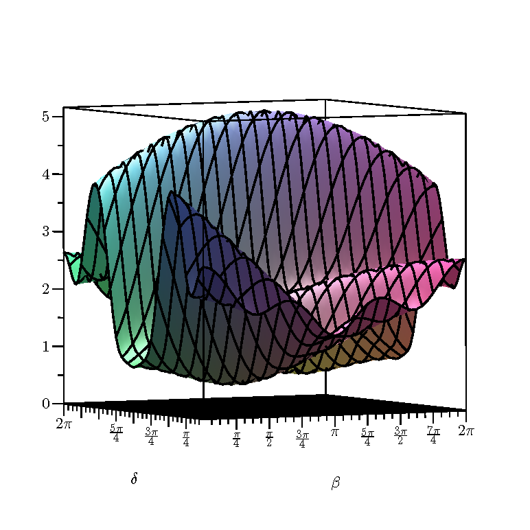
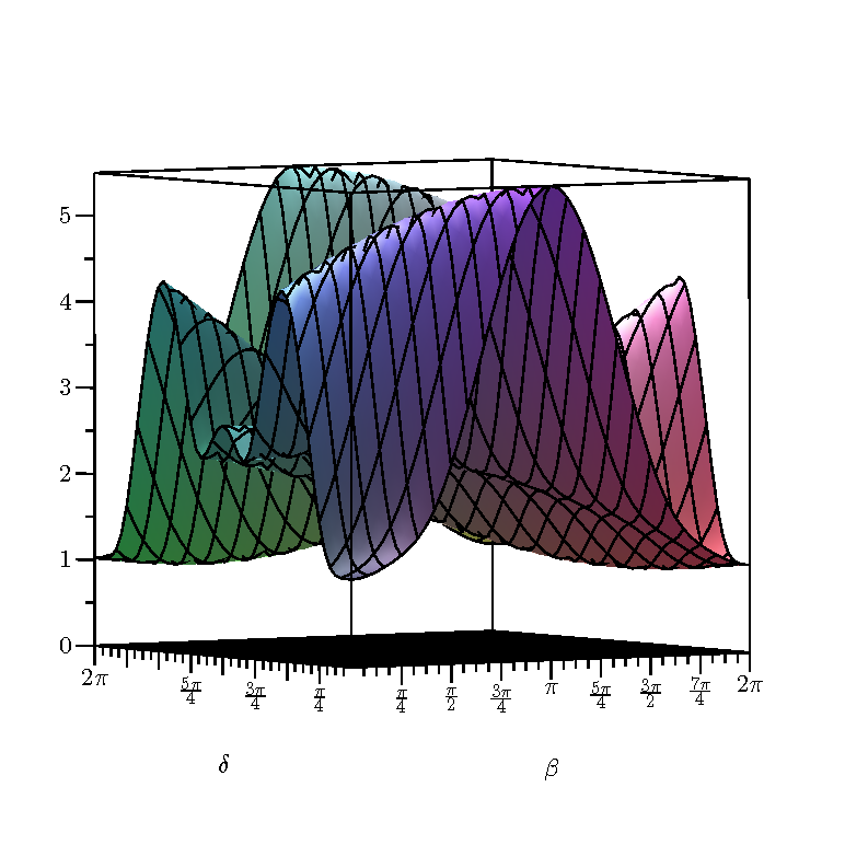
Figure 1: The left and right panels show $|z_{2}|$ and $|z_{3}|$ (respectively) as functions of the physical phases $\delta$ and $\beta$ evaluated using Eqs.52,53 and using the TBC2 ansatz in Eq.4, working to second order in $\lambda$. From these plots we see that a second texture zero corresponding to either $|z_{2}|=0$ or $|z_{3}|=0$ is not possible. Similar results are obtained for TBC mixing.

Using these approximations we perform an expansion of the ratios including terms of order $\lambda^{2}$, which we use for our numerical results. However, since the full expansion is not very instructive, we only write out the terms to order $\lambda$ below:

$$z_{1}\equiv\frac{\tilde{e}}{\tilde{f}} = \pm[1-\lambda(1+2e^{-i\delta})]+{\cal O}(\lambda^{2})$$ (65)

$$z_{2}\equiv\frac{\tilde{b}}{\tilde{a}} = 1+\frac{3}{\sqrt{2}}e^{-i(\beta+\delta)}+\frac{1}{2}\lambda(B-C)+{\cal O}(\lambda^{2})$$ (66)

$$z_{3}\equiv\frac{\tilde{c}}{\tilde{a}} = -1+\frac{3}{\sqrt{2}}e^{-i(\beta+\delta)}+\frac{1}{2}\lambda(B+C)+{\cal O}(\lambda^{2}),$$ (67)

where we have introduced the complex notation,

$$B = 1-e^{i\delta}-2e^{-i(\beta+\delta)}-9e^{-i(2\beta+3\delta)}$$ (68)

$$C = 3\sqrt{2}e^{-i(\beta+2\delta)}+\frac{3}{\sqrt{2}}e^{-i(\beta+\delta)}.$$ (69)

We can use these results to investigate the viability of a second texture zero. Apparently a second texture zero with $|a|=0$ is inconsistent with Eqs.66,67. Also either $|e|=0$ or $|f|=0$ is inconsistent with Eq.65. A second texture zero with either $|b|=0$ or $|c|=0$ would correspond to either $|z_{2}|=0$ or $|z_{3}|=0$. This looks unlikely to be possible from the leading order results, but requires numerical investigation to be sure. We find that, for both TBC mixing and the more accurate TBC2 parameterisation given by Eqs.55-63, to second order in $\lambda$, either $|z_{2}|=0$ or $|z_{3}|=0$ are not possible. This is illustrated for the second case of TBC2 mixing in Fig.1. In summary, we conclude that all the following two texture zero cases are not viable,

$$m^{D} = \left(\begin{array}[]{cc}0&\times\\ 0&\times\\ \times&\times\end{array}\right),\ \ \left(\begin{array}[]{cc}0&\times\\ \times&\times\\ 0&\times\end{array}\right),\ \ \left(\begin{array}[]{cc}0&0\\ \times&\times\\ \times&\times\end{array}\right),\ \ \left(\begin{array}[]{cc}0&\times\\ \times&0\\ \times&\times\end{array}\right),\ \ \left(\begin{array}[]{cc}0&\times\\ \times&\times\\ \times&0\end{array}\right),$$ (98)

$$\left(\begin{array}[]{cc}\times&0\\ \times&0\\ \times&\times\end{array}\right),\ \ \left(\begin{array}[]{cc}\times&0\\ \times&\times\\ \times&0\end{array}\right),\ \ \left(\begin{array}[]{cc}\times&0\\ 0&\times\\ \times&\times\end{array}\right),\ \ \left(\begin{array}[]{cc}\times&0\\ \times&\times\\ 0&\times\end{array}\right).$$

4 Searching for simple ratios of Yukawa couplings and phases

We shall write the neutrino Dirac mass matrix, or equivalently the neutrino Yukawa matrix, in some arbitrary phase basis (but in the diagonal right-handed neutrino and charged lepton mass basis) as,

$$\left(\begin{array}[]{cc}0&|a|e^{i\phi_{a}}\\ |e|e^{i\phi_{e}}&|b|e^{i\phi_{b}}\\ |f|e^{i\phi_{f}}&|c|e^{i\phi_{c}}\end{array}\right),$$ (99)

where the phase $\phi_{a}$ is not physical and can always be removed by charged lepton re-phasing, while the two physical phases which are left invariant under charged lepton re-phasing are given, using Eq.33, by,

$$\eta_{2}=\phi_{b}-\phi_{e}=\arg{\tilde{b}}-\arg{\tilde{e}},\ \ \ \ \eta_{3}=\phi_{c}-\phi_{f}=\arg{\tilde{c}}-\arg{\tilde{f}}.$$ (100)

Note that the columns of Eq.99 may be interchanged since the right-handed neutrino masses are arbitrary, but the texture zero is always in the electron component of the “dominant” column as shown previously. In order to determine the two physical phases $\eta_{2}$ and $\eta_{3}$ we first need to determine the second order variables on the left hand side of Eqs.34-39. From these we can then determine all the quadratic variables, $\tilde{a}^{2}$,$\tilde{b}^{2}$,$\tilde{c}^{2}$,$\tilde{e}^{2}$,$\tilde{f}^{2}$. For example $\tilde{b}^{2}=(\tilde{a}\tilde{b})^{2}/\tilde{a}^{2}$. There is a sign ambiguity in taking the square root of these quadratic variables in order to find $\tilde{a}$,$\tilde{b}$,$\tilde{c}$,$\tilde{e}$,$\tilde{f}$ which we need to discuss. We first note that the see-saw mechanism is invariant under a simultaneous change of sign of $\tilde{a},\tilde{b},\tilde{c}$, or (independently) $\tilde{e},\tilde{f}$, which corresponds to an independent undetermined sign in the each of the two columns of the Dirac mass matrix. Without loss of generality we shall use this sign freedom in the Dirac columns to fix $\tilde{b}$ and $\tilde{e}$ to be,

$$\arg{\tilde{b}}=\frac{1}{2}\arg{\tilde{b}^{2}},\ \ \ \ \arg{\tilde{e}}=\frac{1}{2}\arg{\tilde{e}^{2}},$$ (101)

so that these phases lie in the restricted range $-\pi/2$ to $\pi/2$, rather than the full range $-\pi$ to $\pi$ over which $\arg{\tilde{b}^{2}}$ and $\arg{\tilde{e}^{2}}$ vary. Then the phase of $\tilde{c}$ is determined using formulae which include the information about relative phases of $\tilde{b}$ and $\tilde{c}$ in Eqs.34-39,

$$\arg{\tilde{c}}=\frac{1}{2}\arg{\tilde{c}^{2}}-\arg\left(\frac{\tilde{a}\tilde{b}}{\tilde{a}\tilde{c}}\right),$$ (102)

(where the relative phase of $\tilde{b}$ and $\tilde{c}$ is meaningful since these variables are defined such that the charged lepton phases are fixed). Having determined the phases of $\tilde{e}$, $\tilde{b}$ and $\tilde{c}$, we can then determine the phase of $\tilde{f}$ using a formula which takes into account the relative phase of $\tilde{f}$ in the term involving $\tilde{e}\tilde{f}+\tilde{b}\tilde{c}$ in Eqs.34-39, which, after squaring and rearranging, yields the formula,

$$\arg{\tilde{f}}=-\arg{\tilde{e}}-\arg{\tilde{b}}-\arg{\tilde{c}}+\arg\frac{1}{2}\left[({\tilde{e}}{\tilde{f}}+{\tilde{b}}{\tilde{c}})^{2}-{\tilde{e}}^{2}{\tilde{f}}^{2}-{\tilde{b}}^{2}{\tilde{c}}^{2}\right].$$ (103)

Having thus correctly determined the phases of $\tilde{b}$,$\tilde{c}$,$\tilde{e}$,$\tilde{f}$, then $\eta_{2}$, $\eta_{3}$ may be determined using Eq.100 together with Eqs.101,102,103.

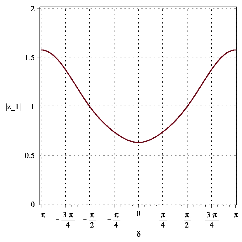
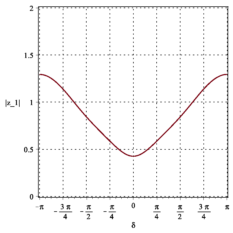
Figure 2: The curves show the ratio of Yukawa couplings in the dominant column $|z_{1}|=|e|/|f|$ as functions of the physical phase $\delta$ evaluated using Eq.51. The left panel is for TBC mixing in Eq.6 while the right panel is for the TBC2 ansatz in Eq.4, both evaluated to second order in $\lambda$. From the left panel we see that $|e|=|f|$ is possible for $\delta\approx\pm\pi/2$ for TBC mixing. From the right panel we see that $|e|/|f|\approx 1/2$ is possible for $\delta\approx 0$ the TBC2 ansatz in Eq.4.

Since we have excluded the possibility of a second texture zero in the previous subsection, here we now consider other types of simple Yukawa coupling patterns, using the “master formula” in Eqs.34-39 combined with the simple (but accurate) parameterisations of mixing angles discussed above, namely TBC in Eq.6 or TBC2 in Eq.4. We first recall the meaning of the ratios $|z_{i}|$ in Eq.54, namely that they correspond to the ratios of magnitudes of Dirac mass matrix elements, or equivalently, Yukawa couplings, and we repeat this result for convenience,

$$|z_{1}|=\frac{|e|}{|f|},\ \ \ \ |z_{2}|=\frac{|b|}{|a|},\ \ \ \ |z_{3}|=\frac{|c|}{|a|}.$$ (104)

These ratios will be calculated in this subsection using Eqs.51-53.

Recall that the ratios of Yukawa couplings in the dominant column, $z_{1}$ in Eq.51, is independent of neutrino masses (and phases) and it only depends on the mixing angles and oscillation phase. In Fig.2 we see that $|z_{1}|=1$ or $|z_{1}|=1/2$ are possible for particular choices of physical phase $\delta$ which depends on the precise values of the mixing angles. From the left panel of Fig.2 we see that for TBC mixing we can achieve

$$|z_{1}|=\frac{|e|}{|f|}=1$$ (105)

for a particular choice of oscillation phase, $\delta=\pm\pi/2$. From the right panel of Fig.2 we see that for TBC2 mixing we can achieve

$$|z_{1}|=\frac{|e|}{|f|}=\frac{1}{2}$$ (106)

for a particular choice of oscillation phase close to zero, $\delta\approx 0$.

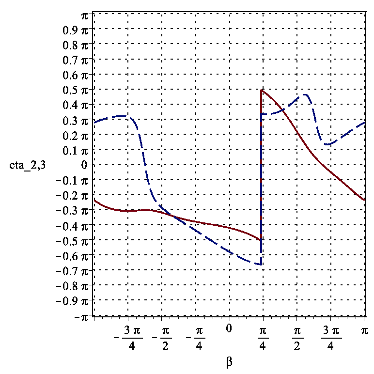
Figure 3: Results for TBC mixing in Eq.6 with $\delta=\pi/2$ and $|z_{1}|=|e|/|f|=1$ as functions of the physical Majorana phase $\beta$. The left panel shows the ratios of Dirac mass matrix elements $|z_{2}|=|b|/|a|$ (solid) and $|z_{3}|=|c|/|a|$ (dashes). The right panel shows the physical phase differences $\eta_{2}=\phi_{b}-\phi_{e}$ (solid) and $\eta_{3}=\phi_{c}-\phi_{f}$ (dashes). Related results may be obtained for $\delta=-\pi/2$ and $|z_{1}|=|e|/|f|=1$.

Mixing	$\delta$	$|z_{1}|$	$\beta$	$|z_{2}|$	$|z_{3}|$	$\eta_{2}$	$\eta_{3}$
TBC	$\pm\pi/2$	1	0	4	4	$\mp 2\pi/5$	$\mp 3\pi/5$
TBC	$\pm\pi/2$	1	$\pm\pi/4$	2	4	$\pm\pi/2$	$\pm\pi/3$
TBC	$\pm\pi/2$	1	$\mp\pi/4$	4	2	$\mp 2\pi/5$	$\mp 2\pi/5$
TBC	$\pm\pi/2$	1	$\pm 3\pi/8$	1	3	$\pm\pi/3$	$\pm\pi/3$
TBC	$\pm\pi/2$	1	$\mp 3\pi/8$	3	1	$\mp\pi/3$	$\mp\pi/3$
TBC	$\pm\pi/2$	1	$\pm\pi/2$	1	2.5	$\pm\pi/5$	$\pm 2\pi/5$
TBC	$\pm\pi/2$	1	$\mp\pi/2$	2.5	1	$\mp\pi/3$	$\mp\pi/3$
TBC	$\pm\pi/2$	1	$\pm 3\pi/4$	1	2	0	$\pm\pi/6$
TBC	$\pm\pi/2$	1	$\mp 3\pi/4$	2	1	$\mp\pi/3$	$\pm\pi/3$
TBC	$\pm\pi/2$	1	$\pm\pi$	2	2	$\mp\pi/5$	$\pm\pi/3$
TBC	$\pm\pi/2$	1	$\mp\pi$	2	2	$\mp\pi/5$	$\pm\pi/3$

Table 1: Examples of simple ratios of Yukawa couplings $|z_{2}|=|b|/|a|$, $|z_{3}|=|c|/|a|$ and corresponding approximate phases as estimated from Fig.3. The exact numerical PMNS parameters for selected cases will be considered later.

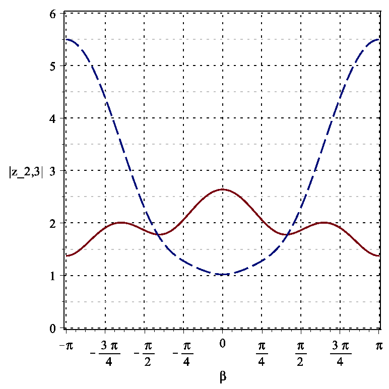
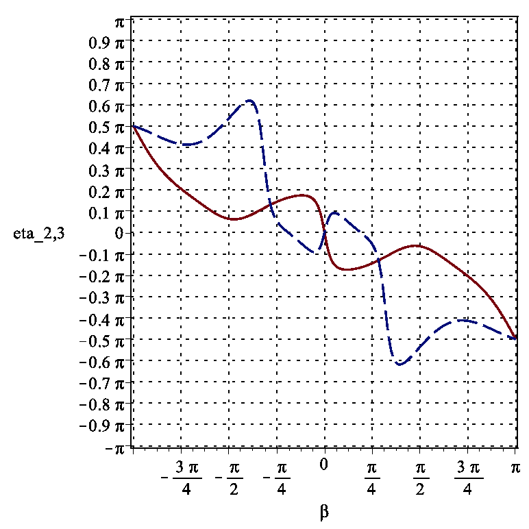
Figure 4: Results for TBC2 mixing in Eq.4 with $\delta=0$ and $|z_{1}|=|e|/|f|=1/2$ as functions of the physical Majorana phase $\beta$. The left panel shows the ratios of Dirac mass matrix elements $|z_{2}|=|b|/|a|$ (solid) and $|z_{3}|=|c|/|a|$ (dashes). The right panel shows the physical phase differences $\eta_{2}=\phi_{b}-\phi_{e}$ (solid) and $\eta_{3}=\phi_{c}-\phi_{f}$ (dashes).

Mixing	$\delta$	$|z_{1}|$	$\beta$	$|z_{2}|$	$|z_{3}|$	$\eta_{2}$	$\eta_{3}$
TBC2	$0$	0.5	$0$	2.5	1	$0$	$0$
TBC2	$0$	0.5	$\pm\pi/4$	2	1	$\mp\pi/6$	$0$
TBC2	$0$	0.5	$\pm\pi/2$	2	2	$0$	$\mp\pi/2$
TBC2	$0$	0.5	$\pm 3\pi/4$	2	4.5	$\mp\pi/5$	$\mp 2\pi/5$
TBC2	$0$	0.5	$\pm\pi$	1.5	5.5	$\mp\pi/2$	$\mp\pi/2$

Table 2: Examples of simple ratios of Yukawa couplings $|z_{2}|=|b|/|a|$, $|z_{3}|=|c|/|a|$ and corresponding approximate phases as estimated from Fig.4. The exact numerical PMNS parameters for selected cases will be considered later.

These are quite interesting results, namely that simple ratios such as $|e|=|f|$ or $|e|/|f|=1/2$ are associated with simple values of oscillation phase, so we shall focus on these two examples.

In the left panel of Fig.3 we show the absolute magnitudes of the ratios $|z_{2}|=|b|/|a|$ and $|z_{3}|=|c|/|a|$ as a function of the Majorana phase $\beta$, for the case of TBC mixing, keeping the oscillation phase fixed at $\delta=\pi/2$ corresponding to $|e|=|f|$ in Eq.105. These ratios concern the second subdominant column of the Dirac mass matrix. As well as simple values of these ratios we are also interested in simple values of the physical phase differences $\eta_{2}=\phi_{b}-\phi_{e}$ and $\eta_{3}=\phi_{c}-\phi_{f}$ and these are shown in the right panel of Fig.3as a function of the Majorana phase $\beta$.

By examining the results in Fig.3 we find some examples of simple ratios of Yukawa couplings in the subdominant column, which are shown together with the phases in Table 1. Analogous results for $\delta=-\pi/2$ are also shown in Table 1, where these results correspond to a symmetry under a change of the sign of all the phases $\delta$, $\beta$, $\eta_{2}$, $\eta_{3}$. This symmetry of the results can be understood by taking the complex conjugate of both sides of the “master formula” in Eq.32. We have verified this symmetry numerically.

Similarly, in the left panel of Fig.4 we show the absolute magnitudes of the ratios $|z_{2}|=|b|/|a|$ and $|z_{3}|=|c|/|a|$ as a function of the Majorana phase $\beta$, for the case of TBC2 mixing, keeping the oscillation phase fixed at $\delta=0$ corresponding to $|e|/|f|=1/2$ in Eq.106. Simple values of the physical phase differences $\eta_{2}=\phi_{b}-\phi_{e}$ and $\eta_{3}=\phi_{c}-\phi_{f}$ are shown in the right panel of Fig.4 as a function of the Majorana phase $\beta$. By examining the results in Fig.4 we find some examples of simple ratios of Yukawa couplings in the subdominant column, which are shown together with the phases in Table 2.

5 Brief Review of Indirect Models

The results in the previous section can be used as the starting point to explore new types of indirect models. Indirect models are fully reviewed in [20] so here we only provide a brief review for completeness.

Indirect models start from simple forms of the Yukawa columns which can be obtained from vacuum alignment due to some discrete non-Abelian family symmetry which is however completely broken. In the class of indirect models, the Klein symmetry of the neutrino mass matrix is not identified as a subgroup of the non-Abelian discrete family symmetry $G$. Models of this class are typically based on the type I seesaw mechanism together with sequential dominance. Here, the main role of the family symmetry consists in relating the Yukawa couplings $e,f$ as well as $a,b,c$ of Eq. 50 by introducing flavon fields which transform as triplets under $G$ (or anti-triplets if the representation is complex) and acquire special vacuum configurations. The directions of the flavon alignments are determined by the $G$ symmetric operators of the flavon potential [20].

Continuing to work in the basis where both the charged leptons as well as the right-handed neutrinos are diagonal, the leptonic flavour structure is encoded in the Dirac neutrino Yukawa operator. The triplet (or anti-triplet) flavons in the neutrino sector denoted $\phi_{\rm atm}$, $\phi_{\rm sol}$ enter linearly as,

$${\cal L}^{\nu}\sim\frac{\phi_{\rm atm}}{\Lambda}\overline{L}N_{\rm atm}H+\frac{\phi_{\rm sol}}{\Lambda}\overline{L}N_{\rm sol}H+M_{\rm atm}\overline{N^{c}}_{\rm atm}N_{\rm atm}+M_{\rm sol}\overline{N^{c}}_{\rm sol}N_{\rm sol}+{H.c}$$ (107)

where $\Lambda$ is a cut-off scale and $H$ is the Standard Model Higgs doublet which is a singlet of $G$, while $L$ are the three lepton doublets which form a triplet representation of $G$. The right-handed neutrinos $N_{\rm atm},N_{\rm sol}$ and the Higgs doublet $H$ are assumed to be in the singlet representation of $G$. However to obtain only the above terms will require additional “shaping symmetries” which we do not specify here ( for examples which also include the charged lepton sector see the review [20]). We obtain the Dirac neutrino Yukawa matrix by inserting the flavon VEVs into Eq. 107. Suppressing the dimensionless couplings of the Dirac neutrino terms for notational clarity, we get

$$Y^{\nu}v~{}=~{}m_{D}~{}=~{}\begin{pmatrix}d&a\\ e&b\\ f&c\end{pmatrix}\equiv\left(\begin{array}[]{cc}m^{D}_{e,\rm atm}&m^{D}_{e,\rm sol}\\ m^{D}_{\mu,\rm atm}&m^{D}_{\mu,\rm sol}\\ m^{D}_{\tau,\rm atm}&m^{D}_{\tau,\rm sol}\end{array}\right)\sim\frac{v}{\Lambda}\begin{pmatrix}\langle\phi_{\rm atm}\rangle_{1}&\langle\phi_{\rm sol}\rangle_{1}\\ \langle\phi_{\rm atm}\rangle_{2}&\langle\phi_{\rm sol}\rangle_{2}\\ \langle\phi_{\rm atm}\rangle_{3}&\langle\phi_{\rm sol}\rangle_{3}\end{pmatrix}.$$ (108)

The columns of the Dirac neutrino Yukawa matrix are therefore proportional to the vacuum alignments of the flavons fields $\phi_{\rm atm}$, $\phi_{\rm sol}$. The effective Majorana operators of the light neutrinos can be derived from this using the seesaw formula of Eq. (16), yielding

$${\cal L}^{\nu}_{eff}~{}\sim~{}\overline{L}\left(\frac{\langle\phi_{\rm atm}\rangle}{\Lambda}\cdot\frac{1}{M_{\rm atm}}\cdot\frac{\langle\phi_{\rm atm}\rangle^{T}}{\Lambda}+\frac{\langle\phi_{\rm sol}\rangle}{\Lambda}\cdot\frac{1}{M_{\rm sol}}\cdot\frac{\langle\phi_{\rm sol}\rangle^{T}}{\Lambda}\right)L^{c}HH,$$ (109)

which has the structure of Eq.11 after the Higgs vev $v$ is inserted. Note that the flavons enter the effective neutrino mass terms quadratically.

In the class of indirect models, the PMNS mixing pattern thus becomes a question of the alignment vectors $\langle\phi_{\rm atm}\rangle$ and $\langle\phi_{\rm sol}\rangle$. For instance, a neutrino mass matrix that gives rise to tri-bimaximal mixing can be obtained using the flavon alignments of constrained sequential dominance (CSD) [25],

$$\frac{\langle\phi_{\rm atm}\rangle}{\Lambda}=\frac{1}{\Lambda}\begin{pmatrix}\langle\phi_{\rm atm}\rangle_{1}\\ \langle\phi_{\rm atm}\rangle_{2}\\ \langle\phi_{\rm atm}\rangle_{3}\end{pmatrix}\propto\begin{pmatrix}0\\ 1\\ 1\end{pmatrix}e^{i\phi_{e}},\qquad\frac{\langle\phi_{\rm sol}\rangle}{\Lambda}=\frac{1}{\Lambda}\begin{pmatrix}\langle\phi_{\rm sol}\rangle_{1}\\ \langle\phi_{\rm sol}\rangle_{2}\\ \langle\phi_{\rm sol}\rangle_{3}\end{pmatrix}\propto\begin{pmatrix}1\\ 1\\ -1\end{pmatrix}e^{i\phi_{b}}.$$ (110)

Note that the resulting columns of the Dirac neutrino Yukawa matrix in Eq.108 are proportional to the columns of the unitary (in the present case TB ) mixing matrix with the physical phase difference $\phi_{b}-\phi_{e}$ being related to the Majorana phase $\beta$. Such a property of the Dirac neutrino Yukawa matrix is generally called form dominance [26]. Furthermore these alignments are left invariant under the action of the Klein symmetry generators, up to an irrelevant sign which drops out due to the quadratic appearance of each flavon. Since the family symmetry $G$ does not contain the neutrino Klein symmetry, its primary role is then to explain the origin of these or similarly simple flavon alignments.

It is clear that CSD is not realistic, primarily because it predicts TB mixing which involves a zero reactor angle. However the above example of CSD does illustrate the general strategy of obtaining simple ratios of Yukawa couplings within a particular column, including the texture zero $d=0$, from vacuum alignment within the framework of indirect models using the techniques reviewed in [20].

An alternative approach to switching on the reactor angle without any “texture zeros” is to consider vacuum alignments which preserve the structure of CSD except that they allow $d\neq 0$, where such models are referred to as partially constrained sequential dominance (PCSD) [28]. The required vacuum alignment has been discussed within an explicit $A_{4}$ model in [29]. With the choice,

$$\frac{\langle\phi_{\rm atm}\rangle}{\Lambda}\propto\begin{pmatrix}re^{i\delta_{0}}\\ 1\\ 1\end{pmatrix}e^{i\phi_{e}},\qquad\frac{\langle\phi_{\rm sol}\rangle}{\Lambda}\propto\begin{pmatrix}1\\ 1\\ -1\end{pmatrix}e^{i\phi_{b}},$$ (111)

one obtains tri-bimaximal-reactor (TBR) mixing, which corresponds to TB mixing but with a non-zero reactor deviation parameter $r$ and an oscillation phase $\delta\approx\delta_{0}$ [28, 29]. For the choice $r=\lambda$ one arrives at TBC mixing [19]. However the main challenge for this approach is to explain why $r=\lambda$, which is not easy to do (for an attempt see [19]).

Another alternative approach is to consider particular alignments with two “texture zeros”. An example of this kind is,

$$\frac{\langle\phi_{\rm atm}\rangle}{\Lambda}\propto\begin{pmatrix}0\\ 1\\ 1\end{pmatrix}e^{i\phi_{e}},\qquad\frac{\langle\phi_{\rm sol}\rangle}{\Lambda}\propto\begin{pmatrix}1\\ 2\\ 0\end{pmatrix}e^{i\phi_{b}}\ \ {\rm or}\ \ \begin{pmatrix}1\\ 0\\ -2\end{pmatrix}e^{i\phi_{b}},$$ (112)

These two alignment possibilities which involve two “texture zeros” were called CSD2 [30]. Note that the above alignments involve the components of each of the flavon alignments $\langle\phi_{\rm atm}\rangle$ and $\langle\phi_{\rm sol}\rangle$ being relatively real. However the overall phase difference between the flavon alignments $\phi_{b}-\phi_{e}$ is physically significant and particular values of this phase difference corresponding to multiples of $\pi/4$ are preferred by the numerical fit resulting in maximal leptonic CP violation [30]. Unfortunately, as we have seen, it is not possible to obtain a large enough reactor angle for the case of a normal neutrino mass hierarchy with two texture zeros. Indeed the reactor angle predicted from CSD2 was $\theta_{13}\approx\frac{\sqrt{2}}{3}\frac{m_{2}}{m_{3}}$ leading to $\theta_{13}\sim 5^{o}-6^{o}$ which is too small [30]. The situation may be improved by considering charged lepton corrections [31], but here we are considering the simple case where such corrections are completely negligible and in this case we cannot have two texture zeros in the two right-handed neutrino case of a normal neutrino mass hierarchy.

Our approach here is to maintain a single “texture zero” $d=0$ which leads to a qualitative understanding of the reactor angle, $\theta_{13}\stackrel{{\scriptstyle<}}{{{}_{\sim}}}m_{2}/m_{3}$. However in order to provide a quantitative understanding of the lepton mixing angles, in the next section we shall consider particular types of vacuum alignment with $\langle\phi_{\rm atm}\rangle_{1}=0$.

6 Searching for New Types of Indirect Models

In the previous subsection we briefly discussed the approaches which already exist in the literature, namely CSD, CSD2 and PCSD, which form the starting point of indirect models. In this section we shall use the results in this paper to explore new approaches which could form the starting point for new indirect models. The new models will involve one single dominant texture zero, as in the case of CSD, and are unlike CSD2 or PCSD which either involve two texture zeros or no texture zeros. However, whereas CSD predicts a zero reactor angle, the new approaches will predict a non-zero reactor angle consistent with experiment.

To obtain realistic solutions which can accommodate the non-zero reactor angle, while maintaining the dominant texture zero $d=\langle\phi_{\rm atm}\rangle_{1}=0$, we shall turn to the results of the previous section based on TBC and TBC2 mixing which are representative of the results from the latest global fits of leptonic mixing angles for the case of a normal neutrino mass hierarchy. From the point of view of Indirect Models we are looking for new examples where the magnitudes of the Yukawa couplings in a particular column occur in simple ratios.

We emphasise that we only use TBC and TBC2 mixing to guide the search for simple alignments since they correspond to two phenomenologically acceptable mixing patterns. We thus allow simple alignments which only approximately satisfy TBC and TBC2 mixing, and may be taken as the starting point for new models, leading to predictions for lepton mixing which do not fit exactly into either of these mixing patterns, but which we expect to be phenomenologically acceptable.

We shall work in a phase basis where the dominant column involves Yukawa couplings which are real and positive, so all the phases occur in the second subdominant column. With this phase convention we can write, the Dirac mass (or Yukawa) matrix, previously given in Eq.99, together with Eq.108, as,

$$\left(\begin{array}[]{cc}0&|a|e^{i\phi_{a}}\\ |e|&|b|e^{i\phi_{b}}\\ |f|&|c|e^{i\phi_{c}}\end{array}\right)\equiv\frac{v}{\Lambda}\begin{pmatrix}0&\langle\phi_{\rm sol}\rangle_{1}\\ \langle\phi_{\rm atm}\rangle_{2}&\langle\phi_{\rm sol}\rangle_{2}\\ \langle\phi_{\rm atm}\rangle_{3}&\langle\phi_{\rm sol}\rangle_{3}\end{pmatrix},$$ (113)

where the phase $\phi_{a}$ is not physical and can always be adjusted to take any value by charged lepton re-phasing, while the two physical phases which are left invariant under charged lepton re-phasing, previously given in Eq.100, in this convention become,

$$\eta_{2}=\phi_{b},\ \ \ \ \eta_{3}=\phi_{c}.$$ (114)

In this convention the flavon alignment $\langle\phi_{\rm atm}\rangle$ is purely real with a zero value in its first component and no phase difference between its second and third components, while the flavon alignment vector $\langle\phi_{\rm sol}\rangle$ may in principle involve three phases, one for each component. Vacuum alignment techniques may lead to an arbitrary phase difference between different aligned components of the same flavon, as in the case of PCSD discussed in Eq.111 where the phase $\delta_{0}$ is undetermined. However it is interesting to look for examples where $\eta_{2}$ and $\eta_{3}$ are are simply related, differing only by a simple rational multiple of $\pi$, since such simple relationships may be later understood in the context of some future theory. One particularly simple example would be where the components $\langle\phi_{\rm sol}\rangle_{1}$, $\langle\phi_{\rm sol}\rangle_{2}$, $\langle\phi_{\rm sol}\rangle_{3}$ are relatively real, i.e. have the same phases up to $\pm\pi$ (remembering that the phase of $\langle\phi_{\rm sol}\rangle_{1}$ is a free choice). An example of this kind of vacuum alignment is CSD2 in Eq.112. A particularly simple example of this kind is,

$$\eta=\eta_{2}=\eta_{3}.$$ (115)

In terms of general flavon models, the overall phases of the different flavon vevs $\langle\phi_{\rm atm}\rangle$ and $\langle\phi_{\rm sol}\rangle$ (i.e. the phases which are factored out of the alignments, for example the remaining phases which appear in CSD in Eq.110 or in CSD2 in Eq.112) are not determined since these overall phases depend on both arbitrary complex Yukawa coupling constants and complex flavon vevs. This is unfortunate since physical mixing angles and CP violating phases depend on this difference of overall phases, as in the example of CSD2 discussed above. However, within special classes of models based on spontaneous CP violation, the Yukawa couplings are constrained to be real and in addition the phases of the overall flavon vevs may be determined using the vacuum alignment techniques discussed in [32]. Within such classes of models the overall phases of $\langle\phi_{\rm atm}\rangle$ and $\langle\phi_{\rm sol}\rangle$ may be determined related in terms of simple rational multiples of $\pi$. Therefore we shall also be interested in such cases.

From Table 1 we find the following phenomenological possibility, corresponding to TBC mixing with $\delta=\pi/2$ and $\beta=-\pi/4$, where this case corresponds to $\eta=\eta_{2}=\eta_{3}=-2\pi/5$, $|z_{1}|=1$, $|z_{2}|=4$, $|z_{3}|=2$. Using Eqs.113 and 114 we can see that this phenomenological example may be used as the basis for constructing a flavon model where the relative phases of the flavons are real, and the overall phases of the flavons take simple values, namely zero and $-2i\pi/5$,

$$\frac{\langle\phi_{\rm atm}\rangle}{\Lambda}\propto\begin{pmatrix}0\\ 1\\ 1\end{pmatrix}\equiv A,\qquad\frac{\langle\phi_{\rm sol}\rangle}{\Lambda}\propto\begin{pmatrix}1\\ 4\\ 2\end{pmatrix}e^{-2i\pi/5}\equiv B,$$ (116)

where we have used the phase freedom in $\phi_{a}$ to set this phase equal to $-2\pi/5$.

The alignments defined as $A$ and $B$ above are not sufficient to determine the effective neutrino mass matrix and hence the PMNS mixing parameters. Their normalisation is also required. In the case of form dominance, the alignments would be sufficient to determine the PMNS mixing parameters but form dominance is not satisfied. The effective neutrino mass matrix can be written as,

$$m^{\nu}=m_{a}A^{T}A+m_{b}B^{T}B=m_{a}A^{T}A+m_{a}\epsilon_{\nu}B^{T}B$$ (117)

where $m_{a}$ and $m_{b}$ are real mass parameters which determine the physical neutrino masses $m_{3}$ and $m_{2}$. For fixed alignments $A,B$, the ratio $\epsilon_{\nu}=m_{b}/m_{a}$ will also affect the PMNS mixing parameters. For the above alignment this ratio is given by,

$$\epsilon_{\nu}=\left(\frac{1}{4}\frac{|\tilde{b}|}{|\tilde{e}|}\right)^{2},$$ (118)

where this ratio is related to physical parameters using Eqs.40-43. For the case of TBC mixing with $\delta=\pi/2$ and $\beta=-\pi/4$, with the mass ratio as in Eq.64, we find numerically that

$$\frac{|\tilde{b}|}{|\tilde{e}|}=0.9159.$$ (119)

This completely fixes the neutrino mass matrix up to an overall scale $m_{a}$ which does not affect the PMNS mixing parameters. Using the Mixing Parameter Tools (MPT) package associated with [33] , we can check the predictions of this vacuum alignment, which may be compared to the original mixing pattern that was assumed to derive it (in brackets). For example, using the above alignment with $\epsilon_{\nu}=0.058$ we find using MPT, $m_{2}/m_{3}=0.17$ together with,

$$\theta_{12}=34.2^{o},\ \ \theta_{13}=9.2^{o},\ \ \theta_{23}=40.9^{o},\ \ \delta=107^{o},\ \ \beta=-83^{o},$$ (120)

which is in good agreement with the global fits. The discrepancy between Eqs.120 and the TBC mixing angles in Eq.5 arises due to the approximation in setting the ratios $|z_{i}|$ and the phases $\eta_{i}$ equal to simple values. We have checked that using the accurate values of the alignments, obtained from the master formula in Eq.32, with the ratios of Yukawa couplings calculated using Eqs.51, 52, 65 and the phases calculated using Eq.100 together with Eqs.101,102,103, namely:

$$A\equiv\begin{pmatrix}0\\ 1\\ 1\end{pmatrix},\qquad B\equiv\begin{pmatrix}1\\ 3.725e^{-i\pi 0.373}\\ 2.028e^{-i\pi 0.479}\end{pmatrix},$$ (121)

with

$$\epsilon_{\nu}=\left(\frac{1}{3.725}\frac{|\tilde{b}|}{|\tilde{e}|}\right)^{2}=0.06045,$$ (122)

when used in Eq.117 reproduce the TBC angles in Eq.5 to excellent accuracy. This gives us confidence that the master formula and the procedure that we followed to obtain the Yukawa ratios and the phases is correct. It also supports our approach of using the values obtained in Table 1 and Table 2 as the starting point for new simple but approximate alignments, which lead to phenomenologically viable possibilities which differ from either TBC or TBC2 mixing which were used to discover the new alignments, but which can subsequently be discarded. Thus the alignment in Eq.121 which reproduces TBC mixing is discarded in favour of the approximate but simpler alignment in Eq.116 which gives the different but phenomenologically viable mixing in Eq.120.

As a second example from Table 1 we find the following phenomenological possibility, corresponding to approximate TBC mixing with $\delta=\pi/2$ and $\beta=3\pi/8$, where this case corresponds to $\eta=\eta_{2}=\eta_{3}=\pi/3$, $|z_{1}|=1$, $|z_{2}|=1$, $|z_{3}|=3$. This suggests the alignments, in our phase convention,

$$A\equiv\begin{pmatrix}0\\ 1\\ 1\end{pmatrix},\qquad B\equiv\begin{pmatrix}1\\ 1\\ 3\end{pmatrix}e^{i\pi/3}.$$ (123)

In a realistic model, the alignments may be predicted by some family symmetry for example, but not the value of $\epsilon_{\nu}$ which will depend on right-handed neutrino masses and unknown Yukawa couplings. Therefore we shall regard $\epsilon_{\nu}$ as a free parameter which may be varied to give different the correct ratio of physical neutrino masses $m_{2}/m_{3}$. For example, using the above alignment with $\epsilon_{\nu}=0.1$ we find using MPT, $m_{2}/m_{3}=0.17$ together with,

$$\theta_{12}=34.3^{o},\ \ \theta_{13}=8.6^{o},\ \ \theta_{23}=44.3^{o},\ \ \delta=93^{o},\ \ \beta=72^{o},$$ (124)

which is in good agreement with the global fits.

As a third example from Table 1 we find the following phenomenological possibility, corresponding to approximate TBC mixing with $\delta=\pi/2$ and $\beta=-3\pi/8$, where this case corresponds to $\eta=\eta_{2}=\eta_{3}=-\pi/3$, $|z_{1}|=1$, $|z_{2}|=3$, $|z_{3}|=1$. This suggests the alignments, in our phase convention,

$$A\equiv\begin{pmatrix}0\\ 1\\ 1\end{pmatrix},\qquad B\equiv\begin{pmatrix}1\\ 3\\ 1\end{pmatrix}e^{-i\pi/3}.$$ (125)

For example, using the above alignment with $\epsilon_{\nu}=0.1$ we find using MPT, $m_{2}/m_{3}=0.17$ together with,

$$\theta_{12}=34.3^{o},\ \ \theta_{13}=8.6^{o},\ \ \theta_{23}=45.7^{o},\ \ \delta=87^{o},\ \ \beta=-72^{o},$$ (126)

which again is in good agreement with the global fits.

We emphasise that, with the alignments including the phase $\eta$ fixed, the neutrino mass matrix is completely determined by only two parameters in Eq.117, namely an overall mass scale $m_{a}$, which may be taken to fix the atmospheric neutrino mass $m_{3}=0.048-0.051$ eV, the ratio of input masses $\epsilon_{\nu}$, which may be taken to fix the solar to atmospheric neutrino mass ratio $m_{2}/m_{3}=0.17-0.18$. In particular the entire PMNS mixing matrix and all the parameters therein are then predicted as a function of $m_{2}/m_{3}$ controlled by the only remaining parameter $\epsilon_{\nu}$. In Table 3 we show the predictions for the first example above in Eq.116 as a function of $\epsilon_{\nu}$ and hence $m_{2}/m_{3}$. In Table 4 we show the predictions for the second example above in Eq.123 as a function of $\epsilon_{\nu}$ and hence $m_{2}/m_{3}$. In Table 5 we show the predictions for the third example above in Eq.125 as a function of $\epsilon_{\nu}$ and hence $m_{2}/m_{3}$. The results in Table 4 and Table 5 only differ in the atmospheric angle and the oscillation phase $\delta$, which are correlated via an atmospheric sum rule discussed later in Eq.184, with both sets of results approximated by TBC mixing to within an accuracy of one degree, but with the phases predicted.

We remark that an accuracy of one degree in the angles is all that can be expected due to purely theoretical corrections in a realistic model due to renormalisation group running [34] and canonical normalisation corrections [35]. In addition, there may be small contributions from a heavy third right-handed neutrino [36] which can affect the results.

$\epsilon_{\nu}$	$m_{2}/m_{3}$	$\theta_{12}$	$\theta_{13}$	$\theta_{23}$	$\delta$	$\beta$
0.057	0.166	34.2∘	9.0∘	40.8∘	107∘	-84∘
0.058	0.170	34.2∘	9.2∘	40.9∘	107∘	-83∘
0.059	0.174	34.1∘	9.4∘	41.0∘	106∘	-82∘
0.060	0.177	34.1∘	9.6∘	41.1∘	105∘	-80∘
0.061	0.181	34.1∘	9.7∘	41.3∘	104∘	-79∘

Table 3: The predictions for PMNS parameters and $m_{2}/m_{3}$ arising from Eq.116 as a function of $\epsilon_{\nu}$. Note that these predictions assume $\eta=-2\pi/5$. Identical results are obtained for $\eta=2\pi/5$ with the phases $\beta$ and $\delta$ changed in sign.

$\epsilon_{\nu}$	$m_{2}/m_{3}$	$\theta_{12}$	$\theta_{13}$	$\theta_{23}$	$\delta$	$\beta$
0.098	0.168	34.4∘	8.4∘	44.4∘	92∘	-73∘
0.100	0.171	34.3∘	8.6∘	44.3∘	93∘	-72∘
0.102	0.173	34.3∘	8.75∘	44.1∘	94∘	-71∘
0.104	0.177	34.3∘	8.9∘	44.0∘	94∘	-70∘
0.106	0.179	34.2∘	9.1∘	43.8∘	95∘	-69∘

Table 4: The predictions for PMNS parameters and $m_{2}/m_{3}$ arising from CSD3 in Eq.123 as a function of $\epsilon_{\nu}$. Note that these predictions assume $\eta=\pi/3$. Identical results are obtained for $\eta=-\pi/3$ with the phases $\beta$ and $\delta$ changed in sign. These angle predictions are approximately equal to the Tri-bimaximal-Cabibbo mixing angle values $\theta_{12}=35.26^{\circ}$, $\theta_{13}=9.15^{\circ}$, $\theta_{23}=45^{\circ}$ to within one degree.

$\epsilon_{\nu}$	$m_{2}/m_{3}$	$\theta_{12}$	$\theta_{13}$	$\theta_{23}$	$\delta$	$\beta$
0.098	0.168	34.4∘	8.4∘	45.5∘	88∘	-73∘
0.100	0.171	34.3∘	8.6∘	45.7∘	87∘	-72∘
0.102	0.173	34.3∘	8.75∘	45.9∘	86∘	-71∘
0.104	0.177	34.3∘	8.9∘	46.0∘	86∘	-70∘
0.106	0.179	34.2∘	9.1∘	46.2∘	85∘	-69∘

Table 5: The predictions for PMNS parameters and $m_{2}/m_{3}$ arising from CSD3 in Eq.125 as a function of $\epsilon_{\nu}$. Note that these predictions assume $\eta=-\pi/3$. Identical results are obtained for $\eta=\pi/3$ with the phases $\beta$ and $\delta$ changed in sign. These angle predictions are approximately equal to the Tri-bimaximal-Cabibbo mixing angle values $\theta_{12}=35.26^{\circ}$, $\theta_{13}=9.15^{\circ}$, $\theta_{23}=45^{\circ}$ to within one degree.

7 Leading Order Analytic Results

The above results are numerical, based on the exact analytic master formula in Eq.32. In order to get some feeling for the results it is worth taking a look at the well known but approximate analytic expressions for the masses and mixing parameters in terms of the Dirac mass matrix elements and right-handed neutrino masses, bearing in mind that these results may have large corrections. The neutrino masses in terms of the parameters in Eq.14 are given to leading order in $m_{2}/m_{3}$ by [7, 10],

$$m_{1} = 0$$ (127)

$$m_{2} \approx \frac{|a|^{2}}{Xs_{12}^{2}}$$ (128)

$$m_{3} \approx \frac{|e|^{2}+|f|^{2}}{Y}$$ (129)

The neutrino mixing angles are given to leading order in $m_{2}/m_{3}$ by [7, 10],

$$\tan\theta_{23} \approx \frac{|e|}{|f|}$$ (130)

$$\tan\theta_{12} \approx \frac{|a|}{c_{23}|b|\cos(\tilde{\phi}_{b})-s_{23}|c|\cos(\tilde{\phi}_{c})}$$ (131)

$$\theta_{13} \approx e^{i(\tilde{\phi}+\phi_{a}-\phi_{e})}\frac{|a|(e^{*}b+f^{*}c)}{[|e|^{2}+|f|^{2}]^{3/2}}\frac{Y}{X}$$ (132)

where we have written some (but not all) complex Yukawa couplings as $x=|x|e^{i\phi_{x}}$. The Dirac CP violating oscillation phase $\delta$ is fixed to give a real angle $\theta_{12}$ by,

$$c_{23}|b|\sin(\tilde{\phi}_{b})\approx s_{23}|c|\sin(\tilde{\phi}_{c})$$ (133)

where

$$\tilde{\phi}_{b} \equiv \phi_{b}-\phi_{a}-\tilde{\phi}+\delta,$$

$$\tilde{\phi}_{c} \equiv \phi_{c}-\phi_{a}+\phi_{e}-\phi_{f}-\tilde{\phi}+\delta$$ (134)

The phase $\tilde{\phi}$ is fixed to give a real angle $\theta_{13}$ by [7],

$$\tilde{\phi}\approx\phi_{e}-\phi_{a}-\phi$$ (135)

where

$$\phi=\arg(e^{*}b+f^{*}c).$$ (136)

Eq.136 may be expressed as

$$\tan\phi\approx\frac{|b|s_{23}s_{2}+|c|c_{23}s_{3}}{|b|s_{23}c_{2}+|c|c_{23}c_{3}}.$$ (137)

Inserting $\tilde{\phi}$ in Eq.135 into Eqs.133,134, we obtain,

$$\tan(\phi+\delta)\approx\frac{|b|c_{23}s_{2}-|c|s_{23}s_{3}}{-|b|c_{23}c_{2}+|c|s_{23}c_{3}}$$ (138)

where we have written $s_{i}=\sin\eta_{i},c_{i}=\cos\eta_{i}$ where

$$\eta_{2}\equiv\phi_{b}-\phi_{e},\ \ \eta_{3}\equiv\phi_{c}-\phi_{f}$$ (139)

are the phases introduced in Eq.100 which are invariant under a charged lepton phase transformation. The reason that the see-saw parameters only involve two invariant phases $\eta_{2},\eta_{3}$ rather than the usual six is due to the two-right handed neutrino assumption, which removes three phases, together with the assumption of a dominant texture zero, which removes another phase.

From the above approximate leading order results we find the following alternative useful expressions for the mixing angles,

$$\tan\theta_{23} \approx |z_{1}|$$ (140)

$$\cot\theta_{12} \approx c_{23}|z_{2}|\cos\left(\eta_{2}-\frac{\beta}{2}\right)-s_{23}|z_{3}|\cos\left(\eta_{3}-\frac{\beta}{2}\right)$$ (141)

$$\theta_{13} \approx \frac{m_{2}}{m_{3}}s_{12}^{2}c_{23}\left||z_{3}|+|z_{2}|\tan\theta_{23}e^{i(\eta_{2}-\eta_{3})}\right|$$ (142)

where $\eta_{2}$ and $\eta_{3}$ are given in Eq.100 and $|z_{i}|$ are given in Eq.104. The above approximate leading order results should be compared to the exact results in Eqs.51-53. In fact they may be derived by inverting Eqs.51-53. This is non-trivial to do exactly, but to leading order in $m_{2}/m_{3}$ it leads to the results in Eqs.140-142, using the standard PDG expressions for the mixing elements. We emphasise that these leading order results are very crude, for example we have seen from Fig.2 that for close to maximal mixing $z_{1}\approx 1$ has a 50% variation depending on the phase $\delta$. Indeed maximal atmospheric mixing prefers $\delta\approx\pi/2$. This is due to next to leading order effects beyond the simple approximations above. However the leading order results do provide some understanding of the successful alignments discussed in the previous subsection as we now discuss.

The alignments discussed in the previous subsection have $\eta=\eta_{2}=\eta_{3}$ and lead to approximate maximal mixing with $|z_{1}|=1$ and $\tan\theta_{23}\approx 1$. In this case the approximate formulas above become,

$$\cot\theta_{12} \approx \frac{1}{\sqrt{2}}\cos\left(\eta-\frac{\beta}{2}\right)(|z_{2}|-|z_{3}|)$$ (143)

$$\theta_{13} \approx \frac{s_{12}^{2}}{\sqrt{2}}\frac{m_{2}}{m_{3}}(|z_{3}|+|z_{2}|).$$ (144)

These approximate results show that the solar angle depends on the difference between $|z_{2}|$ and $|z_{3}|$ and the phase difference $\eta-\frac{\beta}{2}$. Phenomenologically we must arrange to obtain $\cot\theta_{12}\approx\sqrt{2}$ leading to the approximate condition for the difference,

$$|z_{2}|-|z_{3}| \approx \frac{2}{\cos(\eta-\frac{\beta}{2})}$$ (145)

Since $s_{12}^{2}\approx 1/3$ the reactor angle is approximately given by,

$$\theta_{13} \approx \frac{1}{3\sqrt{2}}\frac{m_{2}}{m_{3}}(|z_{2}|+|z_{3}|).$$ (146)

Since phenomenologically ${m_{2}}/{m_{3}}\approx\lambda/\sqrt{2}$ and $\theta_{13}\approx\lambda/\sqrt{2}$, we obtain the approximate condition for the sum,

$$|z_{2}|+|z_{3}|\approx 3\sqrt{2}.$$ (147)

In the examples where $\eta=\eta_{2}=\eta_{3}$, there is only a single see-saw phase $\eta$ and so all physical phases must be related to it. In particular we find, using the above results and other approximate results for the phases in [7, 10] that, for $|z_{2}|>|z_{3}|$, $\phi=\eta$ and $\delta\approx-2\eta$ and $\beta\approx 2\eta$. Thus the Majorana phase $\beta$ is simply related to the oscillation phase $\delta$ according to $\delta\approx-\beta$. From Eq.145 we find in these cases,

$$|z_{2}|-|z_{3}| \approx 2.$$ (148)

Solving Eqs.147 and 148 we find,

$$|z_{2}|\approx\frac{3}{\sqrt{2}}+1\approx 3.1,\ \ |z_{3}|\approx\frac{3}{\sqrt{2}}-1\approx 1.1.$$ (149)

These results are well respected by the third example in Eq.125 corresponding to $|z_{1}|=1$, $|z_{2}|=3$, $|z_{3}|=1$. For the second example analogous results to those in Eq.149 may be derived but with $|z_{2}|$ and $|z_{3}|$ being interchanged, which is in good agreement with $|z_{2}|=1$, $|z_{3}|=3$. The first example in Eq.116 with $|z_{1}|=1$, $|z_{2}|=4$, $|z_{3}|=2$ does not obey the estimate in Eq.149 very well. Nevertheless it leads to good agreement with experiment, which highlights the limitations of the leading order results, and the importance of the exact master formula.

8 Link between Leptogenesis and PMNS phases

In the two right-handed neutrino model with dominant texture zero, that we are considering in this paper, Eq.114 shows that there are only two see-saw phases that are relevant, namely $\eta_{2}$ and $\eta_{3}$. The low energy PMNS phases $\delta$ and $\beta$ are therefore (complicated) functions of these two see-saw phases, and the other see-saw parameters, with the exact relation obtained via the master formula in Eq.32. The phases relevant for leptogenesis can also only depend on the two see-saw phases $\eta_{2}$ and $\eta_{3}$. This implies that the phases which control leptogenesis must be related to the two physical low energy PMNS phases $\delta$ and $\beta$. This means that by studying CP violation in the laboratory one is in fact also probing CP violation in the early universe which was relevant for matter-antimatter asymmetry.

The Leptogenesis-PMNS link for the two right-handed neutrino model with dominant texture zero been discussed some time ago in the literature, first for flavour independent leptogenesis in [10], then later for flavour dependent leptogenesis in [37]. In the flavour independent leptogenesis case [10] the lepton asymmetry is proportional to $\sin 2\phi$ where the relevant leptogenesis phase is $\phi$ was defined in Eq.136. In the flavour dependent leptogenesis case [37] muon-type lepton asymmetry is proportional to $\sin(\phi+\eta_{2})$, with tau-type lepton asymmetry being proportional to $\sin(\phi+\eta_{3})$ and electron-type lepton asymmetry being identically zero due to the texture zero.

Estimates of the baryon asymmetry $Y_{B}$, including the effects of washout, for the case where the lightest right-handed neutrino dominates the production of baryon asymmetry (so-called $N_{1}$ leptogenesis) for the flavour-dependent case were made in [37], in particular for the above case of the two right-handed neutrino model with a dominant texture zero. When the lightest right-handed neutrino is identified with $N_{\rm atm}$, one finds [37], assuming $|e|\approx|f|$ which leads to equal washouts $\eta_{\mu}\approx\eta_{\tau}$,

$$Y_{B}\propto|b|\sin(\phi+\eta_{2})+|c|\sin(\phi+\eta_{3}).$$ (150)

When the lightest right-handed neutrino is identified with $N_{\rm sol}$, one finds [37], assuming $|e|\approx|f|$, with unequal washouts in this case,

$$Y_{B}\propto-\eta_{\mu}|b|\sin(\phi+\eta_{2})-\eta_{\tau}|c|\sin(\phi+\eta_{3}).$$ (151)

The above estimates assume that the lightest right-handed neutrino dominates the production of baryon asymmetry ($N_{1}$ leptogenesis). In certain situations the heavier right-handed neutrino can dominate ($N_{2}$ leptogenesis) as was discussed for the two right-handed neutrino model, especially for the case where the lightest right-handed neutrino is identified with $N_{\rm atm}$ [38]. In this case the situation is more involved, and it is not possible to give simple analytic estimates for the baryon asymmetry as above. However we remark that for $N_{2}$ leptogenesis the flavour dependent lepton asymmetries are proportional to the same phase factors as for $N_{1}$ leptogenesis but have opposite sign.

For the examples where $\eta=\eta_{2}=\eta_{3}$ the baryon asymmetry $Y_{B}$ is clearly proportional to a common factor $\sin(\phi+\eta)$. From Eq.136 we see that in this case $\phi=\eta$ which is an exact result. Hence the baryon asymmetry is proportional to $\sin(2\eta)$ or $\sin(2\phi)$ which makes sense since $\eta$ is the only remaining see-saw phase in this case. The physical low energy CP violating phases $\beta$ and $\delta$ must vanish in the limit that $\eta\rightarrow 0$ since $\eta$ is the only high energy source of CP violation at the see-saw scale. The exact relationship between $\beta,\delta$ and $\eta$ provided via the master formula is rather complicated, however the leading order estimates for the phases derived from [7, 10] are $\delta\approx-2\eta$ and $\beta\approx 2\eta$, which are in fair agreement with the numerical results in Eq.126. Thus, approximately, we have in this case that the lepton asymmetry is proportional to $\sin\delta$, which is maximal in this case. The main message is that, by studying CP violation in oscillation experiments, one is in fact also probing the source of CP violation in the early universe which was relevant for matter-antimatter asymmetry.

9 A Minimal Predictive See-Saw Model

9.1 CSD3 and vacuum alignment

In discussing the implications of our results for model building, we have been guided by the idea that the most attractive flavon alignments are the simplest ones, since they may eventually arise from some realistic model. Although we have tabulated several relatively simple possibilities, we have only explored three examples from Table 1 in detail. These three examples all satisfy the conditions that $\eta\equiv\eta_{2}=\eta_{3}$ so that the components of a given flavon all carry the same phase and lead to approximate maximal mixing with $|z_{1}|=1$ which means that the atmospheric flavon alignment is particularly simple and retains the CSD form in Eq.110. However the price of the non-zero reactor angle (at least in our minimal approach where we maintain the zero in the atmospheric vacuum alignment, and do not invoke charged lepton corrections) is that the solar flavon alignment must differ from the CSD alignment shown in Eq.110, and in general will be more complicated. The question then arises as to whether such alignments may be achieved theoretically from vacuum alignment methods.

In this subsection we shall discuss two of the successful flavon alignments which we have discovered in our general analysis, and show how they may be derived from vacuum alignment methods. The two examples we shall consider (which correspond to the second and third examples discussed earlier in this section) are summarised below,

$$\frac{\langle\phi_{\rm atm}\rangle}{\Lambda}\propto\begin{pmatrix}0\\ 1\\ 1\end{pmatrix}e^{i\phi_{e}},\qquad\frac{\langle\phi_{\rm sol}\rangle}{\Lambda}\propto\begin{pmatrix}1\\ 1\\ 3\end{pmatrix}e^{i\phi_{b}}\ \ {\rm or}\ \ \begin{pmatrix}1\\ 3\\ 1\end{pmatrix}e^{i\phi_{b}},$$ (152)

These two new alignment possibilities shall both be referred to as CSD3, since they both represent new possibilities not considered before in the literature. As in the case of CSD2 [30] the above alignments involve the components of each of the flavon alignments $\langle\phi_{\rm atm}\rangle$ and $\langle\phi_{\rm sol}\rangle$ being relatively real within each flavon, although the overall phase of that flavon will in general be non-zero. However the overall phase difference between the flavon alignments $\eta=\phi_{b}-\phi_{e}$ is physically significant and we have seen that particular values of this phase difference are preferred. In a particular phase convention, the preferred values are displayed in Eqs.123 and 125.

The vacuum alignments associated with TB mixing have been very well studied. Here we shall focus on the family symmetry $A_{4}$ as it is the smallest non-Abelian finite group with an irreducible triplet representation. We apply the $A_{4}$ basis in which the triplets are explicitly real as given for example in [39]. We shall work in the basis of [29] where, denoting a general $A_{4}$ triplet as ${\bf{c}}=(c_{1},c_{2},c_{3})^{T}$ and defining $\omega=e^{2\pi i/3}$, the product rules can be summarised as

$${\bf{c\otimes c^{\prime}}}~{}=~{}\sum_{r=0}^{2}(c_{1}c^{\prime}_{1}+\omega^{-r}c_{2}c^{\prime}_{2}+\omega^{r}c_{3}c^{\prime}_{3})\;+\,\begin{pmatrix}c_{2}c^{\prime}_{3}\\ c_{3}c^{\prime}_{1}\\ c_{1}c^{\prime}_{2}\end{pmatrix}+\begin{pmatrix}c_{3}c^{\prime}_{2}\\ c_{1}c^{\prime}_{3}\\ c_{2}c^{\prime}_{1}\end{pmatrix}\ ,$$ (153)

corresponding to two triplets and the sum of the three one-dimensional irreducible representations ${\bf{1_{r}}}$, with ${\bf{1_{0}=1}}$ being the trivial singlet.

Following the methods of [29] it is straightforward to obtain the vacuum alignments for charged lepton flavon alignments suitable for a diagonal charged lepton mass matrix. The charged lepton flavon alignments used to generate a diagonal charged lepton mass matrix are obtained from the renormalisable superpotential [29],

$$W_{A_{4}}^{\mathrm{flavon},\ell}~{}\sim~{}A_{e}\varphi_{e}\varphi_{e}+A_{\mu}\varphi_{\mu}\varphi_{\mu}+A_{\tau}\varphi_{\tau}\varphi_{\tau}+O_{e\mu}\varphi_{e}\varphi_{\mu}+O_{e\tau}\varphi_{e}\varphi_{\tau}+O_{\mu\tau}\varphi_{\mu}\varphi_{\tau}\ .$$ (154)

The triplet driving fields $A_{e,\mu,\tau}$ give rise to flavon alignments $\langle\varphi_{e,\mu,\tau}\rangle$ with two zero components, and the singlet driving fields $O_{ij}$ require orthogonality among the three flavon VEVs so that we arrive at the vacuum structure [29],

$$\langle\varphi_{e}\rangle=v_{e}\begin{pmatrix}1\\ 0\\ 0\end{pmatrix}\ ,\qquad\langle\varphi_{\mu}\rangle=v_{\mu}\begin{pmatrix}0\\ 1\\ 0\end{pmatrix}\ ,\qquad\langle\varphi_{\tau}\rangle=v_{\tau}\begin{pmatrix}0\\ 0\\ 1\end{pmatrix}\ .$$ (155)

Of more interest to us in this paper are the new neutrino flavon alignments. The starting point for the discussion is the usual standard TB neutrino flavon alignments proportional to the respective columns of the TB mixing matrix,

$$\langle\varphi_{\nu_{1}}\rangle=v_{\nu_{1}}\begin{pmatrix}2\\ -1\\ 1\end{pmatrix},\qquad\langle\varphi_{\nu_{2}}\rangle=v_{\nu_{2}}\begin{pmatrix}1\\ 1\\ -1\end{pmatrix},\qquad\langle\varphi_{\nu_{3}}\rangle=v_{\nu_{3}}\begin{pmatrix}0\\ 1\\ 1\end{pmatrix}.$$ (156)

In the remainder of this subsection we shall show how to obtain the neutrino flavon alignments including the new alignment,

$$\langle\varphi_{\nu_{4}}\rangle=v_{\nu_{4}}\begin{pmatrix}1\\ 3\\ 1\end{pmatrix},$$ (157)

which is an example of a CSD3 solar flavon alignment in Eq.152. In constructing a CSD3 model in the notation of Eq.152 we shall identify $\phi_{\rm atm}\equiv\varphi_{\nu_{3}}$, and $\phi_{\rm sol}\equiv\varphi_{\nu_{4}}$. The renormalisable superpotential involving the driving fields necessary for aligning the neutrino-type flavons is given as

$$W_{A_{4}}^{\mathrm{flavon},\nu} = A_{\nu_{2}}(g_{1}\varphi_{\nu_{2}}\varphi_{\nu_{2}}+g_{2}\varphi_{\nu_{2}}\xi_{\nu_{2}})$$

$$+\,O_{e\nu_{3}}g_{3}\varphi_{e}\varphi_{\nu_{3}}+O_{\nu_{2}\nu_{3}}g_{4}\varphi_{\nu_{2}}\varphi_{\nu_{3}}+O_{\nu_{1}\nu_{2}}g_{5}\varphi_{\nu_{1}}\varphi_{\nu_{2}}+O_{\nu_{1}\nu_{3}}g_{6}\varphi_{\nu_{1}}\varphi_{\nu_{3}}$$

$$+\,O_{\mu\nu_{5}}g_{7}\varphi_{\mu}\varphi_{\nu_{5}}+O_{\nu_{2}\nu_{5}}g_{8}\varphi_{\nu_{2}}\varphi_{\nu_{5}}+O_{\mu{\nu_{6}}}g_{9}\varphi_{\mu}\varphi_{\nu_{6}}+O_{{\nu_{5}}{\nu_{6}}}g_{10}\varphi_{\nu_{5}}\varphi_{\nu_{6}}$$

$$+\,O_{{\nu_{6}}\nu_{4}}g_{11}\varphi_{\nu_{6}}\varphi_{\nu_{4}}+\,O_{\nu_{1}\nu_{4}}g_{12}\varphi_{\nu_{1}}\varphi_{\nu_{4}},$$

where $A_{\nu_{2}}$ is a triplet driving field and $O_{ij}$ are singlet driving fields whose F-terms lead to orthogonality relations between the accompanying flavon fields. Here $g_{i}$ are dimensionless coupling constants. The first line of Eq. (9.1) produces the vacuum alignment $\langle\varphi_{\nu_{2}}\rangle\propto(1,1,-1)^{T}$ of Eq. (156) as can be seen from the $F$-term conditions

$$2g_{1}\begin{pmatrix}\langle\varphi_{\nu_{2}}\rangle_{2}\langle\varphi_{\nu_{2}}\rangle_{3}\\ \langle\varphi_{\nu_{2}}\rangle_{3}\langle\varphi_{\nu_{2}}\rangle_{1}\\ \langle\varphi_{\nu_{2}}\rangle_{1}\langle\varphi_{\nu_{2}}\rangle_{2}\end{pmatrix}+g_{2}\langle\xi_{\nu_{2}}\rangle\begin{pmatrix}\langle\varphi_{\nu_{2}}\rangle_{1}\\ \langle\varphi_{\nu_{2}}\rangle_{2}\\ \langle\varphi_{\nu_{2}}\rangle_{3}\end{pmatrix}~{}=~{}\begin{pmatrix}0\\ 0\\ 0\end{pmatrix}.$$ (159)

The first two terms in the second line of Eq. (9.1) give rise to orthogonality conditions which uniquely fix the alignment $\langle\varphi_{\nu_{3}}\rangle\propto(0,1,1)^{T}$ of Eq. (156),

$$\langle\varphi_{e}\rangle^{T}\cdot\langle\varphi_{\nu_{3}}\rangle\,=\,\langle\varphi_{\nu_{2}}\rangle^{T}\cdot\langle\varphi_{\nu_{3}}\rangle\,=\,0\quad \rightarrow \quad\langle\varphi_{\nu_{3}}\rangle\,\propto\,\begin{pmatrix}0\\ 1\\ 1\end{pmatrix}\ .$$ (160)

The last two terms in the second line of Eq. (9.1) give rise to orthogonality conditions which uniquely fix the alignment $\langle\varphi_{\nu_{1}}\rangle\propto(2,-1,1)^{T}$ of Eq. (156),

$$\langle\varphi_{\nu_{1}}\rangle^{T}\cdot\langle\varphi_{\nu_{2}}\rangle\,=\,\langle\varphi_{\nu_{1}}\rangle^{T}\cdot\langle\varphi_{\nu_{3}}\rangle\,=\,0\quad \rightarrow \quad\langle\varphi_{\nu_{1}}\rangle\,\propto\,\begin{pmatrix}2\\ -1\\ 1\end{pmatrix}\ .$$ (161)

The terms in the third line of Eq. (9.1) give rise to orthogonality conditions which uniquely fix the alignments of the auxiliary flavon fields $\varphi_{\nu_{5}}$ and $\varphi_{\nu_{6}}$,

$$\langle\varphi_{\mu}\rangle^{T}\cdot\langle\varphi_{\nu_{5}}\rangle\,=\,\langle\varphi_{\nu_{2}}\rangle^{T}\cdot\langle\varphi_{\nu_{5}}\rangle\,=\,0\quad \rightarrow \quad\langle\varphi_{\nu_{5}}\rangle\,\propto\,\begin{pmatrix}1\\ 0\\ 1\end{pmatrix}\ ,$$ (162)

$$\langle\varphi_{\mu}\rangle^{T}\cdot\langle\varphi_{\nu_{6}}\rangle\,=\,\langle\varphi_{\nu_{5}}\rangle^{T}\cdot\langle\varphi_{\nu_{6}}\rangle\,=\,0\quad \rightarrow \quad\langle\varphi_{\nu_{6}}\rangle\,\propto\,\begin{pmatrix}1\\ 0\\ -1\end{pmatrix}\ .$$ (163)

The neutrino-type flavon of interest labelled as $\varphi_{\nu_{4}}$ gets aligned by the remaining terms in the fourth line of Eq. (9.1). A vanishing $F$-term of the driving field $O_{{\nu_{6}}\nu_{4}}$ requires

$$\langle\varphi_{\nu_{4}}\rangle=\begin{pmatrix}n_{1}\\ n_{2}\\ n_{1}\end{pmatrix},$$ (164)

where $n_{1}$ and $n_{2}$ are independent parameters. Finally a vanishing $F$-term of the driving field $O_{\nu_{1}\nu_{4}}$ leads to the desired alignment in Eq.157,

$$\langle\varphi_{\nu_{1}}\rangle^{T}\cdot\langle\varphi_{\nu_{4}}\rangle\,=\,0\quad \rightarrow \quad\langle\varphi_{\nu_{4}}\rangle\,\propto\,\begin{pmatrix}1\\ 3\\ 1\end{pmatrix}\ .$$ (165)

So far we have only shown how to align the flavon vevs and have not enforced them to be non-zero. In order to do this we shall introduce the additional non-renormalisable superpotential terms which include,

$$\Delta W_{A_{4}}^{\mathrm{flavon},\ell} \sim \sum_{l=e,\mu,\tau}\frac{P}{\Lambda}\left((\varphi_{l}\cdot\varphi_{l})\rho_{l}-M^{3}\right)+\frac{P}{\Lambda}(\rho_{l}^{3}-M^{3}),$$ (166)

$$\Delta W_{A_{4}}^{\mathrm{flavon},\nu} \sim \sum_{i=1}^{6}\frac{P}{\Lambda}\left((\varphi_{\nu_{i}})\cdot\varphi_{\nu_{i}})\rho_{\nu_{i}}-M^{3}\right)+\frac{P}{\Lambda}(\rho_{\nu_{i}}^{3}-M^{3}),$$ (167)

$$\Delta W_{A_{4}}^{\mathrm{flavon},\xi_{\nu_{2}}} \sim \frac{P}{\Lambda}(\xi_{\nu_{2}}^{3}-M^{3})\;,$$ (168)

where, as in [32], the driving singlet fields $P$ denote linear combinations of identical singlets and we have introduced explicit masses $M$ to drive the non-zero vevs, as well as the messenger scales denoted as $\Lambda$. For example the $A_{4}$ singlet $\xi_{\nu_{2}}$ has a vev of order $M$ driven by the F-term of the singlet $P$ in Eq.168. We have also introduced $A_{4}$ singlets $\rho_{l}$ and $\rho_{\nu_{i}}$ whose vevs are driven by the F-terms of the singlets $P$ in the second terms in Eqs.166 and 167. These singlet vevs enter the first terms in Eqs.166 and 167 which drive the vevs of the triplet flavons.

The flavons and driving fields introduced in this subsection transform under $Z_{3}^{l}\times Z_{3}^{\nu_{i}}$ symmetries whose purpose is to allow only the terms in Eqs.154, 9.1 and 166-168 and forbid all other terms. Any superfield with a single subscript $\nu_{i}$ transforms under $Z_{3}^{\nu_{i}}$ as $\omega^{2}$ and is a singlet under all other discrete symmetries. Any superfield with a single subscript $l$ transforms under $Z_{3}^{l}$ as $\omega$ and is a singlet under all other discrete symmetries. The orthogonality driving superfields $O_{ij}$ with two subscripts transform under $Z_{3}^{l}\times Z_{3}^{\nu_{i}}$ in such a way as to allow the terms in Eqs.154, 9.1. For example the $O_{l{\nu_{i}}}$ driving fields transform under $Z_{3}^{l}\times Z_{3}^{\nu_{i}}$ as $(\omega^{2},\omega)$. In addition driving superfields are assigned a charge of two while flavon superfields have zero charge under a $U(1)_{R}$ symmetry.

9.2 A predictive $A_{4}\times Z_{3}^{10}$ model of leptons

In this subsection we outline a supersymmetric (SUSY) $A_{4}$ model of leptons with CSD3 along the lines of the $A_{4}$ models of leptons discussed in [30, 29]. The basic idea is that the three families of lepton doublets $L$ form a triplet of $A_{4}$ while the right-handed charged leptons $e^{c},\mu^{c},\tau^{c}$, right-handed neutrinos $N_{\rm atm},N_{\rm sol}$ and the two Higgs doublets $H_{1},H_{2}$ required by SUSY are all singlets of $A_{4}$. In addition the model employs an additional discrete symmetry $Z_{3}^{l}\times Z_{3}^{\nu_{i}}$ introduced in the previous subsection together with a $Z_{3}^{\theta}$ family symmetry in order to account for the charged lepton mass hierarchy. The full discrete group of the model is $A_{4}\times Z_{3}^{10}$ which has order 42.

In Table 6 we have displayed the symmetries and superfields relevant for the Yukawa sector and have written $Z_{3}^{\rm atm}\equiv Z_{3}^{\nu_{3}}$ and $Z_{3}^{\rm sol}\equiv Z_{3}^{\nu_{4}}$. The transformation properties of the remaining superfields under $Z_{3}^{l}\times Z_{3}^{\nu_{i}}$ was discussed at the end of the previous subsection and are consistent with the charges shown in Table 6.

The charged lepton sector of the model employs the $A_{4}$ triplet flavons $\varphi_{e},\varphi_{\mu},\varphi_{\tau}$ whose alignment was discussed in the previous subsection. With the lepton symmetries in the upper left of Table 6 we may enforce the following charged lepton Yukawa superpotential at leading order

$$\mathcal{W}^{e}_{\text{Yuk}}\sim\frac{1}{\Lambda}H_{1}(\varphi_{\tau}\cdot L)\tau^{c}+\frac{1}{\Lambda^{2}}\theta H_{1}(\varphi_{\mu}\cdot L)\mu^{c}+\frac{1}{\Lambda^{3}}\theta^{2}H_{1}(\varphi_{e}\cdot L)e^{c},$$ (169)

which give the charged lepton Yukawa couplings after the flavons develop their vevs. $\Lambda$ is a generic messenger mass scale, but in a renormalisable model the messengers scales may differ. The charged lepton symmetries include three lepton flavour symmetries $Z_{3}^{e,\mu,\tau}$ under which $\varphi_{e},\varphi_{\mu},\varphi_{\tau}$ and $e^{c},\mu^{c},\tau^{c}$ transform respectively as $\omega$ and $\omega^{2}$, together with a lepton family symmetry $Z_{3}^{\theta}$ under which $e^{c},\mu^{c},\tau^{c}$ transform as $\omega,\omega^{2},1$ respectively (where $\omega=e^{i2\pi/3}$ ) with the family symmetry breaking flavon $\theta$ transforming as $\omega$ and otherwise being a singlet under all other symmetries. $H_{1}$ and $L$ and all other fields are singlets under $Z_{3}^{e,\mu,\tau}$ and $Z_{3}^{\theta}$. With these charge assignments the higher order corrections are very suppressed.

The charged lepton Yukawa matrix is diagonal at leading order due to the alignment of the charged lepton-type flavons in Eq.155 (where the driving fields responsible for the alignment in Eq.154 absorb the charges under the newly introduced symmetries $Z_{3}^{e,\mu,\tau}$ and $Z_{3}^{\theta}$) and has the form,

$$Y^{e}=\text{diag}(y_{e},y_{\mu},y_{\tau})\sim\text{diag}(\epsilon^{2},\epsilon,1)y_{\tau}$$ (170)

where we choose $\epsilon\sim\langle\theta\rangle/\Lambda\sim\lambda^{2}$ in order to generate the correct order of magnitude charged lepton mass hierarchy, with precise charged lepton masses also dependent on order one coefficients which we have suppressed here.

$$\begin{array}[]{||c||cccccccc||c||ccccccc||}\hline\cr\hline\cr&\theta&e^{c}&\mu^{c}&\tau^{c}&\varphi_{e}&\varphi_{\mu}&\varphi_{\tau}&H_{1}&L&H_{2}&\phi_{\rm atm}&\phi_{\rm sol}&N_{\rm atm}&N_{\rm sol}&\xi_{\rm atm}&\xi_{\rm sol}\\ \hline\cr\hline\cr Z_{3}^{\theta}&\omega&\omega&\omega^{2}&1&1&1&1&1&1&1&1&1&1&1&1&1\\[5.69054pt] Z_{3}^{e}&1&\omega^{2}&1&1&\omega&1&1&1&1&1&1&1&1&1&1&1\\[5.69054pt] Z_{3}^{\mu}&1&1&\omega^{2}&1&1&\omega&1&1&1&1&1&1&1&1&1&1\\[5.69054pt] Z_{3}^{\tau}&1&1&1&\omega^{2}&1&1&\omega&1&1&1&1&1&1&1&1&1\\[5.69054pt] \hline\cr\hline\cr A_{4}&{\bf 1}&{\bf 1}&{\bf 1}&{\bf 1}&{\bf 3}&{\bf 3}&{\bf 3}&{\bf 1}&{\bf 3}&{\bf 1}&{\bf 3}&{\bf 3}&{\bf 1}&{\bf 1}&{\bf 1}&{\bf 1}\\[5.69054pt] \hline\cr\hline\cr Z_{3}^{\rm atm}&1&1&1&1&1&1&1&1&1&1&\omega^{2}&1&\omega&1&\omega&1\\[5.69054pt] Z_{3}^{\rm sol}&1&1&1&1&1&1&1&1&1&1&1&\omega^{2}&1&\omega&1&\omega\\[5.69054pt] \hline\cr\hline\cr\end{array}$$

Table 6: Lepton, Higgs and flavon superfields and how they transform under the symmetries relevant for the Yukawa sector of the model. The only non-trivial charged lepton charges are in the upper left of the Table and the only non-trivial neutrino charges in the lower right of the Table. Note that the only the lepton doublets $L$ and $A_{4}$ symmetry, are common to both charged lepton and neutrino sectors and are given near the central column and row. The Standard Model gauge symmetries and $U(1)_{R}$ symmetry, under which all the leptons have a charge of unity while the Higgs and flavons have zero charge, are not shown in the Table.

The neutrino sector of the model exploits the $A_{4}$ triplet flavons $\phi_{\rm atm}\equiv\varphi_{\nu_{3}}$, and $\phi_{\rm sol}\equiv\varphi_{\nu_{4}}$ whose alignment was discussed in the previous subsection. We shall consider one of the types of CSD3 corresponding to,

$$\frac{\langle\phi_{\rm atm}\rangle}{\Lambda}\propto\begin{pmatrix}0\\ 1\\ 1\end{pmatrix}\equiv A,\qquad\frac{\langle\phi_{\rm sol}\rangle}{\Lambda}\propto\begin{pmatrix}1\\ 3\\ 1\end{pmatrix}\equiv B.$$ (171)

With the neutrino symmetries in the lower right part of Table 6 we may enforce the following leading order neutrino Yukawa superpotential

$$\mathcal{W}^{\nu}_{\text{Yuk}}\sim\frac{1}{\Lambda}H_{2}(\phi_{\rm atm}\cdot L)N_{\rm atm}+\frac{1}{\Lambda}H_{2}(\phi_{\rm sol}\cdot L)N_{\rm sol}.$$ (172)

Again the higher order corrections are completely negligible. Inserting the vacuum alignments in Eq.171 the neutrino Yukawa matrix is of the form

$$Y^{\nu}=\begin{pmatrix}0&b\\ e&3b\\ e&b\end{pmatrix}.$$ (173)

The parameters $e$ and $b$ can be determined from the parameters in the superpotential.

As is typical in models of this kind [30, 29], the RH neutrinos have no mass terms at the renormalisable level, but they become massive after some $A_{4}$ singlet flavons $\xi_{\rm atm}$ and $\xi_{\rm sol}$ develop their vevs due to the renormalisable superpotential,

$$\mathcal{W}_{R}\sim\xi_{\rm atm}N_{\rm atm}^{2}+\xi_{\rm sol}N_{\rm sol}^{2}\;.$$ (174)

When the right-handed neutrino flavons develop their vevs $\langle\xi_{\rm atm}\rangle\sim M_{A}$ together with $\langle\xi_{\rm sol}\rangle\sim M_{B}$, then the RH neutrino mass matrix is diagonal as required,

$$M_{R}=\begin{pmatrix}M_{A}&0\\ 0&M_{B}\end{pmatrix}\;.$$ (175)

To ensure that the mixed terms are absent at renormalisable order we have imposed a right-handed neutrino flavour symmetry $Z_{3}^{\rm atm}$ under which $N_{\rm atm}$ and $\xi_{\rm atm}$ both transform as $\omega$ (where $\omega=e^{i2\pi/3}$) while $\phi_{\rm atm}$ transforms as $\omega^{2}$, with all other fields being singlets. We have also imposed a similar symmetry $Z_{3}^{\rm sol}$ under which the “solar” fields transform in an analogous way. We remark that these charge assignments are consistent with the flavon superpotential in Eq.9.1, where we identify $\phi_{\rm atm}\equiv\varphi_{\nu_{3}}$, and $\phi_{\rm sol}\equiv\varphi_{\nu_{4}}$, with suitable charges assigned to the driving fields.

The above charge assignments allow higher order non-renormalisable mixed terms such as

$$\Delta\mathcal{W}_{R}\sim\frac{1}{\Lambda}(\phi_{\rm atm}.\phi_{\rm sol})N_{\rm atm}N_{\rm sol}\;,$$ (176)

which contribute off-diagonal terms to the right-handed neutrino mass matrix of a magnitude which depends on the absolute scale of the flavon vevs $\langle\phi_{\rm atm}\rangle$ and $\langle\phi_{\rm sol}\rangle$ compared to $\langle\xi_{\rm atm}\rangle$ and $\langle\xi_{\rm sol}\rangle$. If all flavon vevs and messenger scales are set equal then these terms are suppressed by $\epsilon\sim\lambda^{2}$ according to the estimate below Eq.170, however they may be even more suppressed. We shall ignore the contribution of such off-diagonal mass terms in the following.

The effective neutrino mass matrix after implementing the see-saw mechanism can be written from Eqs.117,171,175,

$$m^{\nu}=m_{a}A^{T}A+m_{a}e^{2i\eta}\epsilon_{\nu}B^{T}B=m_{a}\begin{pmatrix}0&0&0\\ 0&1&1\\ 0&1&1\end{pmatrix}+m_{a}e^{2i\eta}\epsilon_{\nu}\begin{pmatrix}1&3&1\\ 3&9&3\\ 1&3&1\end{pmatrix}$$ (177)

where $m_{a}$ and $\epsilon_{\nu}$ are real mass parameters which determine the physical neutrino masses $m_{3}$ and $m_{2}$ and the phase difference $\eta$ was defined in Eq.115. Thus the neutrino mass matrix is determined by three input parameters: $m_{a}$, $\epsilon_{\nu}$ and $\eta$. These three input parameters determine nine physical observables consisting of the PMNS mixing matrix plus the three neutrino masses, making this a highly predictive scheme. We saw earlier that a relative phase difference $\eta=-\pi/3$, which translates into a Dirac CP phase $\delta\approx\pi/2$ gives a successful set of mixing parameters.

Such a phase difference $\eta=-\pi/3$ could be achieved in the context of spontaneous CP violation from discrete symmetries as discussed in [32], and we shall follow the strategy outlined there. The basic idea is to impose CP conservation on the theory so that all couplings and masses are real. Note that the $A_{4}$ assignments in Table 6 do not involve the complex singlets $1^{\prime},1^{\prime\prime}$ or any complex Clebsch-Gordan coefficients so that the definition of CP is straightforward in this model and hence CP may be defined in different ways which are equivalent for our purposes (see [32] for a discussion of this point). The CP symmetry is broken in a discrete way by the form of the superpotential terms. We shall follow [32] and suppose that the flavon vevs $\langle\phi_{\rm atm}\rangle$ and $\langle\phi_{\rm sol}\rangle$ to be real with the phase $\eta$ in Eq.177 originating from the solar right-handed neutrino mass due to the flavon vev $\langle\xi_{\rm sol}\rangle\sim M_{B}e^{2i\pi/3}$ having a complex phase of $2\pi/3$, while the flavon vev $\langle\xi_{\rm atm}\rangle\sim M_{A}$ is real and positive. This can be arranged if the right-handed neutrino flavon vevs arise from the superpotential,

$$W_{A_{4}}^{\mathrm{flavon},R}=gP\left(\frac{\xi_{\rm atm}^{3}}{\Lambda}-M^{2}\right)+g^{\prime}P^{\prime}\left(\frac{\xi_{\rm sol}^{3}}{\Lambda^{\prime}}-M^{\prime 2}\right),$$ (178)

where, as in [32], the driving singlet fields $P,P^{\prime}$ denote linear combinations of identical singlets and all couplings and masses are real due to CP conservation. The F-term conditions from Eq.178 are,

$$\left|\frac{\langle\xi_{\rm atm}\rangle^{3}}{\Lambda}-M^{2}\right|^{2}=\left|\frac{\langle\xi_{\rm sol}\rangle^{3}}{\Lambda^{\prime}}-M^{\prime 2}\right|^{2}=0.$$ (179)

These are satisfied by $\langle\xi_{\rm atm}\rangle=|(\Lambda M^{2})^{1/3}|$ and $\langle\xi_{\rm sol}\rangle=|(\Lambda^{\prime}M^{\prime 2})^{1/3}|e^{2i\pi/3}$ where we arbitrarily select the phases to be zero and $2\pi/3$ from amongst a discrete set of possible choices in each case. More generally we require a phase difference of $2\pi/3$ since the overall phase is not physically relevant, which would happen one in three times by chance. In the basis where the right-handed neutrino masses are real and positive this is equivalent to $\eta=-\pi/3$ in Eq.177 due to the see-saw mechanism.

Similarly the flavons appearing in Eqs.166-168 each have a discrete choice of phases $(0,2\pi/3,4\pi/3)$. The charged lepton flavons $\varphi_{l}$ may take any phases since such phases are unphysical. In fact the only physically significant flavon phases from the previous subsection are those of $\phi_{\rm atm}\equiv\varphi_{\nu_{3}}$, and $\phi_{\rm sol}\equiv\varphi_{\nu_{4}}$ whose phases are selected to be equal to maintain $\eta=-\pi/3$ in Eq.177. As before, this would occur one in three times by chance.

In Table 5 we show the predictions for this model corresponding to Eq.125 fixing $\eta=-\pi/3$ as a function of $\epsilon_{\nu}$ and hence $m_{2}/m_{3}$. With $\eta=-\pi/3$, the PMNS parameters are all accurately predicted and only depend on the physical neutrino mass ratio $m_{2}/m_{3}$ with $m_{1}=0$. This level of predictiveness for CSD3 is equal to that for CSD2. However in the case of CSD2 the reactor angle was wrongly predicted, whereas CSD3 reproduces the observed value very well.

As in the case of CSD2, the neutrino mass matrix implies the TM₁ mixing form [40] where the first column of the PMNS matrix is proportional to $(2,-1,1)^{T}$. The reason is simply that $\langle\varphi_{\nu_{1}}\rangle\propto(2,-1,1)^{T}$ is an eigenvector of $m^{\nu}$ in Eq.177 with a zero eigenvalue corresponding to the first neutrino mass $m_{1}$ being zero. The reason for this is that $m^{\nu}$ in Eq.177 is a sum of two terms, the first being proportional to $AA^{T}\propto\langle\varphi_{\nu_{3}}\rangle\langle\varphi_{\nu_{3}}\rangle^{T}$ and the second being proportional to $BB^{T}\propto\langle\varphi_{\nu_{4}}\rangle\langle\varphi_{\nu_{4}}\rangle^{T}$. Since $\langle\varphi_{\nu_{1}}\rangle\propto(2,-1,1)^{T}$ is orthogonal to both $\langle\varphi_{\nu_{3}}\rangle$ and $\langle\varphi_{\nu_{4}}\rangle$ it is then clearly annihilated by the neutrino mass matrix, i.e. it is an eigenvector with zero eigenvalue. Therefore we immediately expect $m^{\nu}$ in Eq.177 to be diagonalised by the TM₁ mixing matrix [40] where the first column is proportional to $\langle\varphi_{\nu_{1}}\rangle\propto(2,-1,1)^{T}$. Therefore we already know that CSD3 must lead to TM₁ mixing exactly to all orders according to this general argument.

Exact TM₁ mixing angle and phase relations are obtained by equating moduli of PMNS elements to those of the first column of the TB mixing matrix:

$$c_{12}c_{13}=\sqrt{\frac{{2}}{{3}}},$$ (180)

$$|c_{23}s_{12}+s_{13}s_{23}c_{12}e^{i\delta}|=\frac{1}{\sqrt{6}},$$ (181)

$$|s_{23}s_{12}-s_{13}c_{23}c_{12}e^{i\delta}|=\frac{1}{\sqrt{6}}.$$ (182)

From Eq.180 we see that TM₁ mixing approximately preserves the successful TB mixing for the solar mixing angle $\theta_{12}\approx 35^{\circ}$ as the correction due to a non-zero but relatively small reactor angle is of second order. While general TM₁ mixing involves an undetermined reactor angle $\theta_{13}$, we emphasise that CSD3 fixes this reactor angle. The approximate leading order result from Eq.146 is

$$\theta_{13}\approx\frac{4}{3\sqrt{2}}\frac{m_{2}}{m_{3}}$$ (183)

which explains why the bound $\theta_{13}\stackrel{{\scriptstyle<}}{{{}_{\sim}}}m_{2}/m_{3}$ is approximately saturated. However the leading order results are not highly accurate and numerically the prediction for the reactor angle depends on the phase $\eta$. For $\eta=\pi/3$ the reactor angle is in the correct range as shown in Table 5.

In an approximate linear form, the relations in Eq.180-182 imply the atmospheric sum rule relation,

$$\theta_{23}\approx 45^{\circ}+\sqrt{2}\theta_{13}\cos\delta.$$ (184)

Note that the atmospheric sum rule with accurately maximal atmospheric mixing implies maximal CP violation with $\delta\approx\pi/2$ as we observed numerically. On the other hand, non-maximal atmospheric mixing is linked to non-maximal CP violation. For $\eta=\pi/3$ the predictions shown in Table 5 for the small deviations of the atmospheric angle from maximality are well described by the sum rule in Eq.184. Clearly the atmospheric sum rule can be tested in the proposed future high precision neutrino experiments.

Using the deviation parameters in Eq.2, the above results may be expressed as,

$$s\approx 0,\ \ \ \ r\approx\frac{4}{3}\frac{m_{2}}{m_{3}}\approx\lambda,\ \ \ \ \delta\approx\pm\pi/2,\ \ \ \ a\approx r\cos\delta,$$ (185)

corresponding to approximate TBC mixing. Note the novel connection between the Wolfenstein parameter and the ratio of neutrino masses, which, if postulated to be an exact relation,

$$\lambda=\frac{4}{3}\frac{m_{2}}{m_{3}},$$ (186)

would predict $m_{2}/m_{3}\approx 0.17$.

The TBC mixing matrix in Eq.6 with $\delta\approx\pm\pi/2$ becomes,

$$V_{\mathrm{TBC}}\approx\left(\begin{array}[]{ccc}\sqrt{\frac{2}{3}}(1-\frac{1}{4}\lambda^{2})&\frac{1}{\sqrt{3}}(1-\frac{1}{4}\lambda^{2})&\mp\frac{i}{\sqrt{2}}\lambda\\ -\frac{1}{\sqrt{6}}(1\pm i\lambda)&\frac{1}{\sqrt{3}}(1\mp\frac{i}{2}\lambda)&\frac{1}{\sqrt{2}}(1-\frac{1}{4}\lambda^{2})\\ \frac{1}{\sqrt{6}}(1\mp i\lambda)&-\frac{1}{\sqrt{3}}(1\pm\frac{i}{2}\lambda)&\frac{1}{\sqrt{2}}(1-\frac{1}{4}\lambda^{2})\end{array}\right)+\mathcal{O}(\lambda^{3}),$$ (187)

which is then completely determined in terms of $\lambda$ with no free parameters.

10 Conclusions

The type I see-saw mechanism provides a beautiful understanding of the smallness of neutrino masses as being due to the heavy right-handed Majorana neutrino masses. However, despite its attractive features, the see-saw mechanism provides no understanding of the observed approximate mixing, characterised here as TBC or TBC2 mixing. It also provides no insight into either the ordering (i.e. normal or inverted) or the mass scale of the neutrinos (i.e. the mass of the lightest neutrino). Moreover the see-saw mechanism is difficult to test experimentally, and typically contains more parameters than physical observables. Finally, apparently “unnatural” cancellations can take place when constructing the effective neutrino mass matrix from the see-saw parameters.

One attractive idea which avoids the last problem of “unnatural” cancellations in the see-saw mechanism is that the right-handed neutrinos contribute sequentially to the light effective neutrino mass matrix with hierarchical strength, leading to the prediction of a normal mass hierarchy of physical neutrino masses $m_{3}\gg m_{2}\gg m_{1}$. This is consistent with recent Planck results which provide no evidence of quasi-degeneracy. The two right-handed neutrino model then emerges as the limiting case of a three right-handed neutrino model with sequential dominance in the limit that $m_{1}\rightarrow 0$.

We have considered the minimal type I see-saw model with normal neutrino mass hierarchy consisting of two right-handed neutrinos with a zero Yukawa coupling of the “dominant” right-handed neutrino to the electron neutrino. The number of observables is precisely equal to the number of see-saw parameters in this case. It then becomes possible to derive a new and exact “master formula” for such a minimal see-saw model which relates see-saw parameters to physical neutrino observables. We hence showed that sequential dominance follows automatically and a second texture zero is excluded. Using the “master formula” we then explored simple ratios of Yukawa couplings in both the dominant and subdominant columns which could explain why the bound on the reactor angle $\theta_{13}\stackrel{{\scriptstyle<}}{{{}_{\sim}}}m_{2}/m_{3}$ is saturated by the measurement of $\theta_{13}\sim 0.15$ by Daya Bay and RENO.

The results in Fig.2 show that the ratio of Yukawa couplings $|z_{1}|$ in the dominant column need not be precisely equal to unity, but may vary from $|z_{1}|=0.5-1.5$, depending particularly on the CP violating phase $\delta$. The simple ratio of unity seems to be associated with maximal oscillation phase $\delta\approx\pi/2$ for TBC which is an interesting result of the analysis. Fixing $\delta=\pi/2$ and $|z_{1}|=1$, the results in Fig.3 for TBC mixing then show that simple ratios of subdominant Yukawa couplings $|z_{2}|$ and $|z_{3}|$ and invariant see-saw phases $\eta_{2}$ and $\eta_{3}$ are also possible for particular values of the Majorana phase $\beta$, with some examples shown in Table 1. Analogous results for TBC2 mixing allow some new possibilities with $\delta=0$ and $|z_{1}|=0.5$ which are displayed in Fig.4 and Table 2.

From the point of view of model building we have focussed on the simplest possible examples of ratios of Yukawa couplings and see-saw phases, later explaining their origin in terms of an underlying $A_{4}$ family symmetry broken by flavons with simple vacuum alignments. We have been particularly interested in examples where the two see-saw phases are equal, namely $\eta=\eta_{2}=\eta_{3}$ since it is simpler to justify vacuum alignments when the components of a particular flavon have equal phases. In this case then there is only a single input see-saw phase $\eta$, which controls both leptogenesis and the two PMNS phases $\delta$ and $\beta$, providing a direct link between cosmological CP violation responsible for matter-antimatter asymmetry, and the CP violation measured in neutrino oscillation experiments. This appears to be a new possibility not discussed before, since people hitherto have focussed on the case of this link being provided by having two texture zeroes with two right-handed neutrinos. It would also be worth studying flavour dependent $N_{1}$ and $N_{2}$ leptogenesis in detail for such examples along the lines of [38].

We have discovered two particularly simple possibilities based on the atmospheric flavon alignment $(0,1,1)$ and a solar flavon alignment $(1,1,3)$ or $(1,3,1)$, involving a relative phase $\eta=\mp\pi/3$, which we call CSD3. We emphasise the high degree of predictivity of CSD3 which involves only two input mass parameters to fix the three neutrino masses, three mixing angles, one Dirac CP phase and two Majorana phases (nine physical observables). We have also seen that the baryon asymmetry is proportional to $\sin(2\eta)$, which is the only see-saw phase for CSD3, providing a link between matter-antimatter asymmetry in leptogenesis and low energy CP violation in neutrino oscillation experiments. We have checked numerically that CSD3 provides a good description of PMNS mixing parameters. Fixing the relative phase $\eta=\mp\pi/3$ by spontaneous CP violation, the parameters of PMNS matrix then only depend on the neutrino mass ratio $m_{2}/m_{3}$ as shown in Table 5 for the solar flavon alignment $(1,3,1)$. We find it remarkable that such a simple scheme can lead to such a successful description of all current neutrino data, corresponding to approximate TBC mixing to within an accuracy of one degree, together with predictions for the phases $\delta\approx\pm\pi/2$ and $\beta\approx\mp 70^{\circ}$.

With CSD3 defined as in Eq.125 we have an example of a minimal predictive see-saw model with normal neutrino mass hierarchy. There are many ways to test the model by the forthcoming neutrino experiments and it is worth going through them. One way to exclude the model is to measure the mixing angles to high precision since according to Table 5 these lie in very restricted ranges close (but not quite equal) to the TBC ansatz. Note the dependence of the reactor angle on the neutrino mass ratio $m_{2}/m_{3}$, which provides another high precision test of the model. Since the model predicts TM₁ mixing, the deviations are in fact predicted analytically. The solar angle is related to the reactor angle by the TM₁ relation in Eq.180, leading to a value of $\theta_{12}\approx 34^{\circ}$. The TM₁ atmospheric sum rule in Eq.184 also leads to an analytic understanding of the smallness of the deviations of the atmospheric angle from maximality due to the prediction of the approximately maximal oscillation phase $\delta\approx\pm\pi/2$. Thus, if the atmospheric angle is determined to be non-maximal, then the model will be excluded. It is also worth recalling that this is a two right-handed neutrino model with a normal neutrino mass hierarchy, and so the lightest neutrino mass is predicted to be zero $m_{1}=0$. This implies that one of the Majorana phases is irrelevant and may be taken to be zero, while the remaining Majorana phase is predicted to be $\beta\approx 70^{\circ}$, although this is hard to measure since the neutrinoless double beta becay observable is predicted to be very small, $m_{\beta\beta}\approx|2.6+1.15e^{-i(\beta+2\delta)}|.10^{-3}\ {\rm eV}\approx 2.5.10^{-3}\ {\rm eV}$. Nevertheless this is significant since the observation of neutrinoless double beta decay in the near future would exclude this model, as would any cosmological indication of partially degenerate neutrinos.

We have seen that CSD3 can be realised in an indirect model in which some family symmetry is completely broken in the neutrino sector, rather than a direct model where some subgroup of the family symmetry is preserved in the neutrino sector. We can understand why this is the case by recalling that the neutrino mass matrix predicted by CSD3 in Eq.177 depends on two mass parameters which determine the non-zero neutrino masses and these are two of the input parameters of the model. Therefore the Klein symmetry of the neutrino mass matrix cannot depend on any of the generators of the family symmetry, even though an accidental partial Klein symmetry of TM₁ mixing is predicted. The simplicity of CSD3 as an origin of the reactor angle in the framework of indirect models contrasts with the direct approach to the reactor angle which typically involves quite large family symmetry groups. Alternatively one may appeal to charged lepton or higher order corrections or else follow the semi-direct approach with only half the Klein symmetry preserved. We have proposed an indirect $A_{4}\times Z_{3}^{10}$ family symmetry model which, at lowest order and without charged lepton corrections, explains the CSD3 atmospheric flavon alignment $(0,1,1)$ and the solar flavon alignment $(1,3,1)$ via a mechanism based on F-term alignment, with $\eta=\mp\pi/3$ fixed by spontaneous CP violation.

In conclusion, we began in a model independent way by considering a two right-handed neutrino model with a dominant texture zero, which has the feature that the number of physical observables is equal to the number of see-saw parameters, which we related via a master formula. Using the master formula, and the most recent oscillation data we then searched for the simplest ratios of Yukawa couplings which can explain the data, i.e. the minimal see-saw model with a normal neutrino mass hierarchy which can predict the PMNS parameters. Our quest was rewarded by the discovery of CSD3 which is remarkably simple and economical. With only two input mass parameters, CSD3 describes nine physical observables, namely the PMNS mixing matrix plus the three neutrino masses. We have constructed an $A_{4}\times Z_{3}^{10}$ model based on CSD3, in which the input phase $\eta=\mp\pi/3$ is determined by spontaneous CP violation and the PMNS mixing matrix is completely fixed and only depends on the neutrino mass ratio $m_{2}/m_{3}$. The model thus fixes all the mixing angles and phases contained in the PMNS matrix and corresponds to approximate Tri-bimaximal-Cabibbo mixing, to an accuracy of one degree, with $\delta\approx\pm\pi/2$. It is a candidate for the most minimal predictive see-saw model consistent with current data and can easily be tested by the forthcoming neutrino experiments. In particular the prediction of maximal atmospheric mixing and a normal neutrino mass hierarchy will be tested quite soon.

References

- [1] P. Minkowski, Phys. Lett. B 67 (1977) 421; T. Yanagida, in Proceedings of theWorkshop on Unied Theory and Baryon Number of the Universe, eds. O. Sawada and A. Sugamoto (KEK, 1979) p.95; P. Ramond, Invited talk given at Conference: C79-02-25 (Feb 1979) p.265-280, CALT-68-709, hep-ph/9809459; M. Gell-Mann, P. Ramond and R. Slansky, in Supergravity, eds. P. van Niewwenhuizen and D. Freedman (North Holland, Amsterdam, 1979) Conf.Proc. C790927 p.315, PRINT-80-0576.
- [2] S. F. King and T. Yanagida, Prog. Theor. Phys. 114 (2006) 1035 [hep-ph/0411030].
- [3] S. Davidson, hep-ph/0409339.
- [4] P. A. R. Ade et al. [Planck Collaboration], arXiv:1303.5076 [astro-ph.CO].
- [5] S. F. King, Phys. Lett. B 439 (1998) 350 [hep-ph/9806440]; S. F. King, Nucl. Phys. B 562 (1999) 57 [hep-ph/9904210]; S. F. King, Nucl. Phys. B 576 (2000) 85 [hep-ph/9912492]; S. F. King, JHEP 0209 (2002) 011 [hep-ph/0204360]; T. Blazek and S. F. King, Nucl. Phys. B 662 (2003) 359 [hep-ph/0211368]; S. Antusch, S. Boudjemaa and S. F. King, JHEP 1009 (2010) 096 [arXiv:1003.5498].
- [6] S. F. King, Nucl. Phys. B 576 (2000) 85 [hep-ph/9912492];
- [7] S. F. King, JHEP 0209 (2002) 011 [hep-ph/0204360].
- [8] P. H. Frampton, S. L. Glashow and T. Yanagida, Phys. Lett. B 548 (2002) 119 [hep-ph/0208157].
- [9] M. Raidal and A. Strumia, Phys. Lett. B 553 (2003) 72 [hep-ph/0210021].
- [10] S. F. King, Phys. Rev. D 67 (2003) 113010 [hep-ph/0211228].
- [11] A. Ibarra and G. G. Ross, Phys. Lett. B 591 (2004) 285 [hep-ph/0312138].
- [12] R. Gatto, G. Sartori and M. Tonin, Phys. Lett. B 28 (1968) 128.
- [13] H. Georgi and C. Jarlskog, Phys. Lett. B 86 (1979) 297.
- [14] F. P. An et al. [DAYA-BAY Collaboration], Phys. Rev. Lett. 108 (2012) 171803 [arXiv:1203.1669]; Y. Wang, talk at What is ? INVISIBLES’12 (Galileo Galilei Institute for Theoretical Physics, Florence, Italy, 2012); available at http://indico.cern.ch/conferenceTimeTable.py?confId=195985.
- [15] J. K. Ahn et al. [RENO Collaboration], Phys. Rev. Lett. 108 (2012) 191802 [arXiv:1204.0626].
- [16] P. F. Harrison, D. H. Perkins and W. G. Scott, Phys. Lett. B 530 (2002) 167 [hep-ph/0202074];
- [17] S. F. King, Phys. Lett. B 659 (2008) 244 [arXiv:0710.0530].
- [18] S. Pakvasa, W. Rodejohann and T. J. Weiler, Phys. Rev. Lett. 100 (2008) 111801 [arXiv:0711.0052].
- [19] S. F. King, Phys. Lett. B 718 (2012) 136 [arXiv:1205.0506 [hep-ph]].
- [20] S. F. King and C. Luhn, arXiv:1301.1340 [hep-ph].
- [21] Talk by Y. Suzuki at Neutrino Telescopes XV, 11-15 March, 2013, Venice.
- [22] Talk by T. Kobayashi at Neutrino Telescopes XV, 11-15 March, 2013, Venice,
- [23] K. Harigaya, M. Ibe and T. T. Yanagida, Phys. Rev. D 86 (2012) 013002 [arXiv:1205.2198 [hep-ph]].
- [24] Y. Shimizu, R. Takahashi and M. Tanimoto, arXiv:1212.5913 [hep-ph].
- [25] S. F. King, JHEP 0508 (2005) 105 [hep-ph/0506297].
- [26] M. -C. Chen and S. F. King, JHEP 0906 (2009) 072 [arXiv:0903.0125].
- [27] S. Choubey, S. F. King and M. Mitra, Phys. Rev. D 82 (2010) 033002 [arXiv:1004.3756].
- [28] S. F. King, Phys. Lett. B 675 (2009) 347 [arXiv:0903.3199 [hep-ph]].
- [29] S. F. King and C. Luhn, JHEP 1203 (2012) 036 [arXiv:1112.1959 [hep-ph]].
- [30] S. Antusch, S. F. King, C. Luhn and M. Spinrath, Nucl. Phys. B 856 (2012) 328 [arXiv:1108.4278 [hep-ph]].
- [31] S. Antusch, S. F. King and M. Spinrath, arXiv:1301.6764 [hep-ph].
- [32] S. Antusch, S. F. King, C. Luhn and M. Spinrath, Nucl. Phys. B 850 (2011) 477 [arXiv:1103.5930 [hep-ph]].
- [33] S. Antusch, J. Kersten, M. Lindner, M. Ratz and M. A. Schmidt, JHEP 0503 (2005) 024 [hep-ph/0501272].
- [34] S. Boudjemaa and S. F. King, Phys. Rev. D 79 (2009) 033001 [arXiv:0808.2782 [hep-ph]].
- [35] S. Antusch, S. F. King and M. Malinsky, Phys. Lett. B 671 (2009) 263 [arXiv:0711.4727 [hep-ph]]; S. Antusch, S. F. King and M. Malinsky, JHEP 0805 (2008) 066 [arXiv:0712.3759 [hep-ph]]; S. Antusch, S. F. King and M. Malinsky, Nucl. Phys. B 820 (2009) 32 [arXiv:0810.3863 [hep-ph]].
- [36] S. Antusch, S. Boudjemaa and S. F. King, JHEP 1009 (2010) 096 [arXiv:1003.5498 [hep-ph]].
- [37] S. Antusch, S. F. King and A. Riotto, JCAP 0611 (2006) 011 [hep-ph/0609038].
- [38] S. Antusch, P. Di Bari, D. A. Jones and S. F. King, Phys. Rev. D 86 (2012) 023516 [arXiv:1107.6002 [hep-ph]].
- [39] E. Ma and G. Rajasekaran, Phys. Rev. D 64 (2001) 113012 [hep-ph/0106291]; G. Altarelli and F. Feruglio, Nucl. Phys. B 720 (2005) 64 [hep-ph/0504165]; C. Luhn, S. Nasri and P. Ramond, J. Math. Phys. 48 (2007) 073501 [hep-th/0701188].
- [40] C. S. Lam, Phys. Rev. D 74 (2006) 113004 [hep-ph/0611017]; C. H. Albright and W. Rodejohann, Eur. Phys. J. C 62 (2009) 599 [arXiv:0812.0436]; C. H. Albright, A. Dueck and W. Rodejohann, Eur. Phys. J. C 70 (2010) 1099 [arXiv:1004.2798]; W. Rodejohann and H. Zhang, Phys. Rev. D 86 (2012) 093008 [arXiv:1207.1225 [hep-ph]].