Lepton-flavor violation and $(g-2)_{\mu}$ in the $\mu\nu$SSM

Abstract

Within framework of the $\mu$ from $\nu$ Supersymmetric Standard Model ($\mu\nu$SSM), exotic singlet right-handed neutrino superfields induce new sources for lepton-flavor violation. In this work, we investigate some lepton-flavor violating processes in detail in the $\mu\nu$SSM. The numerical results indicate that the branching ratios for lepton-flavor violating processes $\mu\rightarrow e\gamma$, $\tau\rightarrow\mu\gamma$ and $\mu\rightarrow 3e$ can reach $10^{-12}$ when $\tan\beta$ is large enough, which can be detected in near future. We also discuss the constraint on the relevant parameter space of the model from the muon anomalous magnetic dipole moment. In addition, from the scalars for the $\mu\nu$SSM we strictly separate the Goldstone bosons, which disappear in the physical gauge.

1 Introduction

It is obviously evidence of new physics beyond the Standard Model (SM) that if we observe lepton-flavor violating (LFV) processes in future experiments, because the lepton-flavor number is conserved in the Standard Model. In supersymmetric (SUSY) extensions of the SM, the R-parity of a particle is defined as $R=(-1)^{L+3B+2S}$ [1] and can be violated if either the baryon number ($B$) or lepton number ($L$) is not conserved [2, 3], where $S$ denotes the spin of concerned component field. Note that $R=+1$ for particles and $-1$ for superparticles.

Differing from the models in Refs.[2, 3], the authors of Ref.[4] propose a supersymmetric extension of the SM named as the “$\mu$ from $\nu$ Supersymmetric Standard Model” ($\mu\nu$SSM), which solves the $\mu$ problem [5] of the Minimal Supersymmetric Standard Model (MSSM) [6] through the lepton number and R-parity breaking couplings between the right-handed neutrino superfields and the Higgses $\epsilon_{ab}{\lambda_{i}}\hat{\nu}_{i}^{c}\hat{H}_{d}^{a}\hat{H}_{u}^{b}$ in the superpotential. The effective $\mu$ term $\epsilon_{ab}\mu\hat{H}_{d}^{a}\hat{H}_{u}^{b}$ is generated spontaneously through right-handed sneutrino vacuum expectation values (VEVs), $\mu={\lambda_{i}}\left\langle{\tilde{\nu}_{i}^{c}}\right\rangle$, as the electroweak symmetry is broken (EWSB). Note that a popular model is the so-called Bilinear R-parity Violation (BRpV) model [3], where the BRpV terms $\epsilon_{ab}\varepsilon_{i}\hat{H}_{u}^{b}\hat{L}_{i}^{a}$ are added to the MSSM. The effective BRpV terms are generated spontaneously through the R-parity conserved terms $\epsilon_{ab}{Y_{{\nu_{ij}}}}\hat{\nu}_{j}^{c}\hat{H}_{u}^{b}\hat{L}_{i}^{a}$ in the superpotential of the $\mu\nu$SSM, and $\varepsilon_{i}=Y_{\nu_{ij}}\left\langle{\tilde{\nu}_{j}^{c}}\right\rangle$, as EWSB. So largely differing from the other models [2, 3], the $\mu\nu$SSM introduces three exotic right-handed sneutrinos $\hat{\nu}_{i}^{c}$, and once EWSB the right-handed sneutrinos give nonzero VEVs. In addition, the nonzero VEVs of right-handed sneutrinos induce new sources for lepton-flavor violation. In this work, we analyze the constraints on parameter space of this model from the experimental observations on some LFV processes and muon anomalous magnetic dipole moment (MDM).

If the left-handed scalar neutrinos acquire nonzero vacuum expectation values when the electroweak symmetry is broken , the tiny neutrino masses are aroused [7] to account for the experimental data on neutrino oscillations [8, 9, 10]. Three flavor neutrinos $\nu_{e,\mu,\tau}$ are mixed into three massive neutrinos $\nu_{1,2,3}$ during their flight, and the mixings are described by the Pontecorvo-Maki-Nakagawa-Sakata unitary matrix $U_{{}_{PMNS}}$ [11]. The experimental observations of the parameters in $U_{{}_{PMNS}}$ for the normal mass hierarchy [12] show that [13]

$$\Delta m_{21}^{2}=7.58_{-0.26}^{+0.22}\times 10^{-5}{\rm eV}^{2}\;,\qquad\Delta m_{32}^{2}=2.35_{-0.09}^{+0.12}\times 10^{-3}{\rm eV}^{2}\;,$$

$$\sin^{2}\theta_{12}=0.306_{-0.015}^{+0.018},\;\;\;\sin^{2}\theta_{23}=0.42_{-0.03}^{+0.08},\;\;\;\sin^{2}\theta_{13}=0.021_{-0.008}^{+0.007}.$$ (1)

Note that the Daya Bay Reactor Neutrino Experiment has measured a nonzero value for the neutrino mixing angle ${\theta_{13}}$ with a significance of 5.2 standard deviations recently [14]. Differing from the BRpV model, where one neutrino mass is generated at tree level and the other two at one loop [15], the $\mu\nu$SSM can generate three neutrino masses at the tree level through the mixing with the neutralinos including three right-handed neutrinos [16, 17]. Here, we use the neutrino experimental data presented in Eq.(1) to restrain the input parameters in the model. Then, we analyze the branching ratios for the various LFV processes: $\mu\rightarrow e\gamma$, $\tau\rightarrow\mu\gamma$, $\mu\rightarrow 3e$, etc., and the corrections to the anomalous magnetic dipole moment of the muon $a_{\mu}$ in the $\mu\nu$SSM. The numerical results indicate that the new physics contributes large corrections to the branching ratios of the mentioned LFV processes and $a_{\mu}$ in some parameter space of the model.

The outline of the paper is as follow. In section 2, we present the ingredients of the $\mu\nu$SSM by introducing its superpotential and the general soft SUSY-breaking terms, in particular we strictly separate the unphysical Goldstone bosons from the scalars. In section 3, we analyze the decay width of those interested rare LFV processes, and present the SUSY contribution to muon MDM in section 4. The numerical analysis is given in section 5, and the conclusions are summarized in section 6. The tedious formulae are collected in Appendices.

2 The $\mu\nu$SSM

Besides the superfields of the MSSM, the $\mu\nu$SSM introduces three exotic gauge singlet neutrino superfields $\hat{\nu}_{i}^{c}$. The corresponding superpotential of the $\mu\nu$SSM is given as [4]

$$W\>=\>{\epsilon_{ab}}\left({{Y_{{u_{ij}}}}\hat{H}_{u}^{b}\hat{Q}_{i}^{a}\hat{u}_{j}^{c}+{Y_{{d_{ij}}}}\hat{H}_{d}^{a}\hat{Q}_{i}^{b}\hat{d}_{j}^{c}+{Y_{{e_{ij}}}}\hat{H}_{d}^{a}\hat{L}_{i}^{b}\hat{e}_{j}^{c}+{Y_{{\nu_{ij}}}}\hat{H}_{u}^{b}\hat{L}_{i}^{a}\hat{\nu}_{j}^{c}}\right)$$

$$\qquad\quad-\>{\epsilon_{ab}}{\lambda_{i}}\hat{\nu}_{i}^{c}\hat{H}_{d}^{a}\hat{H}_{u}^{b}+\frac{1}{3}{\kappa_{ijk}}\hat{\nu}_{i}^{c}\hat{\nu}_{j}^{c}\hat{\nu}_{k}^{c}\>,$$ (2)

where $\hat{H}_{d}^{T}=\Big{(}{\hat{H}_{d}^{0},\hat{H}_{d}^{-}}\Big{)}$, $\hat{H}_{u}^{T}=\Big{(}{\hat{H}_{u}^{+},\hat{H}_{u}^{0}}\Big{)}$, $\hat{Q}_{i}^{T}=\Big{(}{{{\hat{u}}_{i}},{{\hat{d}}_{i}}}\Big{)}$, $\hat{L}_{i}^{T}=\Big{(}{{{\hat{\nu}}_{i}},{{\hat{e}}_{i}}}\Big{)}$ (the index $T$ denotes the transposition) are $SU(2)$ doublet superfields, and $\hat{d}_{j}^{c}$, $\hat{u}_{j}^{c}$ and $\hat{e}_{j}^{c}$ represent the singlet down-type quark, up-type quark and lepton superfields, respectively. In addition, $Y_{u,d,e,\nu}$, $\lambda$ and $\kappa$ are dimensionless matrices, a vector and a totally symmetric tensor. $a,b$ are SU(2) indices with antisymmetric tensor $\epsilon_{12}=-\epsilon_{21}=1$, and $i,j=1,\;2,\;3$. The summation convention is implied on repeated indices.

In the superpotential, the first three terms are almost the same as the MSSM. Next two terms can generate the effective bilinear terms $\epsilon_{ab}\varepsilon_{i}\hat{H}_{u}^{b}\hat{L}_{i}^{a}$, $\epsilon_{ab}\mu\hat{H}_{d}^{a}\hat{H}_{u}^{b}$, and $\varepsilon_{i}=Y_{\nu_{ij}}\left\langle{\tilde{\nu}_{j}^{c}}\right\rangle$, $\mu={\lambda_{i}}\left\langle{\tilde{\nu}_{i}^{c}}\right\rangle$, once the electroweak symmetry is broken. The last term can generate the effective Majorana masses for neutrinos at the electroweak scale. And the last two terms explicitly violate lepton number and R-parity.

The general soft SUSY-breaking terms in the $\mu\nu$SSM are given by

$$-\mathcal{L}_{soft}\>=\>m_{{{\tilde{Q}}_{ij}}}^{\rm{2}}\tilde{Q}{{}_{i}^{a\ast}}\tilde{Q}_{j}^{a}+m_{\tilde{u}_{ij}^{c}}^{\rm{2}}\tilde{u}{{}_{i}^{c\ast}}\tilde{u}_{j}^{c}+m_{\tilde{d}_{ij}^{c}}^{2}\tilde{d}{{}_{i}^{c\ast}}\tilde{d}_{j}^{c}+m_{{{\tilde{L}}_{ij}}}^{2}\tilde{L}_{i}^{a\ast}\tilde{L}_{j}^{a}\qquad\qquad\quad$$

$$\quad+\>m_{\tilde{e}_{ij}^{c}}^{2}\tilde{e}{{}_{i}^{c\ast}}\tilde{e}_{j}^{c}+m_{{H_{d}}}^{\rm{2}}H_{d}^{a\ast}H_{d}^{a}+m_{{H_{u}}}^{2}H{{}_{u}^{a\ast}}H_{u}^{a}+m_{\tilde{\nu}_{ij}^{c}}^{2}\tilde{\nu}{{}_{i}^{c\ast}}\tilde{\nu}_{j}^{c}$$

$$\quad+\>\epsilon_{ab}{\left[{{({A_{u}}{Y_{u}})}_{ij}}H_{u}^{b}\tilde{Q}_{i}^{a}\tilde{u}_{j}^{c}+{{({A_{d}}{Y_{d}})}_{ij}}H_{d}^{a}\tilde{Q}_{i}^{b}\tilde{d}_{j}^{c}+{{({A_{e}}{Y_{e}})}_{ij}}H_{d}^{a}\tilde{L}_{i}^{b}\tilde{e}_{j}^{c}+{\rm{H.c.}}\right]}$$

$$\quad+\left[{\epsilon_{ab}}{{({A_{\nu}}{Y_{\nu}})}_{ij}}H_{u}^{b}\tilde{L}_{i}^{a}\tilde{\nu}_{j}^{c}-{\epsilon_{ab}}{{({A_{\lambda}}\lambda)}_{i}}\tilde{\nu}_{i}^{c}H_{d}^{a}H_{u}^{b}+\frac{1}{3}{{({A_{\kappa}}\kappa)}_{ijk}}\tilde{\nu}_{i}^{c}\tilde{\nu}_{j}^{c}\tilde{\nu}_{k}^{c}+{\rm{H.c.}}\right]$$

$$\quad-\>\frac{1}{2}\left({M_{3}}{{\tilde{\lambda}}_{3}}{{\tilde{\lambda}}_{3}}+{M_{2}}{{\tilde{\lambda}}_{2}}{{\tilde{\lambda}}_{2}}+{M_{1}}{{\tilde{\lambda}}_{1}}{{\tilde{\lambda}}_{1}}+{\rm{H.c.}}\right).$$ (3)

Here, the front two lines contain squared-mass terms of squarks, sleptons and Higgses. The next two lines consist of the trilinear scalar couplings. In the last line, $M_{3}$, $M_{2}$ and $M_{1}$ denote Majorana masses corresponding to $SU(3)$, $SU(2)$ and $U(1)$ gauginos $\hat{\lambda}_{3}$, $\hat{\lambda}_{2}$ and $\hat{\lambda}_{1}$, respectively. In addition to the terms from $\mathcal{L}_{soft}$, the tree-level scalar potential receives the usual D and F term contributions [4].

When the electroweak symmetry is spontaneously broken (EWSB), the neutral scalars develop in general the vacuum expectation values (VEVs):

$$\langle H_{d}^{0}\rangle=\upsilon_{d},\qquad\langle H_{u}^{0}\rangle=\upsilon_{u},\qquad\langle\tilde{\nu}_{i}\rangle=\upsilon_{\nu_{i}},\qquad\langle\tilde{\nu}_{i}^{c}\rangle=\upsilon_{\nu_{i}^{c}}.$$ (4)

Thus one can define neutral scalars as usual

$$H_{d}^{0}=\frac{h_{d}+iP_{d}}{\sqrt{2}}+\upsilon_{d}\>,\qquad\;\quad H_{u}^{0}=\frac{h_{u}+iP_{u}}{\sqrt{2}}+\upsilon_{u}\>,\qquad$$

$$\tilde{\nu}_{i}=\frac{(\tilde{\nu}_{i})^{R}+i(\tilde{\nu}_{i})^{I}}{\sqrt{2}}+\upsilon_{\nu_{i}}\>,\;\;\quad\tilde{\nu}_{i}^{c}=\frac{(\tilde{\nu}_{i}^{c})^{R}+i(\tilde{\nu}_{i}^{c})^{I}}{\sqrt{2}}+\upsilon_{\nu_{i}^{c}}\>.$$ (5)

For simplicity we will assume that all parameters in the potential are real in the following. After EWSB, the scalars mass matrices $M_{S}^{2}$, $M_{P}^{2}$ and $M_{S^{\pm}}^{2}$ are given in B. The CP-odd neutral scalars mass matrix $M_{P}^{2}$ contains a massless unphysical Goldstone boson $G^{0}$, which can be written as

$$G^{0}={1\over\sqrt{\upsilon_{d}^{2}+\upsilon_{u}^{2}+\upsilon_{\nu_{i}}\upsilon_{\nu_{i}}}}\Big{(}\upsilon_{d}{P_{d}}-\upsilon_{u}{P_{u}}+\upsilon_{\nu_{i}}{(\tilde{\nu}_{i})^{I}}\Big{)}\>$$ (6)

with an $8\times 8$ unitary matrix $Z_{H}$

$$Z_{H}=\left({\begin{array}[]{*{20}{c}}\frac{\upsilon_{d}}{\upsilon_{{}_{\rm{EW}}}}&\frac{\upsilon_{u}}{\upsilon_{{}_{\rm{SM}}}}&\frac{\upsilon_{\nu_{1}}\upsilon_{d}}{\upsilon_{{}_{\rm{EW}}}\upsilon_{{}_{\rm{SM}}}}&\frac{\upsilon_{\nu_{2}}\upsilon_{d}}{\upsilon_{{}_{\rm{EW}}}\upsilon_{{}_{\rm{SM}}}}&\frac{\upsilon_{\nu_{3}}\upsilon_{d}}{\upsilon_{{}_{\rm{EW}}}\upsilon_{{}_{\rm{SM}}}}&0_{3\times 1}\\[6.0pt] -\frac{\upsilon_{u}}{\upsilon_{{}_{\rm{EW}}}}&\frac{\upsilon_{d}}{\upsilon_{{}_{\rm{SM}}}}&-\frac{\upsilon_{\nu_{1}}\upsilon_{u}}{\upsilon_{{}_{\rm{EW}}}\upsilon_{{}_{\rm{SM}}}}&-\frac{\upsilon_{\nu_{2}}\upsilon_{u}}{\upsilon_{{}_{\rm{EW}}}\upsilon_{{}_{\rm{SM}}}}&-\frac{\upsilon_{\nu_{3}}\upsilon_{u}}{\upsilon_{{}_{\rm{EW}}}\upsilon_{{}_{\rm{SM}}}}&0_{3\times 1}\\[6.0pt] \frac{\upsilon_{\nu_{1}}}{\upsilon_{{}_{\rm{EW}}}}&0&-\frac{\upsilon_{{}_{\rm{SM}}}}{\upsilon_{{}_{\rm{EW}}}}&\frac{\upsilon_{\nu_{3}}}{\upsilon_{{}_{\rm{EW}}}}&-\frac{\upsilon_{\nu_{2}}}{\upsilon_{{}_{\rm{EW}}}}&0_{3\times 1}\\[6.0pt] \frac{\upsilon_{\nu_{2}}}{\upsilon_{{}_{\rm{EW}}}}&0&-\frac{\upsilon_{\nu_{3}}}{\upsilon_{{}_{\rm{EW}}}}&-\frac{\upsilon_{{}_{\rm{SM}}}}{\upsilon_{{}_{\rm{EW}}}}&\frac{\upsilon_{\nu_{1}}}{\upsilon_{{}_{\rm{EW}}}}&0_{3\times 1}\\[6.0pt] \frac{\upsilon_{\nu_{3}}}{\upsilon_{{}_{\rm{EW}}}}&0&\frac{\upsilon_{\nu_{2}}}{\upsilon_{{}_{\rm{EW}}}}&-\frac{\upsilon_{\nu_{1}}}{\upsilon_{{}_{\rm{EW}}}}&-\frac{\upsilon_{{}_{\rm{SM}}}}{\upsilon_{{}_{\rm{EW}}}}&0_{3\times 1}\\[6.0pt] 0_{1\times 3}&0_{1\times 3}&0_{1\times 3}&0_{1\times 3}&0_{1\times 3}&1_{3\times 3}\\[6.0pt] \end{array}}\right),$$ (13)

where $\upsilon_{{}_{\rm{SM}}}=\sqrt{\upsilon_{d}^{2}+\upsilon_{u}^{2}}$ and $\upsilon_{{}_{\rm{EW}}}=\sqrt{\upsilon_{d}^{2}+\upsilon_{u}^{2}+\upsilon_{\nu_{i}}\upsilon_{\nu_{i}}}$. Making use of the minimization conditions of the tree-level neutral scalar potential, which are given in A, we have

$$\left\{{\begin{array}[]{l}{(Z_{H}^{T}M_{P}^{2}Z_{H})}_{11}=0\>,\\[6.0pt] {(Z_{H}^{T}M_{P}^{2}Z_{H})}_{1\alpha}={(Z_{H}^{T}M_{P}^{2}Z_{H})}_{\alpha 1}=0,\quad\alpha=2,\ldots,8.\\[6.0pt] \end{array}}\right.$$ (16)

The remaining $7\times 7$ matrix $\Big{(}{(Z_{H}^{T}M_{P}^{2}Z_{H})}_{\alpha\beta}\Big{)}\>(\alpha,\beta=2,\ldots,8)$ can be further diagonalized, and then gives seven diagonal masses. The charged scalars mass matrix $M_{S^{\pm}}^{2}$ also contains the massless unphysical Goldstone bosons $G^{\pm}$, which can be written as

$$G^{\pm}={1\over\sqrt{\upsilon_{d}^{2}+\upsilon_{u}^{2}+\upsilon_{\nu_{i}}\upsilon_{\nu_{i}}}}\Big{(}\upsilon_{d}H_{d}^{\pm}-\upsilon_{u}{H_{u}^{\pm}}+\upsilon_{\nu_{i}}\tilde{e}_{L_{i}}^{\pm}\Big{)}\>$$ (17)

with the unitary matrix $Z_{H}$ and

$$\left\{{\begin{array}[]{l}{(Z_{H}^{T}M_{S^{\pm}}^{2}Z_{H})}_{11}=0\>,\\[6.0pt] {(Z_{H}^{T}M_{S^{\pm}}^{2}Z_{H})}_{1\alpha}={(Z_{H}^{T}M_{S^{\pm}}^{2}Z_{H})}_{\alpha 1}=0,\quad\alpha=2,\ldots,8.\\[6.0pt] \end{array}}\right.$$ (20)

In the physical (unitary) gauge, the Goldstone bosons $G^{0}$ and $G^{\pm}$ are eaten by $Z$-boson and $W$-boson, respectively, and disappear from the Lagrangian.

Then the mass squared of charged and neutral gauge boson are

$$\left\{{\begin{array}[]{l}m_{W}^{2}={e^{2}\over 2s_{{}_{W}}^{2}}\Big{(}\upsilon_{u}^{2}+\upsilon_{d}^{2}+\upsilon_{\nu_{i}}\upsilon_{\nu_{i}}\Big{)},\\[6.0pt] m_{Z}^{2}={e^{2}\over{2s_{{}_{W}}^{2}c_{{}_{W}}^{2}}}\Big{(}\upsilon_{u}^{2}+\upsilon_{d}^{2}+\upsilon_{\nu_{i}}\upsilon_{\nu_{i}}\Big{)},\\[6.0pt] \end{array}}\right.$$ (23)

and

$$\tan\beta={\upsilon_{u}\over\sqrt{\upsilon_{d}^{2}+\upsilon_{\nu_{i}}\upsilon_{\nu_{i}}}}\;.$$ (24)

Here $e$ is the electromagnetic coupling constant, $s_{{}_{W}}=\sin\theta_{{}_{W}}$ and $c_{{}_{W}}=\cos\theta_{{}_{W}}$ with $\theta_{{}_{W}}$ is the Weinberg angle, respectively.

3 Lepton-flavor violation in the $\mu\nu$SSM

In this section, we present the analysis on the decay width of the rare LFV processes $l_{j}^{-}\rightarrow l_{i}^{-}\gamma$ and $l_{j}^{-}\rightarrow l_{i}^{-}l_{i}^{-}l_{i}^{+}$ in the $\mu\nu$SSM. For this study we will use the indices $\beta,\zeta=1,\ldots,5$, $\alpha,\rho=1,\ldots,8$, and $\eta,\sigma=1,\ldots,10$. And the summation convention is implied on the repeated indices.

3.1 Rare decay $l_{j}^{-}\rightarrow l_{i}^{-}\gamma$

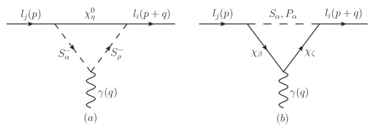
Figure 1: Feynman diagrams for the LFV process $l_{j}^{-}\rightarrow l_{i}^{-}\gamma$. (a) represents the contributions from neutral fermions $\chi_{\eta}^{0}$ and charged scalars $S_{\alpha,\rho}^{-}$ loops, while (b) represents the contributions from charged fermions $\chi_{\beta,\zeta}$ and neutral scalars $N_{\alpha}$ ($N=S,P$) loops.

The amplitude for $l_{j}^{-}\rightarrow l_{i}^{-}\gamma$ (including $\mu\rightarrow e\gamma$ and $\tau\rightarrow\mu\gamma$ ) is generally written as [18]

$$T=e{\epsilon^{\mu}}{\bar{u}_{i}}(p+q)\Big{[}q^{2}{\gamma_{\mu}}(A_{1}^{L}{P_{L}}+A_{1}^{R}{P_{R}})$$

$$\qquad+\>{m_{{l_{j}}}}i{\sigma_{\mu\nu}}{q^{\nu}}(A_{2}^{L}{P_{L}}+A_{2}^{R}{P_{R}})\Big{]}{u_{j}}(p)\>,$$ (25)

where $q$ is the injecting photon momentum, $p$ is the injecting lepton momentum, and $m_{{l_{j}}}$ is the mass of the $j$-th generation charged lepton, respectively. Furthermore, $\epsilon$ is the photon polarization vector, ${u_{i}}(p)$ (${v_{i}}(p)$ in the expressions below) is the wave function for lepton (antilepton), and $P_{L}=\frac{1}{2}{(1-{\gamma_{5}})}$, $P_{R}=\frac{1}{2}{(1+{\gamma_{5}})}$. Here, the Feynman diagrams contributing to the above amplitude are shown in Fig.1. And the coefficients can be written by

$$A_{a}^{L,R}=A_{a}^{(n)L,R}+A_{a}^{(c)L,R}\quad(a=1,2)\>,$$ (26)

where $A_{a}^{(n)L,R}$ denote the contributions from the virtual neutral fermion loops, and $A_{a}^{(c)L,R}$ stand for the contributions from the virtual charged fermion loops, respectively. After integrating the heavy freedoms out, we formulate those coefficients as follows

$$A_{1}^{(n)L}=\frac{1}{6{m_{W}^{2}}}C_{R}^{S_{\alpha}^{-}\chi_{\eta}^{\circ}{{\bar{\chi}}_{i}}}C_{L}^{S_{\alpha}^{-\ast}{\chi_{j}}\bar{\chi}_{\eta}^{\circ}}{I_{4}}({x_{\chi_{\eta}^{\circ}}},{x_{S_{\alpha}^{-}}})\;,$$

$$A_{2}^{(n)L}=\frac{{{m_{\chi_{\eta}^{\circ}}}}}{{{m_{{l_{j}}}}}{m_{W}^{2}}}C_{L}^{S_{\alpha}^{-}\chi_{\eta}^{\circ}{{\bar{\chi}}_{i}}}C_{L}^{S_{\alpha}^{-\ast}{\chi_{j}}\bar{\chi}_{\eta}^{\circ}}\Big{[}{I_{3}}({x_{\chi_{\eta}^{\circ}}},{x_{S_{\alpha}^{-}}})-{I_{1}}({x_{\chi_{\eta}^{\circ}}},{x_{S_{\alpha}^{-}}})\Big{]}\;,$$

$$A_{a}^{(n)R}=\left.{A_{a}^{(n)L}}\right|{{}_{L\leftrightarrow R}}\>,$$ (27)

where the concrete expressions for form factors $I_{k}\>(k=1,\ldots,4)$ can be found in E. Additionally, $x={m^{2}}/{m_{W}^{2}}$, $m$ is the mass for the corresponding particle and $m_{W}$ is the mass for the $W$-boson, respectively. In a similar way, the corrections from the Feynman diagrams with virtual charged fermions are

$$A_{1}^{(c)L}=\sum\limits_{N=S,P}\frac{1}{6{m_{W}^{2}}}C_{R}^{{N_{\alpha}}{\chi_{\beta}}{{\bar{\chi}}_{i}}}C_{L}^{{N_{\alpha}}{\chi_{j}}{{\bar{\chi}}_{\beta}}}\Big{[}{I_{1}}({x_{{\chi_{\beta}}}},{x_{{N_{\alpha}}}})-2{I_{2}}({x_{{\chi_{\beta}}}},{x_{{N_{\alpha}}}})$$

$$\qquad\qquad\qquad-{I_{4}}({x_{{\chi_{\beta}}}},{x_{{N_{\alpha}}}})\Big{]}\;,$$

$$A_{2}^{(c)L}=\sum\limits_{N=S,P}\frac{{{m_{{\chi_{{}^{\beta}}}}}}}{{{m_{{l_{j}}}}}{m_{W}^{2}}}C_{L}^{{N_{\alpha}}{\chi_{\beta}}{{\bar{\chi}}_{i}}}C_{L}^{{N_{\alpha}}{\chi_{j}}{{\bar{\chi}}_{\beta}}}\Big{[}{I_{1}}({x_{{\chi_{\beta}}}},{x_{{N_{\alpha}}}})-{I_{2}}({x_{{\chi_{\beta}}}},{x_{{N_{\alpha}}}})$$

$$\qquad\qquad\qquad-{I_{4}}({x_{{\chi_{\beta}}}},{x_{{N_{\alpha}}}})\Big{]}\;,$$

$$A_{a}^{(c)R}=\left.{A_{a}^{(c)L}}\right|{{}_{L\leftrightarrow R}}\>.$$ (28)

Using the amplitude presented in Eq.(25), we then obtain the decay width for $l_{j}^{-}\rightarrow l_{i}^{-}\gamma$ as [18]

$$\Gamma(l_{j}^{-}\to l_{i}^{-}\gamma)=\frac{{{e^{2}}}}{{16\pi}}m_{{l_{j}}}^{5}\Big{(}{\left|{A_{2}^{L}}\right|^{2}}+{\left|{A_{2}^{R}}\right|^{2}}\Big{)}\>.$$ (29)

And the branching ratio of $l_{j}^{-}\rightarrow l_{i}^{-}\gamma$ is

$${\rm{Br}}(l_{j}^{-}\to l_{i}^{-}\gamma)=\frac{\Gamma(l_{j}^{-}\to l_{i}^{-}\gamma)}{\Gamma_{l_{j}^{-}}}\>,$$ (30)

where $\Gamma_{l_{j}^{-}}$ denotes the total decay rate of the lepton $l_{j}^{-}$. In the numerical calculation, $\Gamma_{\mu}\approx 2.996\times 10^{-19}\>{\rm{GeV}}$ for the muon and $\Gamma_{\tau}\approx 2.265\times 10^{-12}\>{\rm{GeV}}$ for the tauon.

3.2 Rare decay $l_{j}^{-}\rightarrow l_{i}^{-}l_{i}^{-}l_{i}^{+}$

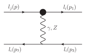
Figure 2: Penguin-type diagrams for the LFV process $l_{j}^{-}\rightarrow l_{i}^{-}l_{i}^{-}l_{i}^{+}$ in which a photon $\gamma$ and $Z$-boson are exchanged. The blob indicates an $l_{j}^{-}-l_{i}^{-}-\gamma$ vertex such as Fig.1 or $l_{j}^{-}-l_{i}^{-}-Z$ vertex where the $Z$-boson is external.

For the rare LFV processes $l_{j}^{-}\rightarrow l_{i}^{-}l_{i}^{-}l_{i}^{+}$ (including $\mu\rightarrow 3e$), the corresponding effective Hamilton originates from penguin-type diagrams and from box-type diagrams. The $\gamma$-penguin contribution can be computed using Eq.(25), with the result

$$T_{\gamma-{\rm{p}}}={\bar{u}_{i}}({p_{1}})\Big{[}{q^{2}}{\gamma_{\mu}}(A_{1}^{L}{P_{L}}+A_{1}^{R}{P_{R}})+{m_{l_{j}}}i{\sigma_{\mu\nu}}{q^{\nu}}(A_{2}^{L}{P_{L}}+A_{2}^{R}{P_{R}})\Big{]}{u_{j}}(p)$$

$$\qquad\quad\;\;\times\>\frac{{{e^{2}}}}{{{q^{2}}}}{\bar{u}_{i}}({p_{2}}){\gamma^{\mu}}{v_{i}}({p_{3}})-({p_{1}}\leftrightarrow{p_{2}})\>.$$ (31)

Similarly, the contribution from $Z$-penguin diagrams which are depicted by Fig.2 is

$$T_{Z-{\rm{p}}}=\frac{{{e^{2}}}}{{m_{Z}^{2}}}{\bar{u}_{i}}({p_{1}}){\gamma_{\mu}}({F_{L}}{P_{L}}+{F_{R}}{P_{R}}){u_{j}}(p){\bar{u}_{i}}({p_{2}}){\gamma^{\mu}}\Big{(}C_{L}^{Z{\chi_{2+i}}{\bar{\chi}_{2+i}}}{P_{L}}\qquad$$

$$\qquad\quad\;\;+\>C_{R}^{Z{\chi_{2+i}}{\bar{\chi}_{2+i}}}{P_{R}}\Big{)}{v_{i}}({p_{3}})-({p_{1}}\leftrightarrow{p_{2}})\>,$$ (32)

where $m_{Z}$ is the mass for the $Z$-boson and

$${F_{L,R}}=F_{L,R}^{(n)}+F_{L,R}^{(c)}\>.$$ (33)

The contributions to the effective couplings $F_{L,R}^{(n)}$ and $F_{L,R}^{(c)}$ are

$$F_{L}^{(n)}=\sum\limits_{N=S,P}\Big{[}\frac{{m_{{\chi_{\zeta}}}}{m_{{\chi_{\beta}}}}}{{e^{2}}{m_{W}^{2}}}C_{R}^{{N_{\alpha}}{\chi_{\zeta}}{{\bar{\chi}}_{i}}}C_{L}^{Z{\chi_{\beta}}{{\bar{\chi}}_{\zeta}}}C_{L}^{{N_{\alpha}}{\chi_{j}}{{\bar{\chi}}_{\beta}}}{G_{1}}({x_{{N_{\alpha}}}},{x_{{\chi_{\zeta}}}},{x_{{\chi_{\beta}}}})$$

$$\qquad\;\quad-\>\frac{1}{2{e^{2}}}C_{R}^{{N_{\alpha}}{\chi_{\zeta}}{{\bar{\chi}}_{i}}}C_{R}^{Z{\chi_{\beta}}{{\bar{\chi}}_{\zeta}}}C_{L}^{{N_{\alpha}}{\chi_{j}}{{\bar{\chi}}_{\beta}}}{G_{2}}({x_{{N_{\alpha}}}},{x_{{\chi_{\zeta}}}},{x_{{\chi_{\beta}}}})\Big{]}\>,$$

$$F_{L}^{(c)}=\,\frac{1}{2{e^{2}}}C_{R}^{S_{\rho}^{-}\chi_{\eta}^{0}{{\bar{\chi}}_{i}}}C_{R}^{ZS_{\alpha}^{-}S_{\rho}^{-\ast}}C_{L}^{S_{\alpha}^{-\ast}{\chi_{j}}\bar{\chi}_{\eta}^{0}}{G_{2}}({x_{\chi_{\eta}^{0}}},{x_{S_{\alpha}^{-}}},{x_{S_{\rho}^{-}}})\>,$$

$$F_{R}^{(n,c)}=\left.{F_{L}^{(n,c)}}\right|{{}_{L\leftrightarrow R}}\>.$$ (34)

Here, the concrete expressions for $G_{k}$ are given in E.

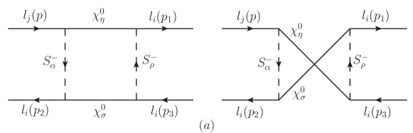
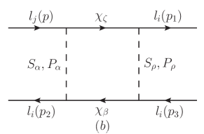
Figure 3: Box-type diagrams for the LFV process $l_{j}^{-}\rightarrow l_{i}^{-}l_{i}^{-}l_{i}^{+}$. (a) represents the contributions from neutral fermions $\chi_{\eta,\sigma}^{0}$ and charged scalars $S_{\alpha,\rho}^{-}$ loops, and (b) represents the contributions from charged fermions $\chi_{\beta,\zeta}$ and neutral scalars $N_{\alpha,\rho}$ ($N=S,P$) loops.

Furthermore, the effective Hamilton from the box-type diagrams which are drawn in Fig.3 can be written as

$$T_{box}=\Big{\{}B_{1}^{L}{e^{2}}{\bar{u}_{i}}({p_{1}}){\gamma_{\mu}}{P_{L}}{u_{j}}(p){\bar{u}_{i}}(p_{2}){\gamma^{\mu}}{P_{L}}{v_{i}}({p_{3}})+(L\leftrightarrow R)\Big{\}}$$

$$\quad+\>\Big{\{}B_{2}^{L}{e^{2}}\Big{[}{\bar{u}_{i}}(p_{1}){\gamma_{\mu}}{P_{L}}{u_{j}}(p){\bar{u}_{i}}(p_{2}){\gamma^{\mu}}{P_{R}}{v_{i}}({p_{3}})-(p_{1}\leftrightarrow{p_{2}})\Big{]}+{(L\leftrightarrow R)}\Big{\}}$$

$$\quad+\>\Big{\{}B_{3}^{L}{e^{2}}\Big{[}{\bar{u}_{i}}({p_{1}}){P_{L}}{u_{j}}(p){\bar{u}_{i}}({p_{2}}){P_{L}}{v_{i}}({p_{3}})-({p_{1}}\leftrightarrow{p_{2}})\Big{]}+(L\leftrightarrow R)\Big{\}}$$

$$\quad+\>\Big{\{}B_{4}^{L}{e^{2}}\Big{[}{\bar{u}_{i}}({p_{1}}){\sigma_{\mu\nu}}{P_{L}}{u_{j}}(p){\bar{u}_{i}}({p_{2}}){\sigma^{\mu\nu}}{P_{L}}{v_{i}}({p_{3}})-({p_{1}}\leftrightarrow{p_{2}})\Big{]}+\>(L\leftrightarrow R)\Big{\}}\>$$

with

$$B_{a}^{L,R}=B_{a}^{(n)L,R}+B_{a}^{(c)L,R}\quad(a=1,\ldots,4)\>.$$ (36)

The effective couplings $B_{a}^{(n)L,R}$ originate from those box diagrams with virtual neutral fermion contributions:

$$B_{1}^{(n)L}=\frac{{m_{\chi_{\eta}^{0}}}{m_{\chi_{\sigma}^{0}}}}{{e^{2}}{m_{W}^{4}}}{G_{3}}({x_{\chi_{\eta}^{0}}},{x_{\chi_{\sigma}^{0}}},{x_{S_{\alpha}^{-}}},{x_{S_{\rho}^{-}}})C_{L}^{S_{\rho}^{-}\chi_{\eta}^{0}{{\bar{\chi}}_{i}}}C_{L}^{S_{\alpha}^{-\ast}{\chi_{j}}\bar{\chi}_{\eta}^{0}}C_{R}^{S_{\rho}^{-}\chi_{\sigma}^{0}{{\bar{\chi}}_{i}}}C_{R}^{S_{\alpha}^{-\ast}{\chi_{i}}\bar{\chi}_{\sigma}^{0}}$$

$$\qquad\;\quad+\>\frac{1}{2{e^{2}}{m_{W}^{2}}}{G_{4}}({x_{\chi_{\eta}^{0}}},{x_{\chi_{\sigma}^{0}}},{x_{S_{\alpha}^{-}}},{x_{S_{\rho}^{-}}})\Big{[}C_{R}^{S_{\rho}^{-}\chi_{\eta}^{0}{{\bar{\chi}}_{i}}}C_{L}^{S_{\alpha}^{-\ast}{\chi_{j}}\bar{\chi}_{\eta}^{0}}C_{R}^{S_{\alpha}^{-}\chi_{\sigma}^{0}{{\bar{\chi}}_{i}}}C_{L}^{S_{\rho}^{-\ast}{\chi_{i}}\bar{\chi}_{\sigma}^{0}}$$

$$\qquad\;\quad+\>C_{L}^{S_{\rho}^{-}\chi_{\eta}^{0}{{\bar{\chi}}_{i}}}C_{R}^{S_{\alpha}^{-\ast}{\chi_{j}}\bar{\chi}_{\eta}^{0}}C_{R}^{S_{\rho}^{-}\chi_{\sigma}^{0}{{\bar{\chi}}_{i}}}C_{L}^{S_{\alpha}^{-\ast}{\chi_{i}}\bar{\chi}_{\sigma}^{0}}\Big{]},$$

$$B_{2}^{(n)L}=-\frac{{m_{\chi_{\eta}^{0}}}{m_{\chi_{\sigma}^{0}}}}{2{e^{2}}{m_{W}^{4}}}{G_{3}}({x_{\chi_{\eta}^{0}}},{x_{\chi_{\sigma}^{0}}},{x_{S_{\alpha}^{-}}},{x_{S_{\rho}^{-}}})C_{R}^{S_{\rho}^{-}\chi_{\eta}^{0}{{\bar{\chi}}_{i}}}C_{R}^{S_{\alpha}^{-\ast}{\chi_{j}}\bar{\chi}_{\eta}^{0}}C_{L}^{S_{\alpha}^{-}\chi_{\sigma}^{0}{{\bar{\chi}}_{i}}}C_{L}^{S_{\rho}^{-\ast}{\chi_{i}}\bar{\chi}_{\sigma}^{0}}$$

$$\qquad\;\quad+\>\frac{1}{4{e^{2}}{m_{W}^{2}}}{G_{4}}({x_{\chi_{\eta}^{0}}},{x_{\chi_{\sigma}^{0}}},{x_{S_{\alpha}^{-}}},{x_{S_{\rho}^{-}}})\Big{[}C_{R}^{S_{\rho}^{-}\chi_{\eta}^{0}{{\bar{\chi}}_{i}}}C_{L}^{S_{\alpha}^{-\ast}{\chi_{j}}\bar{\chi}_{\eta}^{0}}C_{L}^{S_{\alpha}^{-}\chi_{\sigma}^{0}{{\bar{\chi}}_{i}}}C_{R}^{S_{\rho}^{-\ast}{\chi_{i}}\bar{\chi}_{\sigma}^{0}}$$

$$\qquad\;\quad+\>C_{R}^{S_{\rho}^{-}\chi_{\eta}^{0}{{\bar{\chi}}_{i}}}C_{L}^{S_{\alpha}^{-\ast}{\chi_{j}}\bar{\chi}_{\eta}^{0}}C_{R}^{S_{\rho}^{-}\chi_{\sigma}^{0}{{\bar{\chi}}_{i}}}C_{L}^{S_{\alpha}^{-\ast}{\chi_{i}}\bar{\chi}_{\sigma}^{0}}\Big{]},$$

$$B_{3}^{(n)L}=\frac{{m_{\chi_{\eta}^{0}}}{m_{\chi_{\sigma}^{0}}}}{{e^{2}}{m_{W}^{4}}}{G_{3}}({x_{\chi_{\eta}^{0}}},{x_{\chi_{\sigma}^{0}}},{x_{S_{\alpha}^{-}}},{x_{S_{\rho}^{-}}})\Big{[}C_{L}^{S_{\rho}^{-}\chi_{\eta}^{0}{{\bar{\chi}}_{i}}}C_{L}^{S_{\alpha}^{-\ast}{\chi_{j}}\bar{\chi}_{\eta}^{0}}C_{L}^{S_{\alpha}^{-}\chi_{\sigma}^{0}{{\bar{\chi}}_{i}}}C_{L}^{S_{\rho}^{-\ast}{\chi_{i}}\bar{\chi}_{\sigma}^{0}}$$

$$\qquad\;\quad-\>\frac{1}{2}\>C_{L}^{S_{\rho}^{-}\chi_{\eta}^{0}{{\bar{\chi}}_{i}}}C_{L}^{S_{\alpha}^{-\ast}{\chi_{j}}\bar{\chi}_{\eta}^{0}}C_{L}^{S_{\rho}^{-}\chi_{\sigma}^{0}{{\bar{\chi}}_{i}}}C_{L}^{S_{\alpha}^{-\ast}{\chi_{i}}\bar{\chi}_{\sigma}^{0}}\Big{]},$$

$$B_{4}^{(n)L}=\frac{{m_{\chi_{\eta}^{0}}}{m_{\chi_{\sigma}^{0}}}}{8{e^{2}}{m_{W}^{4}}}{G_{3}}({x_{\chi_{\eta}^{0}}},{x_{\chi_{\sigma}^{0}}},{x_{S_{\alpha}^{-}}},{x_{S_{\rho}^{-}}})C_{L}^{S_{\rho}^{-}\chi_{\eta}^{0}{{\bar{\chi}}_{i}}}C_{L}^{S_{\alpha}^{-\ast}{\chi_{j}}\bar{\chi}_{\eta}^{0}}C_{L}^{S_{\rho}^{-}\chi_{\sigma}^{0}{{\bar{\chi}}_{i}}}C_{L}^{S_{\alpha}^{-\ast}{\chi_{i}}\bar{\chi}_{\sigma}^{0}},$$

$$B_{a}^{(n)R}=\left.{B_{a}^{(n)L}}\right|{{}_{L\leftrightarrow R}}\>.$$ (37)

Correspondingly, the effective couplings from the box diagrams with virtual charged fermion contributions $B_{a}^{(c)L,R}$ are

$$B_{1}^{(c)L}=\sum\limits_{N=S,P}\frac{1}{2{e^{2}}{m_{W}^{2}}}{G_{4}}({x_{{\chi_{\zeta}}}},{x_{{\chi_{\beta}}}},{x_{{N_{\alpha}}}},{x_{{N_{\rho}}}})C_{R}^{{N_{\rho}}{\chi_{\zeta}}{{\bar{\chi}}_{i}}}C_{L}^{{N_{\alpha}}{\chi_{j}}{{\bar{\chi}}_{\zeta}}}C_{R}^{{N_{\alpha}}{\chi_{\beta}}{{\bar{\chi}}_{i}}}C_{L}^{{N_{\rho}}{\chi_{i}}{{\bar{\chi}}_{\beta}}},$$

$$B_{2}^{(c)L}=\sum\limits_{N=S,P}\Big{[}\frac{1}{4{e^{2}}{m_{W}^{2}}}{G_{4}}({x_{{\chi_{\zeta}}}},{x_{{\chi_{\beta}}}},{x_{{N_{\alpha}}}},{x_{{N_{\rho}}}})C_{R}^{{N_{\rho}}{\chi_{\zeta}}{{\bar{\chi}}_{i}}}C_{L}^{{N_{\alpha}}{\chi_{j}}{{\bar{\chi}}_{\zeta}}}C_{L}^{{N_{\alpha}}{\chi_{\beta}}{{\bar{\chi}}_{i}}}C_{R}^{{N_{\rho}}{\chi_{i}}{{\bar{\chi}}_{\beta}}}$$

$$\qquad\;\;\quad-\frac{{m_{\chi_{\zeta}}}{m_{\chi_{\beta}}}}{2{e^{2}}{m_{W}^{4}}}{G_{3}}({x_{{\chi_{\zeta}}}},{x_{{\chi_{\beta}}}},{x_{{N_{\alpha}}}},{x_{{N_{\rho}}}})C_{R}^{{N_{\rho}}{\chi_{\zeta}}{{\bar{\chi}}_{i}}}C_{R}^{{N_{\alpha}}{\chi_{j}}{{\bar{\chi}}_{\zeta}}}C_{L}^{{N_{\alpha}}{\chi_{\beta}}{{\bar{\chi}}_{i}}}C_{L}^{{N_{\rho}}{\chi_{i}}{{\bar{\chi}}_{\beta}}}\Big{]},$$

$$B_{3}^{(c)L}=\sum\limits_{N=S,P}\frac{{m_{\chi_{\zeta}}}{m_{\chi_{\beta}}}}{{e^{2}}{m_{W}^{4}}}{{G_{3}}({x_{{\chi_{\zeta}}}},{x_{{\chi_{\beta}}}},{x_{{N_{\alpha}}}},{x_{{N_{\rho}}}})C_{L}^{{N_{\rho}}{\chi_{\zeta}}{{\bar{\chi}}_{i}}}C_{L}^{{N_{\alpha}}{\chi_{j}}{{\bar{\chi}}_{\zeta}}}C_{L}^{{N_{\alpha}}{\chi_{\beta}}{{\bar{\chi}}_{i}}}C_{L}^{{N_{\rho}}{\chi_{i}}{{\bar{\chi}}_{\beta}}}},$$

$$B_{4}^{(c)L}=0\>,$$

$$B_{a}^{(c)R}=\left.{B_{a}^{(c)L}}\right|{{}_{L\leftrightarrow R}}\>.$$ (38)

Using the expression for the above amplitude, we can calculate the decay width for $l_{j}^{-}\rightarrow l_{i}^{-}l_{i}^{-}l_{i}^{+}$ [18]:

$$\Gamma(l_{j}^{-}\to l_{i}^{-}l_{i}^{-}l_{i}^{+})=\frac{{{e^{4}}}}{{512{\pi^{3}}}}m_{{l_{j}}}^{5}\Big{\{}({\left|{A_{2}^{L}}\right|^{2}}+{\left|{A_{2}^{R}}\right|^{2}})(\frac{{16}}{3}\ln\frac{{{m_{{l_{j}}}}}}{{2{m_{{l_{i}}}}}}-\frac{{14}}{9})$$

$$\quad+\>({\left|{A_{1}^{L}}\right|^{2}}+{\left|{A_{1}^{R}}\right|^{2}})-2(A_{1}^{L}A_{2}^{R*}+A_{2}^{L}A_{1}^{R*}+\textrm{H.c.})+\frac{1}{6}({\left|{B_{1}^{L}}\right|^{2}}+{\left|{B_{1}^{R}}\right|^{2}})$$

$$\quad+\>\frac{1}{3}({\left|{B_{2}^{L}}\right|^{2}}+{\left|{B_{2}^{R}}\right|^{2}})+\frac{1}{{24}}({\left|{B_{3}^{L}}\right|^{2}}+{\left|{B_{3}^{R}}\right|^{2}})+6({\left|{B_{4}^{L}}\right|^{2}}+{\left|{B_{4}^{R}}\right|^{2}})$$

$$\quad-\>\frac{1}{2}(B_{3}^{L}B_{4}^{L*}+B_{3}^{R}A_{4}^{R*}+\textrm{H.c.})+\frac{1}{3}(A_{1}^{L}B_{1}^{L*}+A_{1}^{R}B_{1}^{R*}+A_{1}^{L}B_{2}^{L*}$$

$$\quad+\>A_{1}^{R}B_{2}^{R*}+\textrm{H.c.})-\frac{2}{3}(A_{2}^{R}B_{1}^{L*}+A_{2}^{L}B_{1}^{R*}+A_{2}^{L}B_{2}^{R*}+A_{2}^{R}B_{2}^{L*}+\textrm{H.c.})$$

$$\quad+\>\frac{1}{3}\Big{[}2({\left|{{F_{LL}}}\right|^{2}}+{\left|{{F_{RR}}}\right|^{2}})+({\left|{{F_{LR}}}\right|^{2}}+{\left|{{F_{RL}}}\right|^{2}})+(B_{1}^{L}F_{LL}^{*}+B_{1}^{R}F_{RR}^{*}$$

$$\quad+\>B_{2}^{L}F_{LR}^{*}+B_{2}^{R}F_{RL}^{*}+\textrm{H.c.})+2(A_{1}^{L}F_{LL}^{*}+A_{1}^{R}F_{RR}^{*}+\textrm{H.c.})$$

$$\quad+\>(A_{1}^{L}F_{LR}^{*}+A_{1}^{R}F_{RL}^{*}+\textrm{H.c.})-4(A_{2}^{R}F_{LL}^{*}+A_{2}^{L}F_{RR}^{*}+\textrm{H.c.})$$

$$\quad-\>2(A_{2}^{L}F_{RL}^{*}+A_{2}^{R}F_{LR}^{*}+\textrm{H.c.})\Big{]}\Big{\}}\;$$ (39)

with

$${F_{LL}}=\frac{{{F_{L}}C_{L}^{Z{\chi_{2+i}}{\bar{\chi}_{2+i}}}}}{{m_{Z}^{2}}},\qquad{F_{RR}}={F_{LL}}\left|{{}_{L\leftrightarrow R}}\right.,\quad$$

$${F_{LR}}=\frac{{{F_{L}}C_{R}^{Z{\chi_{2+i}}{\bar{\chi}_{2+i}}}}}{{m_{Z}^{2}}},\qquad{F_{RL}}={F_{LR}}\left|{{}_{L\leftrightarrow R}}\right..\quad$$ (40)

And the branching ratio of $l_{j}^{-}\to l_{i}^{-}l_{i}^{-}l_{i}^{+}$ is

$${\rm{Br}}(l_{j}^{-}\to l_{i}^{-}l_{i}^{-}l_{i}^{+})=\frac{\Gamma(l_{j}^{-}\to l_{i}^{-}l_{i}^{-}l_{i}^{+})}{\Gamma_{l_{j}^{-}}}\>.$$ (41)

4 $(g-2)_{\mu}$ in the $\mu\nu$SSM

The anomalous magnetic dipole moment (MDM) of the muon can be actually be written as the operator

$$\mathcal{L}_{MDM}=\frac{e}{4m_{\mu}}a_{\mu}\bar{l}_{\mu}\sigma^{\alpha\beta}l_{\mu}F_{\alpha\beta}\>,$$ (42)

where $\sigma^{\alpha\beta}=\frac{i}{2}[\gamma^{\alpha},\gamma^{\beta}]$, $F_{\alpha\beta}$ is the electromagnetic field strength, $l_{\mu}$ denotes the muon which is on-shell, $m_{\mu}$ is the muon mass and $a_{\mu}=\frac{1}{2}(g-2)_{\mu}$. Adopting the effective Lagrangian approach, we can get [19]

$$a_{\mu}=\frac{4Q_{f}m_{\mu}^{2}}{{(4\pi)}^{2}}\Re{(C_{2}^{R}+C_{2}^{L\ast}+C_{6}^{R})}\>,$$ (43)

where $Q_{f}=-1$, $\Re(\cdots)$ represents the operation to take the real part of a complex number and $C_{2,6}^{L,R}$ denote the Wilson coefficients of the corresponding operators $O_{2,6}^{L,R}$

$$O_{2}^{L,R}=\frac{eQ_{f}}{{(4\pi)}^{2}}\overline{(i\mathcal{D}_{\alpha}l_{\mu})}\gamma^{\alpha}F\cdot\sigma P_{L,R}l_{\mu}\>,$$

$$O_{6}^{L,R}=\frac{eQ_{f}m_{\mu}}{{(4\pi)}^{2}}\overline{l}_{\mu}F\cdot\sigma P_{L,R}l_{\mu}\>.$$ (44)

In the $\mu\nu$SSM, the SUSY corrections can be written as

$$C_{2,6}^{L,R}=C_{2,6}^{{L,R}(n)}+C_{2,6}^{{L,R}(c)}\>.$$ (45)

The effective couplings $C_{2,6}^{{L,R}(n)}$ represent the contributions from the triangle diagrams with virtual neutralinos

$$C_{2}^{R(n)}=\frac{{(4\pi)}^{2}}{Q_{f}{m_{W}^{2}}}C_{L}^{S_{\alpha}^{-}\chi_{\eta}^{\circ}{{\bar{\chi}}_{4}}}C_{R}^{S_{\alpha}^{-\ast}{\chi_{4}}\bar{\chi}_{\eta}^{\circ}}\Big{[}-{I_{3}}{\rm{(}}{x_{\chi_{\eta}^{\circ}}},{x_{S_{\alpha}^{-}}})+{I_{4}}({x_{\chi_{\eta}^{\circ}}},{x_{S_{\alpha}^{-}}})\Big{]}\>,$$

$$C_{6}^{R(n)}=\frac{{(4\pi)}^{2}{m_{\chi_{\eta}^{\circ}}}}{Q_{f}{m_{W}^{2}}{m_{\mu}}}C_{R}^{S_{\alpha}^{-}\chi_{\eta}^{\circ}{{\bar{\chi}}_{4}}}C_{R}^{S_{\alpha}^{-\ast}{\chi_{4}}\bar{\chi}_{\eta}^{\circ}}\Big{[}-2{I_{1}}({x_{\chi_{\eta}^{\circ}}},{x_{S_{\alpha}^{-}}})+2{I_{3}}({x_{\chi_{\eta}^{\circ}}},{x_{S_{\alpha}^{-}}})\Big{]}\>,$$

$$C_{2,6}^{L(n)}=C_{2,6}^{R(n)}\mid_{L\leftrightarrow R}\>.$$ (46)

Similarly, the contributions $C_{2,6}^{{L,R}(c)}$ originating from triangle diagrams with virtual charginos are

$$C_{2}^{R(c)}=\sum\limits_{N=S,P}\frac{{(4\pi)}^{2}}{Q_{f}{m_{W}^{2}}}C_{R}^{{N_{\alpha}}{\chi_{\beta}}{{\bar{\chi}}_{4}}}C_{L}^{{N_{\alpha}}{\chi_{4}}{{\bar{\chi}}_{\beta}}}\Big{[}-{I_{1}}({x_{{\chi_{\beta}}}},{x_{{N_{\alpha}}}})+2{I_{3}}({x_{{\chi_{\beta}}}},{x_{{N_{\alpha}}}})$$

$$\qquad\qquad\qquad-{I_{4}}({x_{{\chi_{\beta}}}},{x_{{N_{\alpha}}}})\Big{]}\>,$$

$$C_{6}^{R(c)}=\sum\limits_{N=S,P}\frac{{(4\pi)}^{2}{m_{{\chi_{{}^{\beta}}}}}}{Q_{f}{m_{W}^{2}}{m_{\mu}}}C_{R}^{{N_{\alpha}}{\chi_{\beta}}{{\bar{\chi}}_{4}}}C_{R}^{{N_{\alpha}}{\chi_{4}}{{\bar{\chi}}_{\beta}}}\Big{[}2{I_{1}}({x_{{\chi_{\beta}}}},{x_{{N_{\alpha}}}})-2{I_{2}}({x_{{\chi_{\beta}}}},{x_{{N_{\alpha}}}})$$

$$\qquad\qquad\qquad-2{I_{3}}({x_{{\chi_{\beta}}}},{x_{{N_{\alpha}}}})\Big{]}\>,$$

$$C_{2,6}^{L(c)}=C_{2,6}^{R(c)}\mid_{L\leftrightarrow R}\,.$$ (47)

5 The numerical results

5.1 The parameter space

It is well known that there are many free parameters in various SUSY extensions of the SM. In order to obtain a more transparent numerical results, we take some assumptions on parameter space of the $\mu\nu{\rm SSM}$ before we perform the numerical analysis.

In lepton sector, we adopt the minimal flavor violation (MFV) assumptions

$${\kappa_{ijk}}=\kappa\textrm{ and }{({A_{\kappa}}\kappa)_{ijk}}={A_{\kappa}}\kappa,\,\textrm{if }i=j=k,\,\textrm{and zero otherwise},$$

$$m_{{{\tilde{L}}_{ij}}}^{2}=m_{\tilde{L}_{i}}^{2}{\delta_{ij}},\>m_{\tilde{\nu}_{ij}^{c}}^{2}=m_{{{\tilde{\nu}_{i}}^{c}}}^{2}{\delta_{ij}},\>m_{\tilde{e}_{ij}^{c}}^{2}=m_{{{\tilde{e}}^{c}}}^{2}{\delta_{ij}},$$

$${Y_{{\nu_{ij}}}}={Y_{{\nu_{i}}}}{\delta_{ij}},\>{Y_{{e_{ij}}}}={Y_{{e_{i}}}}{\delta_{ij}},\>\lambda_{i}=\lambda,\>\upsilon_{\nu_{i}^{c}}=\upsilon_{\nu^{c}},$$

$$(A_{\nu}Y_{\nu})_{ij}={A_{\nu}}{Y_{{\nu_{i}}}}{\delta_{ij}},\>{({A_{e}}{Y_{e}})_{ij}}={A_{e}}{Y_{{e_{i}}}}{\delta_{ij}}\>,\>\textrm{and }{{\rm{(}}{A_{\lambda}}\lambda{\rm{)}}_{i}}={A_{\lambda}}\lambda,$$ (48)

where $i,\;j,\;k=1,\;2,\;3$.

The $3\times 3$ matrix $Y_{\nu}$ determines the Dirac masses for the neutrinos ${Y_{\nu}}{\upsilon_{u}}\sim{m_{D}}$, and the tiny neutrino masses are obtained through TeV scale seesaw mechanism $m_{\nu}\sim m_{D}m_{{}_{N}}^{-1}m_{D}^{T}$. This indicates that the nonzero VEVs of left-handed sneutrinos satisfy $\upsilon_{\nu_{i}}\ll\upsilon_{u,d}$, then

$$\tan\beta\simeq\frac{\upsilon_{u}}{\upsilon_{d}}\>.$$ (49)

Assuming that the charged lepton mass matrix in the flavor basic is in the diagonal form, we get

$${Y_{{e_{i}}}}=\frac{{{m_{{l_{i}}}}}}{{{\upsilon_{d}}}},$$ (50)

where $m_{l_{i}}$ is the charged lepton $l_{i}$ mass, and we parameterize the unitary matrix which diagonalizes the effective light neutrino mass matrix $m_{eff}$ (can be found in C) as [20]

$${U_{\nu}}= \left({\begin{array}[]{*{20}{c}}{{c_{12}}{c_{13}}}&{{s_{12}}{c_{13}}}&{{s_{13}}{e^{-i\delta}}}\\ {-{s_{12}}{c_{23}}-{c_{12}}{s_{23}}{s_{13}}{e^{i\delta}}}&{{c_{12}}{c_{23}}-{s_{12}}{s_{23}}{s_{13}}{e^{i\delta}}}&{{s_{23}}{c_{13}}}\\ {{s_{12}}{s_{23}}-{c_{12}}{c_{23}}{s_{13}}{e^{i\delta}}}&{-{c_{12}}{s_{23}}-{s_{12}}{c_{23}}{s_{13}}{e^{i\delta}}}&{{c_{23}}{c_{13}}}\\ \end{array}}\right)$$ (55)

$$\>\times\>diag(1,{e^{i\frac{{{\alpha_{21}}}}{2}}},{e^{i\frac{{{\alpha_{31}}}}{2}}})\>,$$

where ${c_{ij}}=\cos{\theta_{ij}}$, ${s_{ij}}=\sin{\theta_{ij}}$, the angles ${\theta_{ij}}=\left[\>{0,\pi/2}\>\right]$, $\delta=\left[\>{0,2\pi}\>\right]$ is the Dirac CP violation phase and $\alpha_{21}$, $\alpha_{31}$ are two Majorana CP violation phases. Here, we choose $\delta=\alpha_{21}=\alpha_{31}=0$. $U_{\nu}$ diagonalizes $m_{eff}$ in the following way:

$$U_{\nu}^{T}m_{eff}^{T}{m_{eff}}{U_{\nu}}=diag({m_{\nu_{1}}^{2}},{m_{\nu_{2}}^{2}},{m_{\nu_{3}}^{2}})\>,$$ (56)

where the neutrino mass $m_{\nu_{i}}$ connected with experimental measurements through

$${m_{\nu_{2}}^{2}-m_{\nu_{1}}^{2}}={\Delta m_{21}^{2}},\qquad{m_{\nu_{3}}^{2}-m_{\nu_{2}}^{2}}={\Delta m_{32}^{2}}.$$ (57)

The combination of Eq.(55), Eq.(56), Eq.(57) with neutrino oscillation experimental data gives some strong constraints on relevant parameter space of the $\mu\nu$SSM.

At the EW scale, the soft masses $m_{\tilde{H}_{d}}^{2}$, $m_{\tilde{H}_{u}}^{2}$, $m_{\tilde{L}_{i}}^{2}$ and $m_{\tilde{\nu}_{i}^{c}}^{2}$ are derived from the minimization conditions of the tree-level neutral scalar potential, which are given in A. Implying the approximate GUT relation $M_{1}=\frac{\alpha_{1}^{2}}{\alpha_{2}^{2}}M_{2}\approx 0.5M_{2}$, the free parameters affect our analysis are

$$\lambda,\>\kappa,\>\tan\beta,\>{A_{\lambda,\kappa,\nu,e}},\>m_{{{\tilde{e}}^{c}}},\>{\upsilon_{\nu^{c}}},\>M_{2}\;.$$ (58)

To obtain the Yukawa couplings $Y_{\nu_{i}}$ and $\upsilon_{\nu_{i}}$ from Eq.(56), we assume the neutrinos masses satisfying ${m_{\nu_{1}}}{\rm{<}}{m_{\nu_{2}}}{\rm{<}}{m_{\nu_{3}}}$, and choose $m_{\nu_{2}}=10^{-2}\>{\rm{eV}}$ as input in our numerical analysis. Then we can get $m_{\nu_{1,3}}$ from the experimental data on the differences of neutrino mass squared. For $U_{\nu}$, the values of $\theta_{ij}$ are obtained from the experimental data in Eq.(1). And the effective light neutrino mass matrix $m_{eff}$ can approximate as [16]

$${m_{ef{f_{ij}}}}\approx\frac{{2A{\upsilon_{\nu^{c}}}}}{{3\Delta}}{b_{i}}{b_{j}}+\frac{{1-3{\delta_{ij}}}}{{6\kappa{\upsilon_{\nu^{c}}}}}{a_{i}}{a_{j}}\>,$$ (59)

where

$$\Delta={\lambda^{2}}{(\upsilon_{d}^{2}+\upsilon_{u}^{2})}^{2}+4\lambda\kappa{\upsilon_{\nu^{c}}^{2}}{\upsilon_{d}}{\upsilon_{u}}-12{\lambda^{2}}{\upsilon_{\nu^{c}}}AB\>,$$

$$A=\kappa{\upsilon_{\nu^{c}}^{2}}+\lambda{\upsilon_{d}}{\upsilon_{u}}\>,$$

$$\frac{1}{B}=\frac{e^{2}}{c_{{}_{W}}^{2}{M_{1}}}+\frac{e^{2}}{s_{{}_{W}}^{2}{M_{2}}}\>,$$

$${a_{i}}={Y_{{\nu_{i}}}}{\upsilon_{u}}\>,\quad{b_{i}}={Y_{{\nu_{i}}}}{\upsilon_{d}}+3\lambda\upsilon_{\nu_{i}}\>.$$ (60)

Then, we can numerically derive $Y_{\nu_{i}}\sim\mathcal{O}(10^{-7})$ and $\upsilon_{\nu_{i}}\sim\mathcal{O}(10^{-4}{\rm{GeV}})$ from Eq.(56).

5.2 Branching ratio of LFV processes

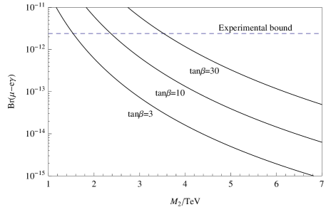
Figure 4: Branching ratio for the process $\mu\rightarrow e\gamma$ varies with $M_{2}$ for $\tan\beta=3,\;10,\;30$, respectively.

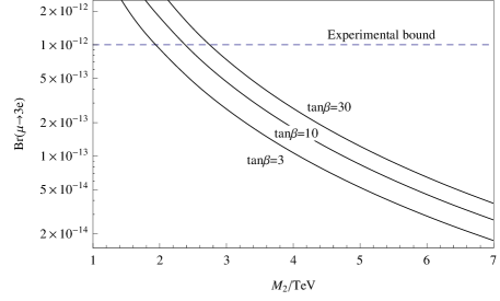
Figure 5: Branching ratio for the process $\mu\rightarrow 3e$ varies with $M_{2}$ for $\tan\beta=3,\;10,\;30$, respectively.

Considering the research of the $\mu\nu{\rm SSM}$ [4], we choose the relevant parameters as $\lambda=0.1$, $\kappa=0.01$, $m_{{{\tilde{e}}^{c}}}=A_{e}=A_{\lambda}=1\>{\rm{TeV}}$, $A_{\nu}=A_{\kappa}=-1\>{\rm{TeV}}$ and $\upsilon_{\nu^{c}}=800\>{\rm{GeV}}$ in next numerical analysis for convenience. With those assumptions on parameter space, we present the branching ratio of $\mu\rightarrow e\gamma$ versus $M_{2}$ in Fig.4. As $M_{2}\leq 2\>{\rm{TeV}}$, the theoretical evaluations exceed the upper experimental bound easily. The fact implies that experimental data do not favor small $M_{2}$. Along with increasing of $M_{2}$, theoretical evaluation on the branching ratio of $\mu\rightarrow e\gamma$ decreases steeply. As $M_{2}=3\>{\rm{TeV}}$ and $\tan\beta=10$, theoretical evaluation on the branching ratio of $\mu\rightarrow e\gamma$ is about $5\times 10^{-13}$ which can be detected in near future. In the future, the expected sensitivity for ${\rm{Br}}(\mu\rightarrow e\gamma)$ would be of order $10^{-13}$ [21]. Differing from LFV processes which are researched in the BRpV model [22], the large VEVs of right-handed sneutrinos in the $\mu\nu$SSM induce new sources for lepton-flavor violation. So, here the branching ratio of $\mu\rightarrow e\gamma$ can easily reach the upper experimental bound $2.4\times 10^{-12}$ [13].

We also investigate the $\mu\rightarrow 3e$ processes in detail. And the branching ratio of $\mu\rightarrow 3e$ is also decreases with increasing of $M_{2}$, and raises with increasing of $\tan\beta$, which is presented in the Fig.5. By Introducing the right-handed sneutrinos which the VEVs are nonzero to the $\mu\nu$SSM, the branching ratio of $\mu\rightarrow 3e$ can also easily reach the upper experimental bound $10^{-12}$ [13]. We can see that the experimental bounds of the branching ratio of $\mu\rightarrow 3e$ and $\mu\rightarrow e\gamma$ give very strong constraints on the $\mu\nu{\rm SSM}$.

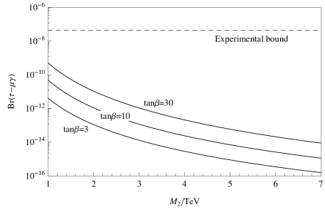
Figure 6: Branching ratio for the process $\tau\rightarrow\mu\gamma$ varies with $M_{2}$ for $\tan\beta=3,\;10,\;30$, respectively.

In Fig.6, we show the branching ratio for $\tau\rightarrow\mu\gamma$ versus $M_{2}$ as $\tan\beta=3,\;10,\;30$. Similar to the case of $\mu\rightarrow e\gamma$, the evaluation on the branching ratio for $\tau\rightarrow\mu\gamma$ decreases with increasing of $M_{2}$, and is enhanced by large $\tan\beta$. As $M_{2}=3\>{\rm TeV}$ and $\tan\beta=10$, ${\rm{Br}}(\tau\rightarrow\mu\gamma)\approx 10^{-13}$ is four orders below the expected sensitivity $10^{-9}$ [23].

5.3 Muon anomalous magnetic dipole moment

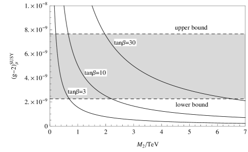
Figure 7: The SUSY contribution to the anomalous magnetic dipole moment of the muon varies with $M_{2}$ for $\tan\beta=3,\;10,\;30$, respectively. The gray area denotes the $\Delta a_{\mu}$ at $1.8$ standard deviation.

Finally, we analyze the anomalous magnetic dipole moment of the muon in the $\mu\nu$SSM. Rescaled the final result of the E821 Collaboration at BNL [24] using $\mu/p$ magnetic moment ratio of $3.183345137(85)$ from ref.[25], the PDG Collaboration [13] gives the world average of muon anomalous magnetic dipole moment

$$a_{\mu}^{{\rm{exp}}}=\frac{1}{2}(g_{\mu}-2)=11659208.9(5.4)(3.3)\times 10^{-10}\>,$$ (61)

where the statistical and systematic uncertainties are given, respectively. And the Standard Model (SM) prediction [13] is

$$a_{\mu}^{{\rm{SM}}}=11659184.1(4.8)\times 10^{-10}\>.$$ (62)

So, the difference between experiment and the SM prediction

$$\Delta a_{\mu}=a_{\mu}^{{\rm{exp}}}-a_{\mu}^{{\rm{SM}}}=24.8(8.7)(4.8)\times 10^{-10}\>,$$ (63)

represents an interesting but not yet conclusive discrepancy of $1.8$ standard deviation. An alternate interpretation is that $\Delta a_{\mu}$ may be a new physics signal with supersymmetric particle loops as the leading candidate explanation. If treated the supersymmetry as the leading explanation, parameter space of the $\mu\nu$SSM should be constrained by the experimental data on $\Delta a_{\mu}$.

The SUSY contribution to the muon anomalous magnetic dipole moment in the $\mu\nu$SSM is shown in Fig.7. The result shows that when $\tan\beta=3$, $\Delta a_{\mu}$ constrains $M_{2}<1\>{\rm{TeV}}$, which is opposite to what the upper experimental bound of $\rm{Br}(\mu\rightarrow e\gamma)$ constrains. The fact implies that experimental data do not favor small $\tan\beta$ in the $\mu\nu$SSM with the MFV assumptions (48). When $\tan\beta=30$, $\Delta a_{\mu}$ constrains $2\>{\rm{TeV}}\leq M_{2}<7\>{\rm{TeV}}$, compared with that the upper experimental bound of $\rm{Br}(\mu\rightarrow e\gamma)$ constrains $M_{2}\geq 3.5\>{\rm{TeV}}$, the $M_{2}$ has more consistent interval. So, under the MFV assumptions, the $\mu\nu$SSM favors large $\tan\beta$ and $M_{2}$ for consistent with experimental data.

6 Conclusions

Besides the superfields of the MSSM, the $\mu\nu$SSM introduces three exotic right-handed sneutrinos $\hat{\nu}_{i}^{c}$ to solve the $\mu$ problem of the MSSM. And exotic right-handed sneutrinos which the vacuum expectation values are nonzero induce new sources for lepton-flavor violation. In addition, from the scalars for the $\mu\nu$SSM we strictly separate the Goldstone bosons, which disappear in the physical gauge.

Considering the updated experimental data on neutrino oscillations, we analyze various LFV processes and $(g-2)_{\mu}$ in the $\mu\nu$SSM. Numerical results indicate that the new physics corrections dominate the evaluation on the branching ratios of LFV processes in some parameter space of the $\mu\nu$SSM. And the theoretical predictions on the branching ratios of LFV processes $\mu\rightarrow e\gamma$ and $\mu\rightarrow 3e$ for large $\tan\beta$ can easily reach the present experimental upper bounds and be detected in near future. Additionally, the present experimental observations on $(g-2)_{\mu}$ also give very strong constraint on the model. Under the MFV assumptions (48), the $\mu\nu$SSM favors large $\tan\beta$ and $M_{2}$ for consistent with experimental data. Certainly, a neutral Higgs with mass $m_{h_{0}}\sim 124-126\;{\rm GeV}$ reported by ATLAS [26] and CMS [27] also contributes a strict constraint on relevant parameter space, we will discuss this problem elsewhere.

Appendix A Minimization of the potential

First, the eight minimization conditions of the tree-level neutral scalar potential are given below:

$$m_{{H_{d}}}^{2}\upsilon_{d}+\frac{G^{2}}{4}(\upsilon_{d}^{2}-\upsilon_{u}^{2}+\upsilon_{\nu_{i}}\upsilon_{\nu_{i}})\upsilon_{d}-(A_{\lambda}\lambda)_{i}{\upsilon_{u}}\upsilon_{\nu_{i}^{c}}-{\lambda_{j}}{\kappa_{ijk}}{\upsilon_{u}}\upsilon_{\nu_{i}^{c}}\upsilon_{\nu_{k}^{c}}$$

$$\qquad+\>({\lambda_{i}}{\lambda_{j}}\upsilon_{\nu_{i}^{c}}\upsilon_{\nu_{j}^{c}}+{\lambda_{i}}{\lambda_{i}}\upsilon_{u}^{2}){\upsilon_{d}}-{Y_{{\nu_{ij}}}}\upsilon_{\nu_{i}}({\lambda_{k}}\upsilon_{\nu_{k}^{c}}\upsilon_{\nu_{j}^{c}}+{\lambda_{j}}\upsilon_{u}^{2})=0\>,$$ (64)

$$m_{{H_{u}}}^{2}{\upsilon_{u}}-\frac{{G^{2}}}{4}(\upsilon_{d}^{2}-\upsilon_{u}^{2}+\upsilon_{\nu_{i}}\upsilon_{\nu_{i}})\upsilon_{u}+{(A_{\nu}Y_{\nu})}_{ij}\upsilon_{\nu_{i}}\upsilon_{\nu_{j}^{c}}-(A_{\lambda}\lambda)_{i}{\upsilon_{d}}\upsilon_{\nu_{i}^{c}}$$

$$\qquad+\>({\lambda_{i}}{\lambda_{j}}\upsilon_{\nu_{i}^{c}}\upsilon_{\nu_{j}^{c}}+{\lambda_{i}}{\lambda_{i}}\upsilon_{u}^{2}){\upsilon_{u}}+{Y_{{\nu_{ij}}}}\upsilon_{\nu_{i}}({\kappa_{ljk}}\upsilon_{\nu_{l}^{c}}\upsilon_{\nu_{k}^{c}}-2{\lambda_{j}}\upsilon_{d}\upsilon_{u})$$

$$\qquad-\>{\lambda_{j}}{\kappa_{ijk}}{\upsilon_{d}}\upsilon_{\nu_{i}^{c}}\upsilon_{\nu_{k}^{c}}+(Y_{\nu_{ki}}Y_{\nu_{kj}}\upsilon_{\nu_{i}^{c}}\upsilon_{\nu_{j}^{c}}+Y_{\nu_{ik}}Y_{\nu_{jk}}\upsilon_{\nu_{i}}\upsilon_{\nu_{j}})\upsilon_{u}=0\>,$$ (65)

$$m_{{{\tilde{L}}_{ij}}}^{2}\upsilon_{\nu_{j}}+\frac{{G^{2}}}{4}(\upsilon_{d}^{2}-\upsilon_{u}^{2}+\upsilon_{\nu_{j}}\upsilon_{\nu_{j}})\upsilon_{\nu_{i}}+{(A_{\nu}Y_{\nu})}_{ij}\upsilon_{u}\upsilon_{\nu_{j}^{c}}+{Y_{{\nu_{il}}}}{\kappa_{ljk}}\upsilon_{u}\upsilon_{\nu_{j}^{c}}\upsilon_{\nu_{k}^{c}}\quad$$

$$\qquad-\>{Y_{{\nu_{ij}}}}{\lambda_{k}}\upsilon_{\nu_{j}^{c}}\upsilon_{\nu_{k}^{c}}\upsilon_{d}-{Y_{{\nu_{ij}}}}{\lambda_{j}}\upsilon_{u}^{2}\upsilon_{d}+{Y_{{\nu_{ij}}}}{Y_{{\nu_{lk}}}}\upsilon_{\nu_{l}}\upsilon_{\nu_{j}^{c}}\upsilon_{\nu_{k}^{c}}$$

$$\qquad+\>{Y_{{\nu_{ik}}}}{Y_{{\nu_{jk}}}}\upsilon_{u}^{2}\upsilon_{\nu_{j}}=0\>,$$ (66)

$$m_{\tilde{\nu}_{ij}^{c}}^{2}\upsilon_{\nu_{j}^{c}}+{(A_{\nu}Y_{\nu})}_{ji}\upsilon_{\nu_{j}}\upsilon_{u}-(A_{\lambda}\lambda)_{i}{\upsilon_{d}}{\upsilon_{u}}+{(A_{\kappa}\kappa)}_{ijk}\upsilon_{\nu_{j}^{c}}\upsilon_{\nu_{k}^{c}}-2{\lambda_{j}}{\kappa_{ijk}}{\upsilon_{d}}{\upsilon_{u}}\upsilon_{\nu_{k}^{c}}$$

$$\qquad+\>{\lambda_{i}}{\lambda_{j}}\upsilon_{\nu_{j}^{c}}(\upsilon_{d}^{2}+\upsilon_{u}^{2})+2{\kappa_{lim}}{\kappa_{ljk}}\upsilon_{\nu_{m}^{c}}\upsilon_{\nu_{j}^{c}}\upsilon_{\nu_{k}^{c}}+2{Y_{{\nu_{jk}}}}{\kappa_{ikl}}{\upsilon_{u}}\upsilon_{\nu_{j}}\upsilon_{\nu_{l}^{c}}$$

$$\qquad-\>{Y_{{\nu_{ji}}}}{\lambda_{k}}\upsilon_{\nu_{j}}\upsilon_{\nu_{k}^{c}}{\upsilon_{d}}-{Y_{{\nu_{kj}}}}{\lambda_{i}}\upsilon_{\nu_{k}}\upsilon_{\nu_{j}^{c}}{\upsilon_{d}}+{Y_{{\nu_{ji}}}}{Y_{{\nu_{lk}}}}\upsilon_{\nu_{j}}\upsilon_{\nu_{l}}\upsilon_{\nu_{k}^{c}}$$

$$\qquad+\>{Y_{{\nu_{ki}}}}{Y_{{\nu_{kj}}}}\upsilon_{u}^{2}\upsilon_{\nu_{j}^{c}}=0\>,$$ (67)

where $G^{2}=g_{1}^{2}+g_{2}^{2}$ and $g_{1}c_{{}_{W}}=g_{2}s_{{}_{W}}=e$.

Appendix B Mass Matrices

In this appendix, we give the mass matrices in the $\mu\nu$SSM.

B.1 Scalar mass matrices

For this subsection, we use the indices $i,j,k,l,m=1,2,3$ and $\alpha=1,\ldots,8$.

B.1.1 CP-even neutral scalars

In the unrotated basis ${S^{\prime T}}=({h_{d}},{h_{u}},{(\tilde{\nu}_{i})^{R}},{({\tilde{\nu}_{i}^{c}})^{R}})$, one can obtain the quadratic potential

$${V_{quadratic}}=\frac{1}{2}{S^{\prime T}}M_{S}^{2}S^{\prime}\>.$$ (68)

And the expression for the independent coefficients of $M_{S}^{2}$ are given in detail below:

$$M_{h_{d}h_{d}}^{2}=m_{H_{d}}^{2}+\frac{G^{2}}{4}(3\upsilon_{d}^{2}-\upsilon_{u}^{2}+\upsilon_{\nu_{i}}\upsilon_{\nu_{i}})+\lambda_{i}\lambda_{j}\upsilon_{\nu_{i}^{c}}\upsilon_{\nu_{j}^{c}}+\lambda_{i}\lambda_{i}\upsilon_{u}^{2}\>,$$ (69)

$$M_{h_{u}h_{u}}^{2}=m_{H_{u}}^{2}-\frac{G^{2}}{4}(\upsilon_{d}^{2}-3\upsilon_{u}^{2}+\upsilon_{\nu_{i}}\upsilon_{\nu_{i}})+\lambda_{i}\lambda_{j}\upsilon_{\nu_{i}^{c}}\upsilon_{\nu_{j}^{c}}+\lambda_{i}\lambda_{i}\upsilon_{d}^{2}$$

$$\qquad\qquad-\>2Y_{\nu_{ij}}\lambda_{j}\upsilon_{d}\upsilon_{\nu_{i}}+Y_{\nu_{ki}}Y_{\nu_{kj}}\upsilon_{\nu_{i}^{c}}\upsilon_{\nu_{j}^{c}}+Y_{\nu_{ik}}Y_{\nu_{jk}}\upsilon_{\nu_{i}}\upsilon_{\nu_{j}}\>,$$ (70)

$$M_{h_{d}h_{u}}^{2}=-(A_{\lambda}\lambda)_{i}\upsilon_{\nu_{i}^{c}}-\frac{G^{2}}{2}\upsilon_{d}\upsilon_{u}+2\lambda_{i}\lambda_{i}\upsilon_{d}\upsilon_{u}-\lambda_{k}\kappa_{ijk}\upsilon_{\nu_{i}^{c}}\upsilon_{\nu_{j}^{c}}$$

$$\qquad\qquad-\>2Y_{\nu_{ij}}\lambda_{j}\upsilon_{u}\upsilon_{\nu_{i}}\>,$$ (71)

$$M_{h_{d}(\tilde{\nu}_{i})^{R}}^{2}=\frac{G^{2}}{2}\upsilon_{d}\upsilon_{\nu_{i}}-Y_{\nu_{ij}}(\lambda_{j}\upsilon_{u}^{2}+\lambda_{k}\upsilon_{\nu_{k}^{c}}\upsilon_{\nu_{j}^{c}})\>,$$ (72)

$$M_{h_{u}(\tilde{\nu}_{i})^{R}}^{2}=-\frac{G^{2}}{2}\upsilon_{u}\upsilon_{\nu_{i}}+{(A_{\nu}Y_{\nu})}_{ij}\upsilon_{\nu_{j}^{c}}-2Y_{\nu_{ij}}\lambda_{j}\upsilon_{d}\upsilon_{u}+Y_{\nu_{ik}}\kappa_{ljk}\upsilon_{\nu_{l}^{c}}\upsilon_{\nu_{j}^{c}}$$

$$\qquad\qquad\quad+\>2Y_{\nu_{ij}}Y_{\nu_{kj}}\upsilon_{u}\upsilon_{\nu_{k}}\>,$$ (73)

$$M_{h_{d}(\tilde{\nu}_{i}^{c})^{R}}^{2}=-(A_{\lambda}\lambda)_{i}\upsilon_{u}+2\lambda_{i}\lambda_{j}\upsilon_{d}\upsilon_{\nu_{j}^{c}}-2\lambda_{k}\kappa_{ijk}\upsilon_{u}\upsilon_{\nu_{j}^{c}}$$

$$\qquad\qquad\quad-\>(Y_{\nu_{ji}}\lambda_{k}+Y_{\nu_{jk}}\lambda_{i})\upsilon_{\nu_{j}}\upsilon_{\nu_{k}^{c}}\>,$$ (74)

$$M_{h_{u}(\tilde{\nu}_{i}^{c})^{R}}^{2}=-(A_{\lambda}\lambda)_{i}\upsilon_{d}+{(A_{\nu}Y_{\nu})}_{ji}\upsilon_{\nu_{j}}+2\lambda_{i}\lambda_{j}\upsilon_{u}\upsilon_{\nu_{j}^{c}}-2\lambda_{k}\kappa_{ijk}\upsilon_{d}\upsilon_{\nu_{j}^{c}}\qquad\;\;\;$$

$$\qquad\qquad\quad+\>2Y_{\nu_{jk}}\kappa_{ilk}\upsilon_{\nu_{j}}\upsilon_{\nu_{l}^{c}}+2Y_{\nu_{jk}}Y_{\nu_{ji}}\upsilon_{u}\upsilon_{\nu_{k}^{c}}\>,$$ (75)

$$M_{(\tilde{\nu}_{i})^{R}(\tilde{\nu}_{j})^{R}}^{2}=m_{\tilde{L}_{ij}}^{2}+\frac{G^{2}}{2}\upsilon_{\nu_{i}}\upsilon_{\nu_{j}}+\frac{G^{2}}{4}(\upsilon_{d}^{2}-\upsilon_{u}^{2}+\upsilon_{\nu_{k}}\upsilon_{\nu_{k}})\delta_{ij}$$

$$\qquad\qquad\quad\;\;+\>Y_{\nu_{ik}}Y_{\nu_{jk}}\upsilon_{u}^{2}+Y_{\nu_{ik}}Y_{\nu_{jl}}\upsilon_{\nu_{k}^{c}}\upsilon_{\nu_{l}^{c}}\>,$$ (76)

$$M_{(\tilde{\nu}_{i})^{R}(\tilde{\nu}_{j}^{c})^{R}}^{2}={(A_{\nu}Y_{\nu})}_{ij}\upsilon_{u}-(Y_{\nu_{ij}}\lambda_{k}+Y_{\nu_{ik}}\lambda_{j})\upsilon_{d}\upsilon_{\nu_{k}^{c}}+2Y_{\nu_{ik}}\kappa_{jlk}\upsilon_{u}\upsilon_{\nu_{l}^{c}}$$

$$\qquad\qquad\quad\;\;+\>(Y_{\nu_{ij}}Y_{\nu_{kl}}+Y_{\nu_{il}}Y_{\nu_{kj}})\upsilon_{\nu_{k}}\upsilon_{\nu_{l}^{c}}\>,$$ (77)

$$M_{(\tilde{\nu}_{i}^{c})^{R}(\tilde{\nu}_{j}^{c})^{R}}^{2}=m_{\tilde{\nu}_{ij}^{c}}^{2}+2{(A_{\kappa}\kappa)}_{ijk}\upsilon_{\nu_{k}^{c}}-2\lambda_{k}\kappa_{ijk}\upsilon_{d}\upsilon_{u}+\lambda_{i}\lambda_{j}(\upsilon_{d}^{2}+\upsilon_{u}^{2})$$

$$\qquad\qquad\quad\;\;+\>(2\kappa_{ijk}\kappa_{lmk}+4\kappa_{ilk}\kappa_{jmk})\upsilon_{\nu_{l}^{c}}\upsilon_{\nu_{m}^{c}}+2Y_{\nu_{lk}}\kappa_{ijk}\upsilon_{u}\upsilon_{\nu_{l}}$$

$$\qquad\qquad\quad\;\;-\>(Y_{\nu_{kj}}\lambda_{i}+Y_{\nu_{ki}}\lambda_{j})\upsilon_{d}\upsilon_{\nu_{k}}+Y_{\nu_{ki}}(Y_{\nu_{kj}}\upsilon_{u}^{2}+Y_{\nu_{lj}}\upsilon_{\nu_{k}}\upsilon_{\nu_{l}})\>.$$ (78)

We can use an $8\times 8$ unitary matrix $R_{S}$ to diagonalize the mass matrix $M_{S}^{2}$

$$R_{S}^{T}M_{S}^{2}{R_{S}}={(M_{S}^{diag})^{2}}\>.$$ (79)

By unitary matrix $R_{S}$, $S^{\prime}_{\alpha}$ can be rotated to the mass eigenvectors $S_{\alpha}$:

$${h_{d}}=R_{S}^{1\alpha}{S_{\alpha}},\;{h_{u}}=R_{S}^{2\alpha}{S_{\alpha}},\;{(\tilde{\nu}_{i})^{R}}=R_{S}^{(2+i)\alpha}{S_{\alpha}},\;{({\tilde{\nu}_{i}^{c}})^{R}}=R_{S}^{(5+i)\alpha}{S_{\alpha}}\>.$$ (80)

B.1.2 CP-odd neutral scalars

In the unrotated basis ${P^{\prime T}}=({P_{d}},{P_{u}},{(\tilde{\nu}_{i})^{I}},{({\tilde{\nu}_{i}^{c}})^{I}})$, one can also give the quadratic potential

$${V_{quadratic}}=\frac{1}{2}{P^{\prime T}}M_{P}^{2}P^{\prime}\>,$$ (81)

and the concrete expression for the independent coefficients of $M_{P}^{2}$

$$M_{P_{d}P_{d}}^{2}=m_{H_{d}}^{2}+\frac{G^{2}}{4}(\upsilon_{d}^{2}-\upsilon_{u}^{2}+\upsilon_{\nu_{i}}\upsilon_{\nu_{i}})+\lambda_{i}\lambda_{j}\upsilon_{\nu_{i}^{c}}\upsilon_{\nu_{j}^{c}}+\lambda_{i}\lambda_{i}\upsilon_{u}^{2}\>,$$ (82)

$$M_{P_{u}P_{u}}^{2}=m_{H_{u}}^{2}-\frac{G^{2}}{4}(\upsilon_{d}^{2}-\upsilon_{u}^{2}+\upsilon_{\nu_{i}}\upsilon_{\nu_{i}})+\lambda_{i}\lambda_{j}\upsilon_{\nu_{i}^{c}}\upsilon_{\nu_{j}^{c}}+\lambda_{i}\lambda_{i}\upsilon_{d}^{2}\qquad\qquad\quad\;$$

$$\qquad\qquad-\>2Y_{\nu_{ij}}\lambda_{j}\upsilon_{d}\upsilon_{\nu_{i}}+Y_{\nu_{ki}}Y_{\nu_{kj}}\upsilon_{\nu_{i}^{c}}\upsilon_{\nu_{j}^{c}}+Y_{\nu_{ik}}Y_{\nu_{jk}}\upsilon_{\nu_{i}}\upsilon_{\nu_{j}}\>,$$ (83)

$$M_{P_{d}P_{u}}^{2}=(A_{\lambda}\lambda)_{i}\upsilon_{\nu_{i}^{c}}+\lambda_{k}\kappa_{ijk}\upsilon_{\nu_{i}^{c}}\upsilon_{\nu_{j}^{c}}\>,$$ (84)

$$M_{P_{d}(\tilde{\nu}_{i})^{I}}^{2}=-Y_{\nu_{ij}}(\lambda_{j}\upsilon_{u}^{2}+\lambda_{k}\upsilon_{\nu_{k}^{c}}\upsilon_{\nu_{j}^{c}})\>,$$ (85)

$$M_{P_{u}(\tilde{\nu}_{i})^{I}}^{2}=-{(A_{\nu}Y_{\nu})}_{ij}\upsilon_{\nu_{j}^{c}}-Y_{\nu_{ik}}\kappa_{ljk}\upsilon_{\nu_{l}^{c}}\upsilon_{\nu_{j}^{c}}\>,$$ (86)

$$M_{P_{d}(\tilde{\nu}_{i}^{c})^{I}}^{2}=(A_{\lambda}\lambda)_{i}\upsilon_{u}-2\lambda_{k}\kappa_{ijk}\upsilon_{u}\upsilon_{\nu_{j}^{c}}-(Y_{\nu_{ji}}\lambda_{k}-Y_{\nu_{jk}}\lambda_{i})\upsilon_{\nu_{j}}\upsilon_{\nu_{k}^{c}}\>,$$ (87)

$$M_{P_{u}(\tilde{\nu}_{i}^{c})^{I}}^{2}=(A_{\lambda}\lambda)_{i}\upsilon_{d}-{(A_{\nu}Y_{\nu})}_{ji}\upsilon_{\nu_{j}}-2(\lambda_{k}\kappa_{ilk}\upsilon_{d}-Y_{\nu_{jk}}\kappa_{ilk}\upsilon_{\nu_{j}})\upsilon_{\nu_{l}^{c}}\>,$$ (88)

$$M_{(\tilde{\nu}_{i})^{I}(\tilde{\nu}_{j})^{I}}^{2}=m_{\tilde{L}_{ij}}^{2}+\frac{G^{2}}{4}(\upsilon_{d}^{2}-\upsilon_{u}^{2}+\upsilon_{\nu_{k}}\upsilon_{\nu_{k}})\delta_{ij}+Y_{\nu_{ik}}Y_{\nu_{jk}}\upsilon_{u}^{2}$$

$$\qquad\qquad\quad\;\;+\>Y_{\nu_{ik}}Y_{\nu_{jl}}\upsilon_{\nu_{k}^{c}}\upsilon_{\nu_{l}^{c}}\>,$$ (89)

$$M_{(\tilde{\nu}_{i})^{I}(\tilde{\nu}_{j}^{c})^{I}}^{2}=-{(A_{\nu}Y_{\nu})}_{ij}\upsilon_{u}+(Y_{\nu_{ij}}\lambda_{k}-Y_{\nu_{ik}}\lambda_{j})\upsilon_{d}\upsilon_{\nu_{k}^{c}}+2Y_{\nu_{il}}\kappa_{jlk}\upsilon_{u}\upsilon_{\nu_{k}^{c}}$$

$$\qquad\qquad\quad\;\;-\>(Y_{\nu_{ij}}Y_{\nu_{kl}}-Y_{\nu_{il}}Y_{\nu_{kj}})\upsilon_{\nu_{k}}\upsilon_{\nu_{l}^{c}}\>,$$ (90)

$$M_{(\tilde{\nu}_{i}^{c})^{I}(\tilde{\nu}_{j}^{c})^{I}}^{2}=m_{\tilde{\nu}_{ij}^{c}}^{2}-2{(A_{\kappa}\kappa)}_{ijk}\upsilon_{\nu_{k}^{c}}+2\lambda_{k}\kappa_{ijk}\upsilon_{d}\upsilon_{u}+\lambda_{i}\lambda_{j}(\upsilon_{d}^{2}+\upsilon_{u}^{2})$$

$$\qquad\qquad\quad\;\;-\>(2\kappa_{ijk}\kappa_{lmk}-4\kappa_{imk}\kappa_{ljk})\upsilon_{\nu_{l}^{c}}\upsilon_{\nu_{m}^{c}}-2Y_{\nu_{lk}}\kappa_{ijk}\upsilon_{u}\upsilon_{\nu_{l}}$$

$$\qquad\qquad\quad\;\;-\>(Y_{\nu_{kj}}\lambda_{i}+Y_{\nu_{ki}}\lambda_{j})\upsilon_{d}\upsilon_{\nu_{k}}+Y_{\nu_{ki}}(Y_{\nu_{kj}}\upsilon_{u}^{2}+Y_{\nu_{lj}}\upsilon_{\nu_{k}}\upsilon_{\nu_{l}})\>.$$ (91)

Using an $8\times 8$ unitary matrix $R_{P}$ to diagonalize the mass matrix $M_{P}^{2}$

$$R_{P}^{T}M_{P}^{2}{R_{P}}={(M_{P}^{diag})^{2}}\>,$$ (92)

we can obtain the mass eigenvectors $P_{\alpha}$:

$${P_{d}}=R_{P}^{1\alpha}{P_{\alpha}},\;{P_{u}}=R_{P}^{2\alpha}{P_{\alpha}},\;{(\tilde{\nu}_{i})^{I}}=R_{P}^{(2+i)\alpha}{P_{\alpha}},\;{({\tilde{\nu}_{i}^{c}})^{I}}=R_{P}^{(5+i)\alpha}{P_{\alpha}}\>.$$ (93)

B.1.3 Charged scalars

The quadratic potential includes

$${V_{quadratic}}={S^{\prime-T}}M_{S^{\pm}}^{2}S^{\prime+}\>,$$ (94)

where ${S^{\prime\pm T}}=(H_{d}^{\pm},H_{u}^{\pm},\tilde{e}_{L_{i}}^{\pm},\tilde{e}_{R_{i}}^{\pm})$ is in the unrotated basis, $\tilde{e}_{L_{i}}^{-}\equiv\tilde{e}_{i}$ and $\tilde{e}_{R_{i}}^{+}\equiv\tilde{e}_{i}^{c}$. The concrete expression for the independent coefficients of $M_{S^{\pm}}^{2}$ are given below:

$$M_{H_{d}^{\pm}H_{d}^{\pm}}^{2}=m_{H_{d}}^{2}+\frac{g_{2}^{2}}{2}(\upsilon_{u}^{2}-\upsilon_{\nu_{i}}\upsilon_{\nu_{i}})+\frac{G^{2}}{4}(\upsilon_{d}^{2}-\upsilon_{u}^{2}+\upsilon_{\nu_{i}}\upsilon_{\nu_{i}})+\lambda_{i}\lambda_{j}\upsilon_{\nu_{i}^{c}}\upsilon_{\nu_{j}^{c}}\quad$$

$$\qquad\qquad\;\;+\>Y_{e_{ik}}Y_{e_{jk}}\upsilon_{\nu_{i}}\upsilon_{\nu_{j}}\>,$$ (95)

$$M_{H_{u}^{\pm}H_{u}^{\pm}}^{2}=m_{H_{u}}^{2}+\frac{g_{2}^{2}}{2}(\upsilon_{d}^{2}+\upsilon_{\nu_{i}}\upsilon_{\nu_{i}})-\frac{G^{2}}{4}(\upsilon_{d}^{2}-\upsilon_{u}^{2}+\upsilon_{\nu_{i}}\upsilon_{\nu_{i}})+\lambda_{i}\lambda_{j}\upsilon_{\nu_{i}^{c}}\upsilon_{\nu_{j}^{c}}$$

$$\qquad\qquad\;\;+\>Y_{\nu_{ik}}Y_{\nu_{ij}}\upsilon_{\nu_{j}^{c}}\upsilon_{\nu_{k}^{c}}\>,$$ (96)

$$M_{H_{d}^{\pm}H_{u}^{\pm}}^{2}=(A_{\lambda}\lambda)_{i}\upsilon_{\nu_{i}^{c}}+\frac{g_{2}^{2}}{2}\upsilon_{d}\upsilon_{u}-\lambda_{i}\lambda_{i}\upsilon_{d}\upsilon_{u}+\lambda_{k}\kappa_{ijk}\upsilon_{\nu_{i}^{c}}\upsilon_{\nu_{j}^{c}}$$

$$\qquad\qquad\;\;+\>Y_{\nu_{ij}}\lambda_{j}\upsilon_{u}\upsilon_{\nu_{i}}\>,$$ (97)

$$M_{H_{d}^{\pm}\tilde{e}_{L_{i}}^{\pm}}^{2}=\frac{g_{2}^{2}}{2}\upsilon_{d}\upsilon_{\nu_{i}}-Y_{\nu_{ij}}\lambda_{k}\upsilon_{\nu_{k}^{c}}\upsilon_{\nu_{j}^{c}}-Y_{e_{ij}}Y_{e_{kj}}\upsilon_{d}\upsilon_{\nu_{k}}\>,$$ (98)

$$M_{H_{u}^{\pm}\tilde{e}_{L_{i}}^{\pm}}^{2}=\frac{g_{2}^{2}}{2}\upsilon_{u}\upsilon_{\nu_{i}}-{(A_{\nu}Y_{\nu})}_{ij}\upsilon_{\nu_{j}^{c}}+Y_{\nu_{ij}}\lambda_{j}\upsilon_{d}\upsilon_{u}-Y_{\nu_{ij}}\kappa_{ljk}\upsilon_{\nu_{l}^{c}}\upsilon_{\nu_{k}^{c}}$$

$$\qquad\qquad\;\;-\>Y_{\nu_{ik}}Y_{\nu_{kj}}\upsilon_{u}\upsilon_{\nu_{j}}\>,$$ (99)

$$M_{H_{d}^{\pm}\tilde{e}_{R_{i}}^{\pm}}^{2}=-(A_{e}Y_{e})_{ji}\upsilon_{\nu_{j}}-Y_{e_{ki}}Y_{\nu_{kj}}\upsilon_{u}\upsilon_{\nu_{j}^{c}}\>,$$ (100)

$$M_{H_{u}^{\pm}\tilde{e}_{R_{i}}^{\pm}}^{2}=-Y_{e_{ki}}(\lambda_{j}\upsilon_{\nu_{j}^{c}}\upsilon_{\nu_{k}}+Y_{\nu_{kj}}\upsilon_{d}\upsilon_{\nu_{j}^{c}})\>,$$ (101)

$$M_{\tilde{e}_{L_{i}}^{\pm}\tilde{e}_{L_{j}}^{\pm}}^{2}=m_{\tilde{L}_{ij}}^{2}+\frac{1}{4}(g_{1}^{2}-g_{2}^{2})(\upsilon_{d}^{2}-\upsilon_{u}^{2}+\upsilon_{\nu_{k}}\upsilon_{\nu_{k}})\delta_{ij}+\frac{g_{2}^{2}}{2}\upsilon_{\nu_{i}}\upsilon_{\nu_{j}}$$

$$\qquad\qquad\;\;+\>Y_{\nu_{il}}Y_{\nu_{jk}}\upsilon_{\nu_{l}^{c}}\upsilon_{\nu_{k}^{c}}+Y_{e_{ik}}Y_{e_{jk}}\upsilon_{d}^{2}\>,$$ (102)

$$M_{\tilde{e}_{L_{i}}^{\pm}\tilde{e}_{R_{j}}^{\pm}}^{2}={(A_{e}Y_{e})}_{ij}\upsilon_{d}-Y_{e_{ij}}\lambda_{k}\upsilon_{u}\upsilon_{\nu_{k}^{c}}\>,$$ (103)

$$M_{\tilde{e}_{R_{i}}^{\pm}\tilde{e}_{R_{j}}^{\pm}}^{2}=m_{\tilde{e}_{ij}^{c}}^{2}-\frac{1}{2}g_{1}^{2}(\upsilon_{d}^{2}-\upsilon_{u}^{2}+\upsilon_{\nu_{k}}\upsilon_{\nu_{k}})\delta_{ij}+Y_{e_{ki}}Y_{e_{kj}}\upsilon_{d}^{2}$$

$$\qquad\qquad\;\;+\>Y_{e_{li}}Y_{e_{kj}}\upsilon_{\nu_{k}}\upsilon_{\nu_{l}}\>.$$ (104)

Through an $8\times 8$ unitary matrix $R_{S^{\pm}}$ to diagonalize the mass matrix $M_{S^{\pm}}^{2}$

$$R_{S^{\pm}}^{T}M_{S^{\pm}}^{2}{R_{S^{\pm}}}={(M_{S^{\pm}}^{diag})^{2}}\>,$$ (105)

$S^{\prime\pm}_{\alpha}$ can be rotated to the mass eigenvectors $S^{\pm}_{\alpha}$:

$$H_{d}^{\pm}=R_{{S^{\pm}}}^{1\alpha}S_{\alpha}^{\pm},\;H_{u}^{\pm}=R_{{S^{\pm}}}^{2\alpha}S_{\alpha}^{\pm},\;\tilde{e}_{L_{i}}^{\pm}=R_{{S^{\pm}}}^{(2+i)\alpha}S_{\alpha}^{\pm},\;\tilde{e}_{R_{i}}^{\pm}=R_{{S^{\pm}}}^{(5+i)\alpha}S_{\alpha}^{\pm}\>.$$ (106)

B.2 Neutral fermion mass matrix

Neutrinos mix with the neutralinos and therefore in the unrotated basis ${\chi^{\prime\circ T}}=\left({{{\tilde{B}}^{\circ}},{{\tilde{W}}^{\circ}},{{\tilde{H}}_{d}}{\rm{,}}{{\tilde{H}}_{u}},{\nu_{R_{i}}},{\nu_{L{{}_{i}}}}}\right)$, one can have the neutral fermion mass terms in the Lagrangian:

$$-\frac{1}{2}{\chi^{\prime\circ T}}{M_{n}}{\chi^{\prime\circ}}+{\rm{H.c.}}\>,$$ (107)

where

$${M_{n}}=\left({\begin{array}[]{*{20}{c}}M&{{m^{T}}}\\ m&{{0_{3\times 3}}}\\ \end{array}}\right),$$ (110)

with

$$m=\left({\begin{array}[]{*{20}{c}}{-\frac{g_{1}}{\sqrt{2}}\upsilon_{{\nu_{1}}}}&{\frac{g_{2}}{\sqrt{2}}\upsilon_{{\nu_{1}}}}&0&{{Y_{{\nu_{1i}}}}{\upsilon_{\nu_{i}^{c}}}}&{{Y_{{\nu_{11}}}}{\upsilon_{u}}}&{{Y_{{\nu_{12}}}}{\upsilon_{u}}}&{{Y_{{\nu_{13}}}}{\upsilon_{u}}}\\ {-\frac{g_{1}}{\sqrt{2}}\upsilon_{{\nu_{2}}}}&{\frac{g_{2}}{\sqrt{2}}\upsilon_{{\nu_{2}}}}&0&{{Y_{{\nu_{2i}}}}{\upsilon_{\nu_{i}^{c}}}}&{{Y_{{\nu_{21}}}}{\upsilon_{u}}}&{{Y_{{\nu_{22}}}}{\upsilon_{u}}}&{{Y_{{\nu_{23}}}}{\upsilon_{u}}}\\ {-\frac{g_{1}}{\sqrt{2}}\upsilon_{{\nu_{3}}}}&{\frac{g_{2}}{\sqrt{2}}\upsilon_{{\nu_{3}}}}&0&{{Y_{{\nu_{3i}}}}{\upsilon_{\nu_{i}^{c}}}}&{{Y_{{\nu_{31}}}}{\upsilon_{u}}}&{{Y_{{\nu_{32}}}}{\upsilon_{u}}}&{{Y_{{\nu_{33}}}}{\upsilon_{u}}}\\ \end{array}}\right)$$ (114)

and

$$M=\left({\begin{array}[]{*{20}{c}}{{M_{1}}}&0&{\frac{-g_{1}}{{\sqrt{2}}}{\upsilon_{d}}}&{\frac{g_{1}}{{\sqrt{2}}}{\upsilon_{u}}}&0&0&0\\ 0&{{M_{2}}}&{\frac{g_{2}}{{\sqrt{2}}}{\upsilon_{d}}}&{\frac{-g_{2}}{{\sqrt{2}}}{\upsilon_{u}}}&0&0&0\\ {\frac{-g_{1}}{{\sqrt{2}}}{\upsilon_{d}}}&{\frac{g_{2}}{{\sqrt{2}}}{\upsilon_{d}}}&0&{-{\lambda_{i}}{\upsilon_{\nu_{i}^{c}}}}&{-{\lambda_{1}}{\upsilon_{u}}}&{-{\lambda_{2}}{\upsilon_{u}}}&{-{\lambda_{3}}{\upsilon_{u}}}\\ {\frac{g_{1}}{{\sqrt{2}}}{\upsilon_{u}}}&{\frac{-g_{2}}{{\sqrt{2}}}{\upsilon_{u}}}&{-{\lambda_{i}}{\upsilon_{\nu_{i}^{c}}}}&0&{y_{1}}&{y_{2}}&{y_{3}}\\ 0&0&{-{\lambda_{1}}{\upsilon_{u}}}&{y_{1}}&{2{\kappa_{11j}}{\upsilon_{\nu_{j}^{c}}}}&{2{\kappa_{12j}}{\upsilon_{\nu_{j}^{c}}}}&{2{\kappa_{13j}}{\upsilon_{\nu_{j}^{c}}}}\\ 0&0&{-{\lambda_{2}}{\upsilon_{u}}}&{y_{2}}&{2{\kappa_{21j}}{\upsilon_{\nu_{j}^{c}}}}&{2{\kappa_{22j}}{\upsilon_{\nu_{j}^{c}}}}&{2{\kappa_{23j}}{\upsilon_{\nu_{j}^{c}}}}\\ 0&0&{-{\lambda_{3}}{\upsilon_{u}}}&{y_{3}}&{2{\kappa_{31j}}{\upsilon_{\nu_{j}^{c}}}}&{2{\kappa_{32j}}{\upsilon_{\nu_{j}^{c}}}}&{2{\kappa_{33j}}{\upsilon_{\nu_{j}^{c}}}}\\ \end{array}}\right)$$ (122)

where $y_{i}=-{\lambda_{i}}{\upsilon_{d}}+{{Y_{{\nu_{ji}}}}{\upsilon_{{\nu_{j}}}}}$. Here, the submatrix $m$ is neutralino-neutrino mixing, and the submatrix $M$ is neutralino mass matrix. This $10\times 10$ symmetric matrix $M_{n}$ can be diagonalized by a $10\times 10$ unitary matrix $Z_{n}$:

$$Z_{n}^{T}{M_{n}}{Z_{n}}={M_{nd}}\>,$$ (124)

where $M_{nd}$ is the diagonal neutral fermion mass matrix. Then, we have the neutral fermion mass eigenstates:

$$\chi_{\alpha}^{\circ}=\left({\begin{array}[]{*{20}{c}}{\kappa_{\alpha}^{\circ}}\\ {\overline{\kappa_{\alpha}^{\circ}}}\\ \end{array}}\right),\quad{\alpha=1,\ldots,10}$$ (127)

with

$$\left\{{\begin{array}[]{*{20}{c}}{{\tilde{B}^{\circ}}=Z_{n}^{1\alpha}\kappa_{\alpha}^{\circ}\>,\quad\>{\tilde{H}_{d}}=Z_{n}^{3\alpha}\kappa_{\alpha}^{\circ}\>,\quad{\nu_{R_{i}}}=Z_{n}^{\left({4+i}\right)\alpha}\kappa_{\alpha}^{\circ}\>,}\\ {{\tilde{W}^{\circ}}=Z_{n}^{2\alpha}\kappa_{\alpha}^{\circ}\>,\quad{\tilde{H}_{u}}=Z_{n}^{4\alpha}\kappa_{\alpha}^{\circ}\>,\quad{\nu_{L_{i}}}=Z_{n}^{\left({7+i}\right)\alpha}\kappa_{\alpha}^{\circ}\>.}\\ \end{array}}\right.$$ (130)

B.3 Charged fermion mass matrix

Charged leptons mix with the charginos and therefore in the unrotated basis where ${\Psi^{-T}}=\left({-i{{\tilde{\lambda}}^{-}},\tilde{H}_{d}^{-},e_{L{{}_{i}}}^{-}}\right)$ and ${\Psi^{+T}}=\left({-i{{\tilde{\lambda}}^{+}},\tilde{H}_{u}^{+},e_{R{{}_{i}}}^{+}}\right)$, one can obtain the charged fermion mass terms in the Lagrangian:

$$-{\Psi^{-T}}{M_{c}}{\Psi^{+}}+{\rm{H.c.}}\>,$$ (131)

where

$${M_{c}}=\left({\begin{array}[]{*{20}{c}}{{M_{\pm}}}&b\\ c&{{m_{l}}}\\ \end{array}}\right).$$ (134)

Here, the submatrix $M_{\pm}$ is chargino mass matrix

$${M_{\pm}}=\left({\begin{array}[]{*{20}{c}}{{M_{2}}}&{g_{2}{\upsilon_{u}}}\\ {g_{2}{\upsilon_{d}}}&{{\lambda_{i}}\upsilon_{\nu_{i}^{c}}}\\ \end{array}}\right).$$ (137)

And the submatrices $b$ and $c$ give rise to chargino-charged lepton mixing. They are defined as

$$b=\left({\begin{array}[]{*{20}{c}}0&0&0\\ {-{Y_{e_{i1}}}\upsilon_{\nu_{i}}}&{-{Y_{e_{i2}}}\upsilon_{\nu_{i}}}&{-{Y_{e_{i3}}}\upsilon_{\nu_{i}}}\\ \end{array}}\right),$$ (140)

$$c=\left({\begin{array}[]{*{20}{c}}{g_{2}\upsilon_{\nu_{1}}}&{-{Y_{\nu_{1i}}}\upsilon_{\nu_{i}^{c}}}\\ {g_{2}\upsilon_{\nu_{2}}}&{-{Y_{\nu_{2i}}}\upsilon_{\nu_{i}^{c}}}\\ {g_{2}\upsilon_{\nu_{3}}}&{-{Y_{\nu_{3i}}}\upsilon_{\nu_{i}^{c}}}\\ \end{array}}\right).$$ (144)

And the submatrix $m_{l}$ is the charged lepton mass matrix

$${m_{l}}=\left({\begin{array}[]{*{20}{c}}{{Y_{e_{11}}}{\upsilon_{d}}}&{{Y_{e_{12}}}{\upsilon_{d}}}&{{Y_{e_{13}}}{\upsilon_{d}}}\\ {{Y_{e_{21}}}{\upsilon_{d}}}&{{Y_{e_{22}}}{\upsilon_{d}}}&{{Y_{e_{23}}}{\upsilon_{d}}}\\ {{Y_{e_{31}}}{\upsilon_{d}}}&{{Y_{e_{32}}}{\upsilon_{d}}}&{{Y_{e_{33}}}{\upsilon_{d}}}\\ \end{array}}\right).$$ (148)

This $5\times 5$ mass matrix $M_{c}$ can be diagonalized by the $5\times 5$ unitary matrices $Z_{-}$ and $Z_{+}$:

$$Z_{-}^{T}{M_{c}}{Z_{+}}={M_{cd}}\>,$$ (149)

where $M_{cd}$ is the diagonal charged fermion mass matrix. Then, one can obtain the charged fermion mass eigenstates:

$${\chi_{\alpha}}=\left({\begin{array}[]{*{20}{c}}{\kappa_{\alpha}^{-}}\\ {\overline{{\kappa_{\alpha}^{+}}}}\\ \end{array}}\right),\quad{\alpha=1,\ldots,5}$$ (152)

with

$$\left\{{\begin{array}[]{*{20}{c}}{{{\tilde{\lambda}}^{-}}=iZ_{-}^{1\alpha}\kappa_{\alpha}^{-}\>,\quad\tilde{H}_{d}^{-}=Z_{-}^{2\alpha}\kappa_{\alpha}^{-}\>,\quad{e_{L_{i}}}=Z_{-}^{\left({2+i}\right)\alpha}\kappa_{\alpha}^{-};}\\ \;{{{\tilde{\lambda}}^{+}}=iZ_{+}^{1\alpha}\kappa_{\alpha}^{+}\>,\quad{{\tilde{H}}_{u}^{+}}=Z_{+}^{2\alpha}\kappa_{\alpha}^{+}\>,\quad{e_{R_{i}}}=Z_{+}^{\left({2+i}\right)\alpha}\kappa_{\alpha}^{+}\>.}\\ \end{array}}\right.$$ (155)

Appendix C Approximate diagonalization of mass matrices

C.1 Neutral fermion mass matrix

If the R-parity breaking parameters are small in the sense that for [16, 28]

$$\xi=m.{M^{-1}},$$ (156)

all ${\xi_{ij}}\ll 1$, one can find an approximate diagonalization of neutral fermion mass matrix. In leading order in $\xi$, the rotation matrix $Z_{n}$ is given by

$${Z_{n}}=\left({\begin{array}[]{*{20}{c}}{1-\frac{1}{2}{\xi^{T}}\xi}&{-{\xi^{T}}}\\ \xi&{1-\frac{1}{2}\xi{\xi^{T}}}\\ \end{array}}\right)\left({\begin{array}[]{*{20}{c}}V&0\\ 0&{{U_{\nu}}}\\ \end{array}}\right).$$ (161)

The first matrix in (161) above approximately block-diagonalizes the matrix $M_{n}$ to the form $diag\left({M,{m_{eff}}}\right)$, where

$${m_{eff}}=-m.{M^{-1}}.{m^{T}}\>.$$ (162)

The submatrices $V$ and $U_{\nu}$ respectively diagonalize $M$ and ${m_{eff}}$ in the following way:

$$\left\{\begin{array}[]{l}{V^{T}}MV={M_{d}}\>,\\ U_{\nu}^{T}{m_{eff}}{U_{\nu}}={m_{\nu d}}\>,\\ \end{array}\right.$$ (165)

where $M_{d}$ and ${m_{\nu d}}$ are respectively diagonal neutralino and neutrino mass matrix.

C.2 Charged fermion mass matrix

Similarly to the approximate diagonalization of the neutral fermion mass matrix discussed above, it’s also possible to find an approximate diagonalization procedure of the charged fermion mass matrix for the small R-parity breaking parameters [28]. Then, we can define

$$\left\{\begin{array}[]{l}{\xi_{L}}=c.M_{\pm}^{-1}+{m_{l}}.{b^{T}}.{(M_{\pm}^{-1})^{T}}.M_{\pm}^{-1};\\ {\xi_{R}}={b^{T}}.{(M_{\pm}^{-1})^{T}}+{m_{l}}^{T}.c.M_{\pm}^{-1}.{(M_{\pm}^{-1})^{T}}.\\ \end{array}\right.$$ (168)

All $\xi_{L_{ij}}\ll 1$ and $\xi_{R_{ij}}\ll 1$, so in leading order in $\xi_{L}$ and $\xi_{R}$, the rotation matrices $Z_{-}$ and $Z_{+}$ are respectively given by

$${Z_{-}}=\left({\begin{array}[]{*{20}{c}}{1-\frac{1}{2}{\xi_{L}^{T}}\xi_{L}}&{-{\xi_{L}^{T}}}\\ \xi_{L}&{1-\frac{1}{2}\xi_{L}{\xi_{L}^{T}}}\\ \end{array}}\right)\left({\begin{array}[]{*{20}{c}}U_{-}&0\\ 0&{{V_{-}}}\\ \end{array}}\right),$$ (173)

$${Z_{+}}=\left({\begin{array}[]{*{20}{c}}{1-\frac{1}{2}{\xi_{R}^{T}}\xi_{R}}&{-{\xi_{R}^{T}}}\\ \xi_{R}&{1-\frac{1}{2}\xi_{R}{\xi_{R}^{T}}}\\ \end{array}}\right)\left({\begin{array}[]{*{20}{c}}U_{+}&0\\ 0&{{V_{+}}}\\ \end{array}}\right).$$ (178)

Then the matrix $M_{c}$ can approximately be block-diagonalized to the form $diag\left({{M_{\pm}},{m_{l}}}\right)$. And the submatrices $U_{-},U_{+}$ and $V_{-},V_{+}$ respectively diagonalize $M_{\pm}$ and $m_{l}$ in the following way:

$$\left\{\begin{array}[]{l}U_{-}^{T}{M_{\pm}}{U_{+}}={M_{\pm d}}\>,\\ V_{-}^{T}{m_{l}}{V_{+}}={m_{ld}}\>,\\ \end{array}\right.$$ (181)

where ${M_{\pm d}}$ and ${m_{ld}}$ are respectively diagonal chargino and charged lepton mass matrix.

Appendix D Interaction Lagrangian

In this part, we give the interaction Lagrangian of the relative vertices for the LFV processes in the $\mu\nu$SSM. And we use the indices $i,j=1,\ldots,3$, $\beta,\zeta=1,\ldots,5$, $\alpha,\rho=1,\ldots,8$ and $\eta=1,\ldots,10$.

D.1 Charged fermion-neutral fermion-gauge boson

We now give the interaction Lagrangian of charged fermion, neutral fermion and gauge boson,

$$\mathcal{L}_{int}=eF_{\mu}\bar{\chi}_{\beta}\gamma^{\mu}\chi_{\beta}+Z_{\mu}\bar{\chi}_{\beta}(C_{L}^{Z\chi_{\zeta}\bar{\chi}_{\beta}}\gamma^{\mu}P_{L}+C_{R}^{Z\chi_{\zeta}\bar{\chi}_{\beta}}\gamma^{\mu}P_{R})\chi_{\zeta}$$

$$\qquad\quad+\;W_{\mu}^{+}\bar{\chi}_{\eta}^{0}(C_{L}^{W\chi_{\beta}\bar{\chi}_{\eta}^{0}}\gamma^{\mu}P_{L}+C_{R}^{W\chi_{\beta}\bar{\chi}_{\eta}^{0}}\gamma^{\mu}P_{R})\chi_{\beta}$$

$$\qquad\quad+\;W_{\mu}^{-}\bar{\chi}_{\beta}(C_{L}^{W\chi_{\eta}^{0}\bar{\chi}_{\beta}}\gamma^{\mu}P_{L}+C_{R}^{W\chi_{\eta}^{0}\bar{\chi}_{\beta}}\gamma^{\mu}P_{R})\chi_{\eta}^{0}+\cdots,$$ (182)

where the coefficients are

$$C_{L}^{Z{\chi_{\zeta}}{{\bar{\chi}}_{{}^{\beta}}}}=\frac{e}{{2{s_{{}_{W}}}{c_{{}_{W}}}}}\Big{[}{({1-2s_{{}_{W}}^{2}}){\delta^{\zeta\beta}}+Z{{{}_{-}^{1\zeta}}^{*}}Z_{-}^{1\beta}}\Big{]}\>,$$

$$C_{R}^{Z{\chi_{\zeta}}{{\bar{\chi}}_{{}^{\beta}}}}=\frac{e}{{2{s_{{}_{W}}}{c_{{}_{W}}}}}\Big{[}{2Z{{{}_{+}^{1\zeta}}^{*}}Z_{+}^{1\beta}+Z{{{}_{+}^{2\zeta}}^{*}}Z_{+}^{2\beta}-2s_{W}^{2}{\delta^{\zeta\beta}}}\Big{]}\>,$$

$$C_{L}^{W{\chi_{{}^{\beta}}}\bar{\chi}_{\eta}^{\circ}}=-\frac{e}{{\sqrt{2}{s_{{}_{W}}}}}\Big{[}\sqrt{2}Z_{-}^{1\beta}Z{{{}_{n}^{2\eta}}^{*}}+Z_{-}^{2\beta}Z{{{}_{n}^{3\eta}}^{*}}+Z_{-}^{(2+i)\beta}Z{{{}_{n}^{(7+i)\eta}}^{*}}\Big{]}\>,$$

$$C_{R}^{W{\chi_{{}^{\beta}}}\bar{\chi}_{\eta}^{\circ}}=-\frac{e}{{\sqrt{2}{s_{{}_{W}}}}}\Big{[}\sqrt{2}Z{{{}_{+}^{1\beta}}^{*}}Z_{n}^{2\eta}-Z{{{}_{+}^{2\beta}}^{*}}Z_{n}^{4\eta}\Big{]}\>,$$

$$C_{L}^{W\chi_{\eta}^{\circ}{{\bar{\chi}}_{{}^{\beta}}}}=\Big{[}{C_{L}^{W{\chi_{{}^{\beta}}}\bar{\chi}_{\eta}^{\circ}}}\Big{]}^{*},\qquad C_{R}^{W\chi_{\eta}^{\circ}{{\bar{\chi}}_{{}^{\beta}}}}=\Big{[}{C_{R}^{W{\chi_{{}^{\beta}}}\bar{\chi}_{\eta}^{\circ}}}\Big{]}^{*}.$$ (183)

D.2 Charged scalars-gauge boson

The interaction Lagrangian of charged scalars and gauge boson is written as

$$\mathcal{L}_{int}=ieF_{\mu}S_{\alpha}^{-\ast}{\mathord{\buildrel{\lower 3.0pt\hbox{$\scriptscriptstyle\leftrightarrow$}}\over{\partial^{\mu}}}}S_{\alpha}^{-}+ieC^{ZS_{\alpha}^{-}S_{\rho}^{-\ast}}Z_{\mu}S_{\rho}^{-\ast}{\mathord{\buildrel{\lower 3.0pt\hbox{$\scriptscriptstyle\leftrightarrow$}}\over{\partial^{\mu}}}}S_{\alpha}^{-}+\cdots.$$ (184)

The coefficient is

$${C^{ZS_{\alpha}^{-}S_{\rho}^{-*}}}=\frac{e}{{2{s_{{}_{W}}}{c_{{}_{W}}}}}\Big{[}({1-2s_{{}_{W}}^{2}}){\delta^{\alpha\rho}}-R{{{}_{{S^{\pm}}}^{(5+i)\alpha}}^{*}}R_{{S^{\pm}}}^{(5+i)\rho}\Big{]}\>.$$ (185)

D.3 Charged fermion-neutral fermion-scalars

The interaction Lagrangian of charged fermion, neutral fermion and scalars is similarly written by

$$\mathcal{L}_{int}=S_{\alpha}\bar{\chi}_{\zeta}(C_{L}^{{S_{\alpha}}{\chi_{\beta}}{{\bar{\chi}}_{\zeta}}}{P_{L}}+C_{R}^{{S_{\alpha}}{\chi_{\beta}}{{\bar{\chi}}_{\zeta}}}{P_{R}})\chi_{\beta}+P_{\alpha}\bar{\chi}_{\zeta}(C_{L}^{{P_{\alpha}}{\chi_{\beta}}{{\bar{\chi}}_{\zeta}}}{P_{L}}$$

$$\qquad\quad+C_{R}^{{P_{\alpha}}{\chi_{\beta}}{{\bar{\chi}}_{\zeta}}}P_{R})\chi_{\beta}+S_{\alpha}^{-}\bar{\chi}_{\beta}(C_{L}^{S_{\alpha}^{-}\chi_{\eta}^{\circ}{{\bar{\chi}}_{\beta}}}{P_{L}}+C_{R}^{S_{\alpha}^{-}\chi_{\eta}^{\circ}{{\bar{\chi}}_{\beta}}}{P_{R}})\chi_{\eta}^{0}$$

$$\qquad\quad+S_{\alpha}^{-\ast}\bar{\chi}_{\eta}^{0}(C_{L}^{S_{\alpha}^{-\ast}{\chi_{\beta}}\bar{\chi}_{\eta}^{\circ}}{P_{L}}+C_{R}^{S_{\alpha}^{-\ast}{\chi_{\beta}}\bar{\chi}_{\eta}^{\circ}}{P_{R}})\chi_{\beta}+\cdots.$$ (186)

And the coefficients are

$$C_{L}^{{S_{\alpha}}{\chi_{\beta}}{{\bar{\chi}}_{\zeta}}}=\frac{-e}{{{\sqrt{2}s_{{}_{W}}}}}\Big{[}R_{S}^{2\alpha}Z_{-}^{1\beta}Z_{+}^{2\zeta}+R_{S}^{1\alpha}Z_{-}^{2\beta}Z_{+}^{1\zeta}+R_{S}^{(5+i)\alpha}Z_{-}^{(2+i)\beta}Z_{+}^{1\zeta}\Big{]}$$

$$\qquad\qquad\;\;+\,\frac{1}{\sqrt{2}}{Y_{e_{ij}}}\Big{[}R_{S}^{(5+i)\alpha}Z_{-}^{1\beta}Z_{+}^{(2+j)\zeta}-R_{S}^{1\alpha}Z_{-}^{(2+i)\beta}Z_{+}^{(2+j)\zeta}\Big{]}$$

$$\qquad\qquad\;\;-\,\frac{1}{\sqrt{2}}{Y_{\nu_{ij}}}R_{S}^{(2+j)\alpha}Z_{-}^{(2+i)\beta}Z_{+}^{2\zeta}-\frac{1}{\sqrt{2}}{\lambda_{i}}R_{S}^{(2+i)\alpha}Z_{-}^{2\beta}Z_{+}^{2\zeta}\>,$$

$$C_{L}^{{P_{\alpha}}{\chi_{\beta}}{{\bar{\chi}}_{\zeta}}}=\frac{{ie}}{{{\sqrt{2}s_{{}_{W}}}}}\Big{[}R_{P}^{2\alpha}Z_{-}^{1\beta}Z_{+}^{2\zeta}+R_{P}^{1\alpha}Z_{-}^{2\beta}Z_{+}^{1\zeta}+R_{P}^{(5+i)\alpha}Z_{-}^{(2+i)\beta}Z_{+}^{1\zeta}\Big{]}$$

$$\qquad\qquad\;\;+\,\frac{i}{\sqrt{2}}{Y_{{e_{ij}}}}\Big{[}R_{P}^{(5+i)\alpha}Z_{-}^{1\beta}Z_{+}^{(2+j)\zeta}-R_{P}^{1\alpha}Z_{-}^{(2+i)\beta}Z_{+}^{(2+j)\zeta}\Big{]}$$

$$\qquad\qquad\;\;-\,\frac{i}{\sqrt{2}}{Y_{{\nu_{ij}}}}R_{P}^{(2+j)\alpha}Z_{-}^{(2+i)\beta}Z_{+}^{2\zeta}-\frac{i}{\sqrt{2}}{\lambda_{i}}R_{P}^{(2+i)\alpha}Z_{-}^{2\beta}Z_{+}^{2\zeta}\>,$$

$$C_{L}^{S_{\alpha}^{-}\chi_{\eta}^{0}{{\bar{\chi}}_{\beta}}}=\frac{-e}{{\sqrt{2}{s_{W}}{c_{W}}}}R{{}_{{S^{\pm}}}^{2\alpha\ast}}Z_{+}^{2\beta}\Big{[}{{c_{W}}Z_{n}^{2\eta}+{s_{W}}Z_{n}^{1\eta}}\Big{]}-\frac{e}{{{s_{W}}}}R{{}_{{S^{\pm}}}^{2\alpha\ast}}Z_{+}^{1\beta}Z_{n}^{4\eta}$$

$$\qquad\qquad\;\;-\frac{{\sqrt{2}e}}{{{s_{W}}}}R{{}_{{S^{\pm}}}^{(5+i)\alpha\ast}}Z_{+}^{(2+i)\beta}Z_{n}^{1\eta}+{Y_{\nu_{ij}}}R_{{S^{\pm}}}^{(2+i)\alpha}Z_{+}^{2\beta}Z_{n}^{(4+j)\eta}$$

$$\qquad\qquad\;\;+\,{Y_{e_{ij}}}Z_{+}^{(2+j)\beta}\Big{[}R_{{S^{\pm}}}^{1\alpha}Z_{n}^{(7+i)\eta}-R_{{S^{\pm}}}^{(2+i)\alpha}Z_{n}^{3\eta}\Big{]}-{\lambda_{i}}R_{{S^{\pm}}}^{1\alpha}Z_{+}^{2\beta}Z_{n}^{(4+i)\eta},$$

$$C_{L}^{S_{\alpha}^{-\ast}{\chi_{\beta}}\bar{\chi}_{\eta}^{\circ}}=\frac{e}{{\sqrt{2}{s_{W}}{c_{W}}}}\Big{[}R{{{}_{{S^{\pm}}}^{1\alpha\ast}}}Z_{-}^{2\beta}+R{{{}_{{S^{\pm}}}^{(2+i)\alpha}}^{*}}Z_{-}^{(2+i)\beta}\Big{]}\Big{[}{c_{W}}Z_{n}^{2\eta}+{s_{W}}Z_{n}^{1\eta}\Big{]}$$

$$\qquad\qquad\;\;-\frac{e}{{{s_{W}}}}Z_{-}^{1\beta}\Big{[}R{{{}_{{S^{\pm}}}^{1\alpha\ast}}}Z_{n}^{3\eta}+R{{{}_{{S^{\pm}}}^{(2+i)\alpha\ast}}}Z_{n}^{(7+i)\eta}\Big{]}+{Y_{\nu_{ij}}}R_{{S^{\pm}}}^{2\alpha}Z_{-}^{(2+i)\beta}Z_{n}^{(4+j)\eta}$$

$$\qquad\qquad\;\;+\>{Y_{{e_{ij}}}}R_{{S^{\pm}}}^{(5+j)\alpha}\Big{[}Z_{-}^{2\beta}Z_{n}^{(7+i)\eta}-Z_{-}^{(2+i)\beta}Z_{n}^{3\eta}\Big{]}-{\lambda_{i}}R_{{S^{\pm}}}^{2\alpha}Z_{-}^{2\beta}Z_{n}^{(4+i)\eta},$$

$$C_{R}^{{S_{\alpha}}{\chi_{\beta}}{{\bar{\chi}}_{\zeta}}}=\Big{[}{C_{L}^{{S_{\alpha}}{\chi_{\zeta}}{{\bar{\chi}}_{\beta}}}}\Big{]}^{*},\qquad\quad C_{R}^{{P_{\alpha}}{\chi_{\beta}}{{\bar{\chi}}_{\zeta}}}=\Big{[}{C_{L}^{{P_{\alpha}}{\chi_{\zeta}}{{\bar{\chi}}_{\beta}}}}\Big{]}^{*},$$

$$C_{R}^{S_{\alpha}^{-}\chi_{\eta}^{\circ}{{\bar{\chi}}_{\beta}}}=\Big{[}{C_{L}^{S_{\alpha}^{-\ast}{\chi_{\beta}}\bar{\chi}_{\eta}^{0}}}\Big{]}^{*},\qquad\;\;\,C_{R}^{S_{\alpha}^{-\ast}{\chi_{\beta}}\bar{\chi}_{\eta}^{\circ}}=\Big{[}{C_{L}^{S_{\alpha}^{-}\chi_{\eta}^{\circ}{{\bar{\chi}}_{\beta}}}}\Big{]}^{*}.$$ (187)

Appendix E Loop-momentum integral

Defining ${x_{i}}=\frac{{m_{i}^{2}}}{{m_{W}^{2}}}$, we can find the loop-momentum integral for $l_{j}^{-}\to l_{i}^{-}\gamma$:

$${I_{1}}(\textit{x}_{1},x_{2})=\frac{1}{{16{\pi^{2}}}}\Big{[}\frac{{1+\ln{x_{2}}}}{{({x_{2}}-{x_{1}})}}+\frac{{{x_{1}}\ln{x_{1}}}-{{x_{2}}\ln{x_{2}}}}{{{{({x_{2}}-{x_{1}})}^{2}}}}\Big{]}\>,$$ (188)

$${I_{2}}(\textit{x}_{1},x_{2})=\frac{1}{{16{\pi^{2}}}}\Big{[}-\frac{{1+\ln{x_{1}}}}{{({x_{2}}-{x_{1}})}}-\frac{{{x_{1}}\ln{x_{1}}}-{{x_{2}}\ln{x_{2}}}}{{{{({x_{2}}-{x_{1}})}^{2}}}}\Big{]}\>,$$ (189)

$${I_{3}}(\textit{x}_{1},x_{2})=\frac{1}{{32{\pi^{2}}}}\Big{[}\frac{{3+2\ln{x_{2}}}}{{({x_{2}}-{x_{1}})}}-\frac{{2{x_{2}}+4{x_{2}}\ln{x_{2}}}}{{{{({x_{2}}-{x_{1}})}^{2}}}}-\frac{{2x_{1}^{2}\ln{x_{1}}}}{{{{({x_{2}}-{x_{1}})}^{3}}}}$$

$$\qquad\qquad\quad\;+\>\frac{{2x_{2}^{2}\ln{x_{2}}}}{{{{({x_{2}}-{x_{1}})}^{3}}}}\Big{]}\>,$$ (190)

$${I_{4}}(\textit{x}_{1},x_{2})=\frac{1}{{96{\pi^{2}}}}\Big{[}\frac{{11+6\ln{x_{2}}}}{{({x_{2}}-{x_{1}})}}-\frac{{15{x_{2}}+18{x_{2}}\ln{x_{2}}}}{{{{({x_{2}}-{x_{1}})}^{2}}}}+\frac{{6x_{2}^{2}+18x_{2}^{2}\ln{x_{2}}}}{{{{({x_{2}}-{x_{1}})}^{3}}}}$$

$$\qquad\qquad\quad\;+\>\frac{{6x_{1}^{3}\ln{x_{1}}}-{6x_{2}^{3}\ln{x_{2}}}}{{{{({x_{2}}-{x_{1}})}^{4}}}}\Big{]}\>.\$$ (191)

And we also can find the loop-momentum integral for $l_{j}^{-}\rightarrow l_{i}^{-}l_{i}^{-}l_{i}^{+}$:

$${G_{1}}(\textit{x}_{1},x_{2},x_{3})=\frac{1}{{16{\pi^{2}}}}\Big{[}\frac{{{x_{1}}\ln{x_{1}}}}{{({x_{1}}-{x_{2}})({x_{1}}-{x_{3}})}}+\frac{{{x_{2}}\ln{x_{2}}}}{{({x_{2}}-{x_{1}})({x_{2}}-{x_{3}})}}$$

$$\qquad\qquad\qquad\quad+\>\frac{{{x_{3}}\ln{x_{3}}}}{{({x_{3}}-{x_{1}})({x_{3}}-{x_{2}})}}\Big{]},$$ (192)

$${G_{2}}(\textit{x}_{1},x_{2},x_{3})=\frac{1}{{16{\pi^{2}}}}\Big{[}-(\Delta+1+\ln{x_{\mu}})+\frac{{x_{1}^{2}\ln{x_{1}}}}{{({x_{1}}-{x_{2}})({x_{1}}-{x_{3}})}}$$

$$\qquad\qquad\qquad\quad+\>\frac{{x_{2}^{2}\ln{x_{2}}}}{{({x_{2}}-{x_{1}})({x_{2}}-{x_{3}})}}+\frac{{x_{3}^{2}\ln{x_{3}}}}{{({x_{3}}-{x_{1}})({x_{3}}-{x_{2}})}}\Big{]}\>.\qquad\quad$$ (193)

Here, ${x_{\mu}}=\frac{{{\mu^{2}}}}{{m_{W}^{2}}}$. ${G_{2}}(\textit{x}_{1},x_{2},x_{3})$ is divergence, so here we use dimensional regularization to cancel the divergent part $(\Delta+1+\ln{x_{\mu}})$. In the numerical calculation, we will keep the remaining convergent part.

$${G_{3}}(\textit{x}_{1},x_{2},x_{3},x_{4})=\frac{1}{{16{\pi^{2}}}}\Big{[}\frac{{{x_{1}}\ln{x_{1}}}}{{({x_{1}}-{x_{2}})({x_{1}}-{x_{3}})({x_{1}}-{x_{4}})}}$$

$$\qquad\qquad+\frac{{{x_{2}}\ln{x_{2}}}}{{({x_{2}}-{x_{1}})({x_{2}}-{x_{3}})({x_{2}}-{x_{4}})}}+\frac{{{x_{3}}\ln{x_{3}}}}{{({x_{3}}-{x_{1}})({x_{3}}-{x_{2}})({x_{3}}-{x_{4}})}}$$

$$\qquad\qquad+\>\frac{{{x_{4}}\ln{x_{4}}}}{{({x_{4}}-{x_{1}})({x_{4}}-{x_{2}})({x_{4}}-{x_{3}})}}\Big{]}\>,$$ (194)

$${G_{4}}(\textit{x}_{1},x_{2},x_{3},x_{4})=\frac{1}{{16{\pi^{2}}}}\Big{[}\frac{{x_{1}^{2}\ln{x_{1}}}}{{({x_{1}}-{x_{2}})({x_{1}}-{x_{3}})({x_{1}}-{x_{4}})}}$$

$$\qquad\qquad+\frac{{x_{2}^{2}\ln{x_{2}}}}{{({x_{2}}-{x_{1}})({x_{2}}-{x_{3}})({x_{2}}-{x_{4}})}}+\frac{{x_{3}^{2}\ln{x_{3}}}}{{({x_{3}}-{x_{1}})({x_{3}}-{x_{2}})({x_{3}}-{x_{4}})}}$$

$$\qquad\qquad+\>\frac{{x_{4}^{2}\ln{x_{4}}}}{{({x_{4}}-{x_{1}})({x_{4}}-{x_{2}})({x_{4}}-{x_{3}})}}\Big{]}\>.$$ (195)

References

[1]For reviews see, for example, H. P. Nilles, Phys. Rep. 110(1984)1;
H. Dreiner, hep-ph/9707435.
[2]J. Erler, J. Feng, N. Polonsky, Phys. Rev. Lett. 78(1997)3012;
J. Ellis, G. Gelmini, C. Jarlskog, G. G. Ross, J. W. F. Valle, Phys. Lett. B151(1985)375;
R. Barbieri, A. Masiero, Nucl. Phys. B267(1986)679;
S. Dimopoulos, L. J. Hall, Phys. Lett. B207(1987)210;
S. Roy, B. Mukhopadhyaya, Phys. Rev. D55(1997)7020;
H. P. Nilles, N. Polonsky, Nucl. Phys. B484(1997)33;
R. Hempfling, Nucl. Phys. B478(1996)3;
M. Hirsch, J. W. F. Valle, Nucl. Phys. B557(1999)60;
F. de Campos, M.A. Diaz, O.J.P. Eboli, M.B. Ma- gro, L. Navarro, W. Porod, D.A. Restrepo, J.W.F. Valle, hep-ph/9903245.
[3]L. Hall, M. Suzuki, Nucl. Phys. B231(1984)419;
I. H. Lee, Nucl. Phys. B246(1984)120;
S. Dawson, Nucl. Phys. B261(1985)297;
M. A. Díaz, J. C. Romão, J. W. F. Valle, Nucl. Phys. B524(1998)23;
C.-H. Chang, T.-F. Feng, Eur. Phys. J. C12(2000)137;
[4]D. E. López-Fogliani and C. Muñoz, Phys. Rev. Lett. 97(2006)041801;
N. Escudero, D. E. López-Fogliani, C. Muñoz, and R. Ruiz de Austri, JHEP 0812(2008)099;
J. Fidalgo, D. E. López-Fogliani, C. Muñoz, and R. Ruiz de Austri, JHEP 1110(2011)020.
[5]J. E. Kim and H. P. Nilles, Phys. Lett. B138(1984)150.
[6]For reviews, see H. P. Nilles, Phys. Rept. 110(1984)1;
H. E. Haber and G. L. Kane, Phys. Rept. 117(1985)75;
H. E. Haber, hep-ph/9306207;
S. P. Martin, hep-ph/9709356;
J. Rosiek, Phys. Rev. D41(1990)3464 [hep-ph/9511250].
[7]T.-F. Feng, X.-Q. Li, Phys. Rev. D63(2001)073006 and references therein.
[8]Y. Fukuda et al., [Super Kamiokande Collaboration], Phys. Rev. Lett 81(1998)1562.
[9]Q. R. Ahmad et al., [SNO Collaboration], Phys. Rev. Lett 37(2001)071301.
[10]K. Eguchi et al., [Kamland Collaboration], Phys. Rev. Lett 90(2003)021802.
[11]B. Pontecorvo, Sov. Phys. JETP7(1958)172;
Zh. Eksp. Teor. Fiz.34(1958)247; Z. Maki, M. Nakagawa and S. Sakata, Prog. Theor. Phys.28(1962)870.
[12]D. V. Forero, M. Tórtola and J. W. F. Valle, Phys. Rev. D86(2012)073012, [arXiv:1205.4018].
[13]J. Beringer et al., Phys. Rev. D86(2012)010001.
[14]F. P. An et al., Phys. Rev. Lett. 108(2012)171803.
[15]R. Hempfling, Nucl. Phys. B 478(1996)3;
D.E. Kaplan and A.E. Nelson, JHEP 0001(2000)033;
J. C. Romão, M. A. Díaz, M. Hirsch, W. Porod, and J. W. F. Valle, Phys. Rev. D 61(2000)071703;
M. Hirsch, M. A. Díaz, W. Porod, J. C. Romão, and J. W. F. Valle, Phys. Rev. D 62(2000)113008.
[16]P. Ghosh and S. Roy, JHEP 0904(2009)069;
P. Ghosh, P. Dey, B. Mukhopadhyaya and S. Roy, JHEP 1005(2010)087.
[17]A. Bartl, M. Hirsch, S. Liebler, W. Porodc and A. Vicente, JHEP 0905(2009)120;
J. Fidalgo, D. E. López-Fogliani, C. Muñoz, and R. Ruiz de Austri, JHEP 0908(2009)105.
[18]J. Hisano, T. Moroi, K. Tobe, and M. Yamaguchi, Phys. Rev. D53(1996)2442.
[19]T. F. Feng, L. Sun and X. Y. Yang, Nucl. Phys. B800(2008)221;
T. F. Feng, L. Sun and X. Y. Yang, Phys. Rev. D77(2008)116008;
T. F. Feng and X. Y. Yang, Nucl. Phys. B814(2009)101.
[20]S. M. Bilenky, J. Hosek, and S. T. Petcov, Phys. Lett. B94(1980)495;
J. Schechter and J. W. F. Valle, Phys. Rev. D23(1980)2227;
M. Doi et al., Phys. Lett. B102(1981)323.
[21]O. A. Kiselev et al., [MEG Collaboration], Nucl. Instrum. Meth. A604(2009)304.
[22]D. F. Carvalho, M. E. Gómez, and J. C. Romão, Phys. Rev. D65(2002)093013.