Homogenization for Deterministic Maps and Multiplicative Noise

Abstract

A recent paper of Melbourne & Stuart, A note on diffusion limits of chaotic skew product flows, Nonlinearity 24 (2011) 1361–1367, gives a rigorous proof of convergence of a fast-slow deterministic system to a stochastic differential equation with additive noise. In contrast to other approaches, the assumptions on the fast flow are very mild.

In this paper, we extend this result from continuous time to discrete time. Moreover we show how to deal with one-dimensional multiplicative noise. This raises the issue of how to interpret certain stochastic integrals; it is proved that the integrals are of Stratonovich type for continuous time and neither Stratonovich nor Itô for discrete time.

We also provide a rigorous derivation of superdiffusive limit where the stochastic differential equation is driven by a stable Lévy process. In the case of one-dimensional multiplicative noise, the stochastic integrals are of Marcus type both in the discrete and continuous time contexts.

The original version included an incorrect argument based on the paper of Melbourne & Stuart. In accordance with an updated version of the latter, we give the correct argument and remove an unnecessary large deviation assumption.

Keywords

homogenisation, deterministic maps and flows, multiplicative noise, Stratonovich/Itô/Marcus stochastic integrals

1 Introduction

There is considerable interest in understanding how stochastic behaviour emerges from deterministic systems, both in the mathematics and applications literature. A simple mechanism for emergent stochastic behaviour is via homogenization of multiscale systems, see for example [25].

Recently, Melbourne & Stuart [21] embarked on a programme to develop a rigorous theory of homogenization based on new ideas in the theory of dynamical systems. The aim is to avoid excessive mixing assumptions on the fast dynamics, since these are very difficult to establish even for uniformly hyperbolic (Axiom A or Anosov) flows (general references for the ergodic theory of uniformly hyperbolic maps and flows include [4, 5, 27, 29]). Instead, the theory relies only on relatively mild statistical properties that are known to hold very widely and are independent of mixing assumptions (see [21] or Remark 2.1 below for further details).

The mechanism for emergent stochastic behaviour in deterministic systems, whereby fast chaotic dynamics induces white noise in the slow variables, is much-studied in the applied literature, see for example [2, 11, 16, 17, 25]. See also the program outlined by [18]. The aim here, continuing and extending the work in [21], is to obtain rigorous results for large classes of fast-slow systems under unusually mild assumptions.

In particular, [21] studied fast-slow ODEs of the form

$${\dot{x}}^{(\epsilon)} =\epsilon^{-1}f_{0}(y^{(\epsilon)})+f(x^{(\epsilon)},y^{(\epsilon)}),\quad x^{(\epsilon)}(0)=\xi$$

$${\dot{y}}^{(\epsilon)} =\epsilon^{-2}g(y^{(\epsilon)}),\quad y^{(\epsilon)}(0)=\eta,$$ (1.1)

where $x^{(\epsilon)}\in{\mathbb{R}}^{d}$, $y^{(\epsilon)}\in{\mathbb{R}}^{\ell}$, $\epsilon>0$. It is assumed that the vector fields $f_{0}:{\mathbb{R}}^{\ell}\to{\mathbb{R}}^{d}$, $f:{\mathbb{R}}^{d}\times{\mathbb{R}}^{\ell}\to{\mathbb{R}}^{d}$ and $g:{\mathbb{R}}^{\ell}\to{\mathbb{R}}^{\ell}$ satisfy certain regularity conditions and that the fast $y$ dynamics possesses a compact attractor $\Lambda\subset{\mathbb{R}}^{\ell}$ with ergodic invariant probability measure $\mu$ satisfying certain mild chaoticity assumptions. Finally, it is required that $\int_{\Lambda}f_{0}\,d\mu=0$ so that we are in the situation of homogenization rather than averaging. The conclusion [21] is that $x^{(\epsilon)}\to_{w}X$ in $C([0,\infty),{\mathbb{R}}^{d})$ as $\epsilon\to 0$, where $X$ is the solution to a stochastic differential equation (SDE) of the form

$$dX=\sqrt{\Sigma}\,dW+F(X)\,dt,\quad X(0)=\xi.$$ (1.2)

Here $W$ is unit $d$-dimensional Brownian motion and $F(x,y)=\int_{\Lambda}f(x,y)\,d\mu(y)$. (Throughout, we use $\to_{w}$ to denote weak convergence in the sense of probability measures [3].)

In this paper, we consider the twin goals of (i) allowing multiplicative noise when $d=1$, and (ii) proving analogous results for discrete time to those for flows.

In the introduction, we will focus on the case of discrete time. First we consider the case where there is no multiplicative noise. Consider the equation

$$x^{(\epsilon)}(n+1)=x^{(\epsilon)}(n)+\epsilon f_{0}(y(n))+\epsilon^{2}f(x^{(\epsilon)}(n),y(n),\epsilon),\quad x^{(\epsilon)}(0)=\xi,$$ (1.3)

where $x^{(\epsilon)}(n)\in{\mathbb{R}}^{d}$ and the fast variables $y(n)$ are generated by a map $g:{\mathbb{R}}^{\ell}\to{\mathbb{R}}^{\ell}$ with compact attractor $\Lambda\subset{\mathbb{R}}^{\ell}$ and ergodic invariant measure $\mu$. We require that $\Lambda$ is mildly chaotic as in [21]. That is, we assume a weak invariance principle (WIP). The precise definitions are recalled in Section 2. A consequence is that $n^{-1/2}\sum_{j=0}^{n-1}f_{0}(y(j))$ converges in distribution as $n\to\infty$ to a $d$-dimensional normal distribution with mean zero and $d\times d$ covariance matrix $\Sigma$.

Define $\hat{x}^{(\epsilon)}(t)=x^{(\epsilon)}(t\epsilon^{-2})$ for $t=0,\epsilon^{2},2\epsilon^{2},\ldots$ and linearly interpolate to obtain $\hat{x}^{(\epsilon)}\in C([0,\infty),{\mathbb{R}}^{d})$.

Our first main result is a direct analogue of the continuous time result of Melbourne & Stuart [21, Theorem 1.1].

Theorem 1.1

Consider equation (1.3). Assume that $f_{0}$ and $f$ are locally Lipschitz in $x$ and $y$, and that $\lim_{\epsilon\to 0}f(x,y,\epsilon)=f(x,y,0)$ uniformly on compact subsets of ${\mathbb{R}}^{d}\times\Lambda$. Assume that $\Lambda$ satisfies the WIP as described below. Suppose that $\int_{\Lambda}f_{0}\,d\mu=0$ and set $F(x)=\int_{\Lambda}f(x,y,0)\,d\mu(y)$.

Suppose that solutions $X$ to the SDE (1.2) exist on $[0,\infty)$ with probability one. Then $\hat{x}^{(\epsilon)}\to_{w}X$ in $C([0,\infty),{\mathbb{R}}^{d})$ as $\epsilon\to 0$.

Remark 1.2

(a) In [21] it was assumed that $f$ (and hence $F$) is globally Lipschitz and so the condition on global existence for $X$ is automatic. In the course of the current paper, such global conditions become rather excessive, so we relax them from the outset, see Subsection 3.1.

(b) In the generality of this paper, including Theorem 1.1, it is not possible to write down a formula for the covariance matrix $\Sigma$. However in many situations, including the Young tower situation [32, 33] discussed in Section 2, it is possible to prove convergence of second moments [22] leading to the expression

$$\Sigma=\lim_{n\to\infty}n^{-1}\int_{\Lambda}\Bigl{(}\sum_{j=0}^{n-1}f_{0}(y(j))\Bigr{)}\Bigl{(}\sum_{j=0}^{n-1}f_{0}(y(j))\Bigr{)}^{T}\,d\mu.$$ (1.4)

Under the additional assumption of summable decay of correlations (which is valid for Young towers that satisfy the WIP and are mixing), we obtain the well-known Green-Kubo formula

$$\Sigma=\int_{\Lambda}f_{0}f_{0}^{T}\,d\mu+\sum_{n=1}^{\infty}\int_{\Lambda}f_{0}(y(n))f_{0}(y(0))^{T}\,d\mu+\sum_{n=1}^{\infty}\int_{\Lambda}f_{0}(y(0))f_{0}(y(n))^{T}\,d\mu.$$ (1.5)

In particular, we note that (1.4) is valid for general uniformly hyperbolic maps and (1.5) is valid under the additional assumption that the map is mixing.

(We have written formula (1.5) so that it applies equally to invertible and noninvertible maps. Of course in the case of invertible maps $\Sigma=\sum_{n=-\infty}^{\infty}\int_{\Lambda}f_{0}(y(n))f_{0}(y(0))^{T}\,d\mu$.)

Next, we turn to the case of multiplicative noise in the discrete time setting with $d=1$. Consider the equation

$$x^{(\epsilon)}(n+1)=x^{(\epsilon)}(n)+\epsilon h(x^{(\epsilon)}(n))f_{0}(y(n))+\epsilon^{2}f(x^{(\epsilon)}(n),y(n),\epsilon),$$ (1.6)

where $x^{(\epsilon)}(n)\in{\mathbb{R}}$ and the fast variables $y(n)$ are generated as before.

As $\epsilon\to 0$, we expect that $\hat{x}^{(\epsilon)}(t)=x^{(\epsilon)}(t\epsilon^{-2})$ converges weakly to solutions $X$ of an SDE of the form

$$dX=h(X)\,dW+F(X)\,dt,$$

but there is the issue of how to interpret the stochastic integral $\int h(X)\,dW$. In the continuous time setting, one expects the limiting SDE to be Stratonovich [30, 31], and this is indeed the case, see Theorem 3.3. However, the discrete time case is very different, as shown by Givon & Kupferman [9]. They considered the special case where $h(x)=x$ and $f(x,y,\epsilon)=\lambda x$ ($\lambda$ constant), and showed that in general the stochastic integral is neither Itô nor Stratonovich except in the special case where $y(n)$ is an iid sequence – in that case the integral is Itô. Their proof exploited linearity in a crucial way. Here we extend their results, relaxing linearity and allowing $f$ to depend on $y$.

Theorem 1.3

Let $d=1$ and consider equation (1.6). Assume that $f_{0}$ and $f$ are locally Lipschitz in $x$ and $y$, and that $\lim_{\epsilon\to 0}f(x,y,\epsilon)=f(x,y,0)$ uniformly on compact subsets of ${\mathbb{R}}\times\Lambda$. Assume that $h:{\mathbb{R}}\to{\mathbb{R}}$ is $C^{1}$ and nonvanishing. Assume that $\Lambda$ satisfies the WIP as described below. Suppose that $\int_{\Lambda}f_{0}\,d\mu=0$ and set $F(x)=\int_{\Lambda}f(x,y,0)\,d\mu(y)$.

Consider the Stratonovich SDE

$$dX=\sigma h(X)\circ dW+\Bigl{(}F(X)-\frac{1}{2}h(X)h^{\prime}(X)\int_{\Lambda}f_{0}^{2}\,d\mu\Bigr{)}\,dt,\quad X(0)=\xi,$$ (1.7)

where $W$ is unit $1$-dimensional Brownian motion. Suppose that solutions $X$ to the SDE exist on $[0,\infty)$ with probability one. Then $\hat{x}^{(\epsilon)}\to_{w}X$ in $C([0,\infty),{\mathbb{R}})$ as $\epsilon\to 0$.

Remark 1.4

Note as in [9] that the correction term in this SDE is Itô if and only if $\sigma^{2}=\int_{\Lambda}f_{0}^{2}\,d\mu$. This holds in the independent case but is generally false. (For example, the Green-Kubo formula (1.5) specialised to the case $d=1$ yields $\sigma^{2}=\int_{\Lambda}f_{0}^{2}\,d\mu+2\sum_{n=1}^{\infty}\int_{\Lambda}f_{0}(y(n))f_{0}(y(0))\,d\mu$).

See [9, Section 6] and also [12, 24] for discussions concerning corrections that are neither Itô not Stratonovich.

The assumption that $h$ is nonvanishing means that we can write $h=1/r^{\prime}$ where $r$ is a monotone differentiable function. By a change of variables, $Z=r(X)$, it is then possible to reduce to the situation where there is no multiplicative noise, see Sections 3.2 and 4.2. In the process the drift term $F(X)$ in the SDE is transformed into $\tilde{F}(Z)$ where

$$\tilde{F}=(F/h)\circ r^{-1},$$

(see Proposition 3.4).

These considerations lead to an extension of Theorem 1.3 where $h$ is not required to be nonvanishing. Instead we require only that there is a monotone differentiable function $r$ such that $r^{\prime}=1/h$ and such that $\xi=X(0)$ lies in the domain of $r$. (It suffices that $h(\xi)\neq 0$, in which case we can choose $r(x)=\int_{\xi}^{x}1/h(y)\,dy$ for $x$ near $\xi$.) Define $\tilde{F}=(F/h)\circ r^{-1}$ whenever this expression makes sense.

Proposition 1.5

Assume the same set up as in Theorem 1.3 except that $h$ is not assumed to be nonvanishing. Consider the SDE

$$dZ=\sigma\,dW+\tilde{F}(Z)\,dt,\quad Z(0)=r(\xi).$$ (1.8)

Suppose that solutions $Z$ to the SDE exist on $[0,\infty)$ with probability one. Then solutions $X$ to the SDE (1.7) exist on $[0,\infty)$ with probability one, and $\hat{x}^{(\epsilon)}\to_{w}X$ in $C([0,\infty),{\mathbb{R}})$ as $\epsilon\to 0$.

For example, suppose that $h(x)=x$ and $f(x,y)=xq(x,y)$, $F(x)=xQ(x)$. If $\xi>0$, then we choose $r(x)=\log x$ yielding $\tilde{F}(z)=Q(e^{z})$ which is well-behaved in many situations (eg. $Q(x)$ constant, $Q(x)=-x^{p}$, $p\geq 0$). The case $\xi<0$ is similar with $r(x)=\log(-x)$.

Remark 1.6 (Higher-dimensional multiplicative noise)

A more general setting that includes both situations described above is where the slow equations have the form

$$x^{(\epsilon)}(n+1)=x^{(\epsilon)}(n)+\epsilon h(x^{(\epsilon)}(n))f_{0}(y(n))+\epsilon^{2}f(x^{(\epsilon)}(n),y(n),\epsilon),\quad x^{(\epsilon)}(0)=\xi,$$

where $x^{(\epsilon)}(n)\in{\mathbb{R}}^{d}$, $f_{0}:\Lambda\to{\mathbb{R}}^{d}$, $f:{\mathbb{R}}^{d}\times\Lambda\times{\mathbb{R}}\to{\mathbb{R}}^{d}$ and $h:{\mathbb{R}}^{d}\to L({\mathbb{R}}^{d},{\mathbb{R}}^{d})$. Theorem 1.1 deals with the case $h(x)=I_{d}$, $d$ general, and Theorem 1.3 covers the case $d=1$, $h$ general. It is well known that multiplicative noise presents more serious problems in higher dimensions, and it will be necessary to make assumptions beyond the WIP in general. This is the subject of future work. However, the methods in this paper generalise immediately to the higher-dimensional situation whenever $h$ has the particular form $h=(Dr)^{-1}$ for some $C^{2}$ diffeomorphism $r:{\mathbb{R}}^{d}\to{\mathbb{R}}^{d}$. The formulas in the discrete case are straightforward to derive but unpleasant to write down and we omit them here. The analogous result in the flow case is described in Remark 3.5.

Finally we consider the case where the fast dynamics is not sufficiently chaotic to support the central limit theorem. In this case, we can still hope to prove homogenization theorems but the limiting SDE is driven by a stable Lévy process. Again, we obtain results for ODES and maps, with additive noise in general dimensions and multiplicative noise for $d=1$. The interpretation of the stochastic integral in the limiting SDE is the same for both continuous and discrete time, and is of Marcus type (see Section 5 for further details.)

The remainder of this paper is organised as follows. In Section 2, we recall the setting of [21] as regards the chaoticity assumptions on the fast dynamics, though now in the context of discrete time. In Section 3, we consider fast-slow ODEs, relaxing the uniformity of the Lipschitz conditions in [21] and permitting multiplicative noise for $d=1$ (with a restricted extension to higher dimensions). In Section 4, we consider fast-slow maps and prove the results stated in this introduction. In Section 5, we state and prove results where the limiting SDE is driven by a stable Lévy process. In Section 6, we present some numerical results. Section 7 is a conclusion section.

2 Assumptions on the fast dynamics

In [21], we made mild assumptions on the fast dynamics that are satisfied by large classes of dynamical systems. The formulation there is for continuous time. Here we discuss discrete time (both contexts are required in this paper).

Let $g:\Lambda\to\Lambda$ where $\Lambda$ is a compact subset of ${\mathbb{R}}^{\ell}$ and $\mu$ is an ergodic invariant measure supported on $\Lambda$. Given $y_{0}=\eta\in\Lambda$, we define the fast variables $y(n)$, $n\geq 0$, by setting $y(n+1)=g(y(n))$.

Let $f_{0}:\Lambda\to{\mathbb{R}}^{d}$ be a Lipschitz observable of mean zero. Define $W_{n}(t)=n^{-\frac{1}{2}}\sum_{j=0}^{nt-1}f_{0}(y(j))$ for $t=0,\frac{1}{n},\frac{2}{n},\ldots$ and linearly interpolate to obtain a continuous function $W_{n}:[0,\infty)\to{\mathbb{R}}^{d}$. We assume the weak invariance principle (WIP), namely that $W_{n}\to_{w}\sqrt{\Sigma}W$ in $C([0,\infty),{\mathbb{R}}^{d})$ where $W$ is unit $d$-dimensional Brownian motion and $\Sigma$ is a $d\times d$ covariance matrix.

Remark 2.1

As discussed in [21, Remark 1.3(a)], the WIP holds for a large class of maps and flows. These include, but go far beyond, Axiom A diffeomorphisms and flows, Hénon-like attractors and Lorenz attractors. Young [32, 33] introduced a class of nonuniformly hyperbolic maps with exponential and polynomial decay of correlations. For maps, the WIP holds when the correlations are summable. For flows, it suffices that there is a Poincaré map with these properties and then the WIP lifts to these flows (irrespective of the mixing properties of the flow). Precise statements about the validity of the WIP can be found in [19, 20].

3 Extensions of the results for flows

In this section, we extend the results in [21] by (i) relaxing the global Lipschitz conditions and (ii) allowing multiplicative noise.

3.1 Relaxing the global Lipschitz condition on $f$

Consider the fast-slow system (1). We suppose throughout that the fast equations possess a “mildly chaotic” compact attractor $\Lambda\subset{\mathbb{R}}^{\ell}$ satisfying the WIP. It is natural to assume that $f_{0}:\Lambda\to{\mathbb{R}}^{d}$, $f:{\mathbb{R}}^{d}\times\Lambda\to{\mathbb{R}}^{d}$ and $g:\Lambda\to\Lambda$ are locally Lipschitz to ensure existence and uniqueness of solutions to the various initial value problems arising above. Boundedness and uniformity of Lipschitz constants on $\Lambda$ then follows from compactness. However, in [21] it is further assumed (mainly for simplicity) that $f$ is bounded with a uniform Lipschitz constant on the whole of ${\mathbb{R}}^{d}\times\Lambda$.

In this subsection, we show that the result of [21] holds without the global Lipschitz condition provided solutions to the limiting SDE exist for all time with probability one. The formulation of [21, Theorem 1.1] is unchanged if in addition solutions to the fast-slow system exist for all time for $\mu$-almost every $\eta$. Otherwise, we require the following modification. Throughout we regard $\xi$ as fixed.

Let $[0,\tau_{\epsilon}]$ be the maximal interval of existence for a solution $x^{(\epsilon)}$ and define

$$x^{(\epsilon)}_{*}(t)=\begin{cases}x^{(\epsilon)}(t),&0\leq t\leq\tau_{\epsilon}/2\\ x^{(\epsilon)}(\tau_{\epsilon}/2),&t\geq\tau_{\epsilon}/2\end{cases}.$$

(If $x^{(\epsilon)}$ exists on $[0,\infty)$, then set $x^{(\epsilon)}_{*}\equiv x^{(\epsilon)}$.) We say that $x^{(\epsilon)}$ converges weakly to $X$ in $C([0,\infty),{\mathbb{R}}^{d})$ if $\tau_{\epsilon}\to\infty$ in probability and $x^{(\epsilon)}_{*}$ converges weakly to $X$ in $C([0,\infty),{\mathbb{R}}^{d})$.

Theorem 3.1

Assume that the fast equation (with $\epsilon=1$) has a mildly chaotic compact invariant set $\Lambda$ with invariant ergodic probability measure $\mu$. Suppose that $f_{0}:\Lambda\to{\mathbb{R}}^{d}$ and $f:{\mathbb{R}}^{d}\times\Lambda\to{\mathbb{R}}^{d}$ are locally Lipschitz, and that $\int_{\Lambda}f_{0}\,d\mu=0$. Define $F(x)=\int_{\Lambda}f(x,y)\,d\mu(y)$ and let $\xi\in{\mathbb{R}}^{d}$.

Let $x^{(\epsilon)},y^{(\epsilon)}$ denote the solutions to the fast-slow system (1). Assume that solutions $X$ to the SDE (1.2) exist on $[0,\infty)$ with probability one. Then $x^{(\epsilon)}\to_{w}X$ in $C([0,\infty),{\mathbb{R}}^{d})$ as $\epsilon\to 0$.

In the remainder of this subsection, we prove Theorem 3.1 by reducing it to the situation in [21]. The ideas are standard, but care has to be taken since we are talking about weak convergence of solutions, and solutions to the fast-slow equation can blow up arbitrarily quickly.

Let $R>0$ and define $f_{R}:{\mathbb{R}}^{d}\times\Lambda\to{\mathbb{R}}^{d}$ to be a globally Lipschitz function that agrees with $f$ on $B_{R}(\xi)=\{x\in{\mathbb{R}}^{d}:|x-\xi|\leq R\}$ (where $|x-\xi|$ is Euclidean distance). Let $x^{(\epsilon),R}$, $y^{(\epsilon)}$ denote solutions to (1) with $f$ replaced by $f_{R}$. These solutions exist for all time; in particular $x^{(\epsilon),R}\in C([0,\infty),{\mathbb{R}}^{d})$. Similarly, let $X^{R}$ denote the solution to the SDE (1.2) with $F$ replaced by $F_{R}$ where $F_{R}(x)=\int_{\Lambda}f_{R}(x,y)\,d\mu(y)$. (Note that $\Sigma$ depends only on $f_{0}$ and $g$ and hence is independent of $R$.) By [21], $x^{(\epsilon),R}\to_{w}X^{R}$ in $C([0,\infty),{\mathbb{R}}^{d})$ as $\epsilon\to 0$.

Next, we define stopping times $\tau_{R},\tau_{\epsilon,R}\in(0,\infty)\cup\{\infty\}$ where $\tau_{R}\geq 0$ is least such that $X^{R}\in\partial B_{R}(\xi)=\{x\in{\mathbb{R}}^{d}:|x-\xi|=R\}$ and $\tau_{\epsilon,R}\geq 0$ is least such that $x^{(\epsilon),R}\in\partial B_{R}(\xi)$. By construction, $X^{R}\equiv X$ on $[0,\tau_{R}]$ and $x^{(\epsilon),R}\equiv x^{(\epsilon)}$ on $[0,\tau_{\epsilon,R}]$.

Proposition 3.2

$\tau_{\epsilon}\to\infty$, $\tau_{R}\to\infty$ and $\tau_{\epsilon,R}\to\infty$ in probability as $R\to\infty$, $\epsilon\to 0$.

Proof.

By assumption $\tau_{R}\to\infty$ almost surely, and hence in probability as $R\to\infty$. In other words, for any $T>0$, $\delta>0$, there exists $R$ such that $P(\tau_{R}>T)>1-\delta$.

Next, for fixed $R>0$, given $v\in C([0,\infty],{\mathbb{R}})$ we set $\psi(v)=\sup\{t\geq 0:v(t)\in B_{R}(v(0))\}\in(0,\infty)\cup\{\infty\}$. This defines a continuous map $\psi$. Moreover, $\tau_{\epsilon,R}=\psi(x^{(\epsilon),R})$ and $\tau_{R}=\psi(X^{R})$, so it follows from the continuous mapping theorem that $\tau_{\epsilon,R}\to_{d}\tau_{R}$ as $\epsilon\to 0$.

In particular, with $T$ and $R$ as in the first paragraph, we have that there exists $\epsilon_{0}>0$ such that $\mu(\tau_{\epsilon,R}>T)>P(\tau_{R}>T)-\delta>1-2\delta$ for all $\epsilon\in(0,\epsilon_{0})$. Altogether, we have shown that for any $T>0$, $\delta>0$, there exists $R$ and $\epsilon_{0}$ such that $\mu(\tau_{\epsilon,R}>T)>1-2\delta$ for all $\epsilon\in(0,\epsilon_{0})$, so $\tau_{\epsilon,R}\to\infty$ in probability.

Since $\tau_{\epsilon}>\tau_{\epsilon,R}$ for all $R$, it follows immediately that $\tau_{\epsilon}\to\infty$ in probability. ∎

Now fix $T>0$. By Proposition 3.2, for any $\delta>0$ there exists $\epsilon_{0}$ and $R$ such that $\mu(\tau_{\epsilon,R}>2T)>1-\delta$ for all $\epsilon\in(0,\epsilon_{0})$. We choose $R$ so that in addition $\mu(\tau_{R}>2T)>1-\delta$.

For this choice of $R$, let $X_{T}=X^{R}$ and $x^{(\epsilon)}_{T}=x^{(\epsilon),R}$. Then we have defined families of random elements $X_{T}$ and $x^{(\epsilon)}_{T}$ in $C([0,\infty),{\mathbb{R}}^{d})$ such that $x^{(\epsilon)}_{T}\to_{w}X_{T}$. Moreover, neglecting a set of measure $\delta$, we have $\tau_{\epsilon}\geq\tau_{\epsilon,R}>2T$ so $\tau_{\epsilon}/2>T$ and hence $x^{(\epsilon)}_{T}\equiv x^{(\epsilon)}\equiv x^{(\epsilon)}_{*}$ on $[0,T]$. Finally, neglecting a set of measure $\delta$, we have $X_{T}\equiv X$. Hence $x^{(\epsilon)}_{*}$ converges weakly to $X$ in $C([0,T),{\mathbb{R}}^{d})$. Since $T$ is arbitrary, $x^{(\epsilon)}_{*}\to_{w}X$ in $C([0,\infty),{\mathbb{R}}^{d})$.

3.2 Flows with multiplicative noise

Next, we consider the case of multiplicative noise when $d=1$. Consider the fast-slow system

$${\dot{x}}^{(\epsilon)} =\epsilon^{-1}h(x^{(\epsilon)})f_{0}(y^{(\epsilon)})+f(x^{(\epsilon)},y^{(\epsilon)}),\quad x^{(\epsilon)}(0)=\xi$$

$${\dot{y}}^{(\epsilon)} =\epsilon^{-2}g(y^{(\epsilon)}),\quad y^{(\epsilon)}(0)=\eta,$$ (3.1)

with $x^{(\epsilon)}\in{\mathbb{R}}$, $y^{(\epsilon)}\in{\mathbb{R}}^{\ell}$.

Theorem 3.3

(a) Assume that $g$, $f_{0}$, $f$, $F$, $W$ and $\Sigma$ are as in Theorem 3.1 (but with the restriction that $d=1$ and $\Sigma$ is denoted by $\sigma^{2}>0$). Suppose that $h:{\mathbb{R}}\to{\mathbb{R}}$ is $C^{1}$ and nonvanishing.

Let $\xi\in{\mathbb{R}}$ and consider the Stratonovich SDE

$$dX=\sigma h(X)\circ dW+F(X)\,dt,\quad X(0)=\xi.$$ (3.2)

Let $x^{(\epsilon)},y^{(\epsilon)}$ denote the solutions to the fast-slow system (3.2). Assume that solutions $X$ to this SDE exist on $[0,\infty)$ with probability one. Then $x^{(\epsilon)}\to_{w}X$ in $C([0,\infty),{\mathbb{R}})$ as $\epsilon\to 0$.

(b) More generally, assume the above set up but without the assumption that $h$ is nonvanishing. Suppose that we can write $h=1/r^{\prime}$ on an interval containing $\xi$. Write $\tilde{F}=(F/h)\circ r^{-1}$ where defined. Suppose that solutions $Z$ to the SDE (1.8) exist on $[0,\infty)$ with probability one.

Then solutions $X$ to the SDE (3.2) exist on $[0,\infty)$ with probability one, and $x^{(\epsilon)}\to_{w}X$ in $C([0,\infty),{\mathbb{R}})$ as $\epsilon\to 0$.

Theorem 3.3 is proved by reducing it to Theorem 3.1. We require a preliminary elementary result.

Proposition 3.4

Let $r:{\mathbb{R}}\to{\mathbb{R}}$ be a $C^{2}$ diffeomorphism. Suppose that $W$ is a one-dimensional unit Brownian motion and $\sigma^{2}>0$. Consider the Stratonovich SDE

$$dX=\sigma(r^{\prime}(X))^{-1}\circ dW+F(X)\,dt,\quad X(0)=\xi.$$

Then $X$ is a solution to this SDE if and only if $Z=r(X)$ satisfies the SDE

$$dZ=\sigma\,dW+\tilde{F}(Z)\,dt,\quad Z(0)=r(\xi),$$

where $\tilde{F}=(r^{\prime}F)\circ r^{-1}$.

Proof.

Suppose that $X$ satisfies the first SDE. Since the Stratonovich integral satisfies the usual chain rule, $Z=r(X)$ satisfies

$$dZ=r^{\prime}(X)\circ dX=\sigma\,dW+r^{\prime}(X)F(X)\,dt=\sigma\,dW+\tilde{F}(Z)\,dt.$$

The converse direction is identical. ∎

Proof of Theorem 3.3   Write $h=1/r^{\prime}$ and let $Z=r(X)$ where $X$ satisfies the SDE (3.2). The assumptions on $h$ guarantee that $r$ is a $C^{2}$ diffeomorphism. By Proposition 3.4, $Z$ satisfies the SDE (1.8).

Next, let $z^{(\epsilon)}=r\circ x^{(\epsilon)}$. The ${\dot{x}}^{(\epsilon)}$ equation in (3.2) becomes

$${\dot{z}}^{(\epsilon)}(t)=\epsilon^{-1}f_{0}(y^{(\epsilon)}(t))+\tilde{f}(z^{(\epsilon)}(t),y^{(\epsilon)}(t)),$$ (3.3)

where

$$\tilde{f}(z,y)=f(r^{-1}z,y)/h(r^{-1}z).$$

Since $\tilde{F}(z)=\int_{\Lambda}\tilde{f}(z,y)\,d\mu(y)$ and $\tilde{f}$ is locally Lipschitz, we are now in the situation of Theorem 3.1, and it follows that solutions of (3.3) converge weakly to solutions of (1.8). That is, $r\circ x^{(\epsilon)}\to_{w}r\circ X$. Applying the $C^{1}$ map $r^{-1}$, it follows from the continuous mapping theorem that $x^{(\epsilon)}\to_{w}X$ as required. ∎

Remark 3.5

As mentioned in the introduction, this result has a restricted extension to higher dimensions. Consider the fast-slow equations (3.2) with $x^{(\epsilon)}\in{\mathbb{R}}^{d}$ and suppose that $h:{\mathbb{R}}^{d}\to L({\mathbb{R}}^{d},{\mathbb{R}}^{d})$ can be written as $h=(Dr)^{-1}$ for some $C^{2}$ diffeomorphism $r:{\mathbb{R}}^{d}\to{\mathbb{R}}^{d}$. Then the substitution $z^{(\epsilon)}=r(x^{(\epsilon)})$ yields the equation (3.3) with $\tilde{f}(z,y)=h(r^{-1}z)^{-1}f(r^{-1}z,y)$. Again it follows from Theorem 3.1 that $z^{(\epsilon)}\to_{w}Z$ where $dZ=\sqrt{\Sigma}\,dW+\tilde{F}(Z)\,dt$, $\tilde{F}(z)=h(r^{-1}z)^{-1}F(r^{-1}z)$. The change of variables formulas for Stratonovich SDEs shows that $X=r^{-1}(Z)$ satisfies $dX=\sqrt{\Sigma}h(X)\circ dW+F(X)\,dt$. Again $x^{(\epsilon)}\to_{w}X$ by the continuous mapping theorem.

4 Proofs of the results for maps

In this section we prove the discrete time homogenization results stated in the introduction. By the argument in the proof of Theorem 3.1, we may suppose from the outset that all relevant Lipschitz constants are uniform on the whole of ${\mathbb{R}}^{d}$ and that $\lim_{\epsilon\to 0}f(x,y,\epsilon)=f(x,y,0)$ uniformly on the whole of ${\mathbb{R}}^{d}\times\Lambda$.

Throughout, it is more convenient to work with the piecewise constant function $\tilde{x}^{(\epsilon)}(t)=x^{(\epsilon)}([t\epsilon^{-2}])$ rather than with the linearly interpolated function $\hat{x}^{(\epsilon)}(t)$. (Here $[t\epsilon^{-2}]$ denotes the integer part of $t\epsilon^{-2}$.) Since the process $\tilde{x}^{(\epsilon)}(t)=x^{(\epsilon)}([t\epsilon^{-2}])$ is not continuous, we can no longer work within $C([0,\infty),{\mathbb{R}}^{d})$. Instead we prove weak convergence in the space $D([0,\infty),{\mathbb{R}}^{d})$ of càdlàg functions (right-continuous functions with left-hand limits, see for example [3, Chapter 3]) with the supremum norm.

It is clear that $\sup_{t\in[0,T]}|\hat{x}^{(\epsilon)}(t)-\tilde{x}^{(\epsilon)}(t)|\to 0$ as $\epsilon\to 0$. Hence weak convergence of $\tilde{x}^{(\epsilon)}$ in $D([0,\infty),{\mathbb{R}}^{d})$ is equivalent to weak convergence of $\hat{x}^{(\epsilon)}$ in $D([0,\infty),{\mathbb{R}}^{d})$. This in turn is equivalent to weak convergence of $\hat{x}^{(\epsilon)}$ in $C([0,\infty),{\mathbb{R}}^{d})$ (see for example the last line of p. 124 of [3]).

4.1 Proof of Theorem 1.1

Write $d(\epsilon)=\sup_{x\in{\mathbb{R}}^{d},y\in\Lambda}|f(x,y,\epsilon)-f(x,y,0)|$, so $\lim_{\epsilon\to 0}d(\epsilon)=0$. First note that

$$x^{(\epsilon)}(n)=\xi+\epsilon\sum_{j=0}^{n-1}f_{0}(y(j))+\epsilon^{2}\sum_{j=0}^{n-1}f(x^{(\epsilon)}(j),y(j),\epsilon).$$

Hence

$$\tilde{x}^{(\epsilon)}(t) =\xi+W^{(\epsilon)}(t)+\epsilon^{2}\sum_{j=0}^{[t\epsilon^{-2}]-1}f(x^{(\epsilon)}(j),y(j),0)+K_{1}^{(\epsilon)}(t)$$

$$=\xi+W^{(\epsilon)}(t)+K_{1}^{(\epsilon)}(t)+K_{2}^{(\epsilon)}(t)+\epsilon^{2}\sum_{j=0}^{[t\epsilon^{-2}]-1}F(\tilde{x}^{(\epsilon)}(\epsilon^{2}j)).$$

where $W^{(\epsilon)}(t)=\epsilon\sum_{j=0}^{[t\epsilon^{-2}]-1}f_{0}(y(j))$, $|K_{1}^{(\epsilon)}(t)|\leq Td(\epsilon)$, and

$$K_{2}^{(\epsilon)}(t)=\epsilon^{2}\sum_{j=0}^{[t\epsilon^{-2}]-1}\bigl{(}f(x^{(\epsilon)}(j),y(j),0)-F(x^{(\epsilon)}(j))\bigr{)}.$$

For $t$ an integer multiple of $\epsilon^{2}$, the term $\epsilon^{2}\sum_{j=0}^{[t\epsilon^{-2}]-1}F(\tilde{x}^{(\epsilon)}(\epsilon^{2}j))$ is the Riemann sum of a piecewise constant function and is precisely $\int_{0}^{t}F(\tilde{x}^{(\epsilon)}(s))\,ds$. For general $t$,

$$\epsilon^{2}\sum_{j=0}^{[t\epsilon^{-2}]-1}F(\tilde{x}^{(\epsilon)}(\epsilon^{2}j))=\int_{0}^{t}F(\tilde{x}^{(\epsilon)}(s))\,ds+K_{3}^{(\epsilon)}(t),$$

where $K_{3}^{(\epsilon)}(t)\leq\epsilon^{2}|f|_{\infty}$. Altogether,

$$\tilde{x}^{(\epsilon)}(t)=\xi+W^{(\epsilon)}(t)+K^{(\epsilon)}(t)+\int_{0}^{t}F(\tilde{x}^{(\epsilon)}(s))\,ds,$$

where $K^{(\epsilon)}=K_{1}^{(\epsilon)}+K_{2}^{(\epsilon)}+K_{3}^{(\epsilon)}$.

By exactly the same argument as in [21], $K_{2}^{(\epsilon)}\to 0$ in probability in $D([0,T],{\mathbb{R}}^{d})$. (For convenience the proof is reproduced in Appendix A.) It follows that $W^{(\epsilon)}+K^{(\epsilon)}\to\sqrt{\Sigma}W$ in $D([0,T],{\mathbb{R}}^{d})$. Now consider the continuous map $\mathcal{G}:D([0,T],{\mathbb{R}}^{d})\to D([0,T],{\mathbb{R}}^{d})$ given by $\mathcal{G}(u)=v$ where $v(t)=\xi+u(t)+\int_{0}^{t}F(v(s))\,ds$. Then $\tilde{x}^{(\epsilon)}=\mathcal{G}(W^{(\epsilon)}+K^{(\epsilon)})$, so $\tilde{x}^{(\epsilon)}\to_{w}\mathcal{G}(\sqrt{\Sigma}W)=X$. This completes the proof of Theorem 1.1.

4.2 Proof of Theorem 1.3 and Proposition 1.5

Again, we reduce to the case where $\tilde{F}$ is globally Lipschitz and uniformly continuous at $\epsilon=0$. Also, we may suppose that $r^{\prime\prime}$ is uniformly continuous.

Write $Z=r(X)$ where $X$ satisfies the SDE (1.7). By Proposition 3.4, $Z$ satisfies

$$dZ=\sigma dW+\tilde{F}(Z)\,dt,$$ (4.1)

where

$$\tilde{F}(z) =r^{\prime}(r^{-1}z)F(r^{-1}z)-\frac{1}{2}h^{\prime}(r^{-1}z)\int_{\Lambda}f_{0}^{2}\,d\mu$$

$$=r^{\prime}(r^{-1}z)F(r^{-1}z)+\frac{1}{2}r^{\prime\prime}(r^{-1}z)[r^{\prime}(r^{-1}z)]^{-2}\int_{\Lambda}f_{0}^{2}\,d\mu.$$

Define $z^{(\epsilon)}(n)=r(x^{(\epsilon)}(n))$. Using Taylor’s theorem to expand the $C^{2}$ map $r$, we obtain

$$z^{(\epsilon)}(n+1)-z^{(\epsilon)}(n)=r(x^{(\epsilon)}(n+1))-r(x^{(\epsilon)}(n))$$

$$\qquad\qquad=r^{\prime}(x^{(\epsilon)}(n))(x^{(\epsilon)}(n+1)-x^{(\epsilon)}(n))$$ (4.2)

$$\qquad\qquad\qquad\quad+\textstyle{\frac{1}{2}}r^{\prime\prime}(x^{(\epsilon)}(n))(x^{(\epsilon)}(n+1)-x^{(\epsilon)}(n))^{2}+o((x^{(\epsilon)}(n+1)-x^{(\epsilon)}(n))^{2}),$$

where the last term is uniformly $o(\epsilon^{2})$ since $r^{\prime\prime}$ is uniformly continuous.

Substituting for $x^{(\epsilon)}(n+1)-x^{(\epsilon)}(n)$ using equation (1.6), equation (4.2) becomes

$$z^{(\epsilon)}(n+1)-z^{(\epsilon)}(n) =\epsilon f_{0}(y(n))+\epsilon^{2}\Bigl{\{}r^{\prime}(x^{(\epsilon)}(n))f(x^{(\epsilon)}(n),y(n),0)$$

$$\qquad\qquad+\frac{1}{2}r^{\prime\prime}(x^{(\epsilon)}(n))[r^{\prime}(x^{(\epsilon)}(n))]^{-2}f_{0}(y(n))^{2}+o(1)\Bigl{\}}$$

$$=\epsilon f_{0}(y(n))+\epsilon^{2}\tilde{f}(z^{(\epsilon)}(n),y(n),\epsilon),$$

where

$$\tilde{f}(z,y,\epsilon)=r^{\prime}(r^{-1}z)f(r^{-1}z,y,0)+\frac{1}{2}r^{\prime\prime}(r^{-1}z)[r^{\prime}(r^{-1}z)]^{-2}f_{0}(y)^{2}+o(1),$$

uniformly in $z,y$ as $\epsilon\to 0$. Since $\tilde{F}(z)=\int_{\Lambda}\tilde{f}(z,y,0)\,d\mu(y)$, it follows from Theorem 1.1 that $\tilde{z}^{(\epsilon)}(t)=z^{(\epsilon)}([t\epsilon^{-2}])$ converges weakly to solutions $Z$ of the SDE (4.1). Applying the $C^{1}$ map $r^{-1}$, it follows from the continuous mapping theorem that $\tilde{x}^{(\epsilon)}\to_{w}X$ (and hence $\tilde{x}^{(\epsilon)}\to_{w}X$) as required.

5 SDEs driven by stable Lévy processes

In this section, we consider the situation where the fast dynamics is not sufficiently chaotic to support the WIP. With reference to Remark 2.1, this occurs when the Young tower [33] modelling the map (or the Poincaré map in the case of flows) has nonsummable decay of correlations. In this case, weak convergence to Brownian motion fails. However there are instances where instead there is convergence to a stable Lévy process.

The prototypical examples are provided by Pomeau-Manneville intermittency maps [26]. For definiteness, consider the maps $g:[0,1]\to[0,1]$ studied by [14]:

$$g(y)=\begin{cases}y(1+2^{\gamma}y^{\gamma}),&y\in[0,\frac{1}{2})\\ 2y-1,&y\in[\frac{1}{2},1]\end{cases}.$$ (5.1)

For $\gamma\in(0,1)$, there exists a unique absolutely continuous invariant ergodic probability $\mu$, and correlations decay at the rate $n^{-(\gamma^{-1}-1)}$. The attractor is $\Lambda=[0,1]$.

In particular, correlations are summable if and only if $\gamma<\frac{1}{2}$, and in this situation all of the results in the previous sections apply. From now on, we suppose that $\gamma\in(\frac{1}{2},1)$. Suppose that $f_{0}:\Lambda\to{\mathbb{R}}^{d}$ is Lipschitz with $\int_{\Lambda}f_{0}\,d\mu=0$, and assume further that $f_{0}(0)\neq 0$. Then Gouëzel [10] proved that the central limit theorem fails and instead that $n^{-\gamma}\sum_{j=0}^{n-1}f_{0}(y(j))$ converges in distribution to a stable law $Y$ of exponent $1/\gamma$. (More precisely, it follows from [10] that if $c\in{\mathbb{R}}^{d}$ and $c\cdot f_{0}(0)\neq 0$, then $n^{-\gamma}\sum_{j=0}^{n-1}c\cdot f_{0}(y(j))$ converges in distribution to a $1$-dimensional stable law of exponent $1/\gamma$. Hence there is convergence in distribution to a $d$-dimensional random variable $Y$ and $c\cdot Y$ is stable of exponent $1/\gamma$ for all $c$. By [28, Theorem 2.1.5(a) or (c)], $Y$ is a $d$-dimensional stable distribution, and its exponent is $1/\gamma$ by [28, Theorem 2.1.2].)

Let $G=G_{1/\gamma}$ denote the corresponding stable Lévy process (independent and stationary increments with $G(t)=_{d}t^{\gamma}Y$ for each $t$ and sample paths lying in $D([0,\infty),{\mathbb{R}}^{d})$). Then it follows from [23] that $W_{n}(t)=n^{-\gamma}\sum_{j=0}^{[nt]-1}f_{0}(y(j))$ converges weakly to $G$ in $D([0,\infty),{\mathbb{R}}^{d})$ with the Skorokhod $\mathcal{M}_{1}$ topology.

We proceed to consider fast-slow systems where the fast dynamics satisfies weak convergence to a stable Lévy process of exponent $1/\gamma$. First, consider the fast-slow ODE

$${\dot{x}}^{(\epsilon)} =\epsilon^{\gamma-1}h(x^{(\epsilon)})f_{0}(y^{(\epsilon)})+f(x^{(\epsilon)},y^{(\epsilon)}),\quad x^{(\epsilon)}(0)=\xi$$

$${\dot{y}}^{(\epsilon)} =\epsilon^{-1}g(y^{(\epsilon)}),\quad y^{(\epsilon)}(0)=\eta.$$

If $h(x)\equiv 1$, then exactly the same arguments as before yield that $x^{(\epsilon)}\to_{w}X$ where $X$ satisfies the SDE

$$dX=dG+F(X)\,dt,\quad X(0)=\xi.$$

If $h=1/r^{\prime}$ is nontrivial and $d=1$, then the same argument as before shows that $x^{(\epsilon)}\to_{w}X$ where $X=r(Z)$ and $Z$ is the solution of the SDE

$$dZ=dG+\tilde{F}(Z)\,dt,\quad Z(0)=\xi,$$

where $\tilde{F}=(F/h)\circ r^{-1}$. Transforming back, it is immediate that $X$ satisfies the SDE

$$dX=h(X)\diamond dG+F(X)dt,\quad X(0)=\xi,$$ (5.2)

provided that the stochastic integral $h(X)\diamond dG$ satisfies the usual chain rule. For Lévy processes, it turns out that neither the Itô nor Stratonovich interpretation is suitable, and the correct integral is due to Marcus [15] (see also [13]). See [1, p. 272] for a discussion of the Marcus stochastic integral and in particular for the chain rule [1, Theorem 4.4.28].

For maps, we consider

$$x^{(\epsilon)}(n+1)=x^{(\epsilon)}(n)+\epsilon^{\gamma}h(x^{(\epsilon)}(n))f_{0}(y(n))+\epsilon f(x^{(\epsilon)}(n),y(n)),$$

Set $\hat{x}^{(\epsilon)}(t)=x^{(\epsilon)}([t\epsilon^{-1}])$. If $h\equiv 1$, we obtain again that $\hat{x}^{(\epsilon)}$ converges weakly to solutions $X$ of the SDE

$$dX=dG+F(X)\,dt,\quad X(0)=\xi.$$

If $h$ is nontrivial and $d=1$, then we again obtain the Marcus SDE (5.2). (Note that the second order expansion of $r$ yields terms of order $2\gamma$ which are negligible since $\gamma>\frac{1}{2}$. Hence the additional correction terms that arose in the discrete case for Brownian noise are absent for Lévy noise.)

6 Numerical validation

In this section, we illustrate Theorem 1.3 with a numerical simulation of a suitable fast-slow map. For the fast dynamics we could consider a Pomeau-Manneville intermittent map as in (5.1), with $\gamma\in[0,\frac{1}{2})$ so that the WIP is satisfied. In order to satisfy the centering condition $\int_{\Lambda}f_{0}\,d\mu=0$, it is more convenient to work with the following modified version of the map in (5.1):

$$g(y)=\begin{cases}y(1+2^{\gamma}y^{\gamma}),&y\in[0,\frac{1}{2})\\ 1-2y,&y\in[\frac{1}{2},1]\\ -g(-y),&y\in[-1,0)\end{cases}.$$ (6.1)

Again, for $\gamma\in[0,1)$ there exists a unique absolutely continuous invariant ergodic probability measure $\mu$, Moreover, the WIP again holds for $\gamma\in[0,\frac{1}{2})$; we choose $\gamma=0.1$. The attractor is $\Lambda=[-1,1]$.

Since the map $g:\Lambda\to\Lambda$ is odd, the probability measure $\mu$ is symmetric around the origin. Hence the condition $\int_{\Lambda}f_{0}\,d\mu=0$ is automatically satisfied provided $f_{0}:\Lambda\to{\mathbb{R}}$ is odd. We choose

$$f_{0}(y)=y,\quad h(x)=x^{\frac{1}{2}},\quad f(x,y,\epsilon)={\textstyle\frac{1}{2}}({\textstyle\frac{3}{4}}-x)y^{2},$$

so the slow dynamics is given by

$$x^{(\epsilon)}(n+1) =x^{(\epsilon)}(n)+\epsilon x^{(\epsilon)}(n)^{\frac{1}{2}}y(n)+\epsilon^{2}{\textstyle\frac{1}{2}}({\textstyle\frac{3}{4}}-x^{(\epsilon)}(n))y(n)^{2}.$$ (6.2)

According to Theorem 1.3, rescaled solutions $\hat{x}^{(\epsilon)}(t)=x^{(\epsilon)}(t\epsilon^{-2})$ of (6.2) converge weakly to solutions of the SDE

$$dX =\sigma X^{\frac{1}{2}}\circ dW+\frac{1}{2}\Bigl{(}\frac{3}{4}-X\Bigr{)}\int_{\Lambda}y^{2}\,d\mu\,dt-\frac{1}{4}\int_{\Lambda}y^{2}\,d\mu\,dt$$

$$=\sigma X^{\frac{1}{2}}\,dW+\frac{1}{2}\Bigl{(}\frac{3}{4}-X\Bigr{)}\int_{\Lambda}y^{2}\,d\mu\,dt+\frac{1}{4}\Bigl{(}\sigma^{2}-\int_{\Lambda}y^{2}\,d\mu\Bigr{)}\,dt,$$

$$=\sigma X^{\frac{1}{2}}\,dW+\alpha(\beta-X)\,dt,$$ (6.3)

where $W$ is unit $1$-dimensional Brownian motion and

$$\textstyle\sigma^{2}=\int_{\Lambda}y(0)^{2}\,d\mu+2\sum_{n=1}^{\infty}\int_{\Lambda}y(n)y(0)\,d\mu=\lim_{n\to\infty}n^{-1}\int_{\Lambda}(\sum_{j=0}^{n-1}y(j))^{2}\,d\mu,$$

$$\textstyle\alpha=\frac{1}{2}\int_{\Lambda}y^{2}\,d\mu,\quad\beta=\frac{1}{4}(1+\sigma^{2}/\alpha).$$

This is the Cox-Ingersoll-Ross (CIR) model [6, 7] which has the closed form solution

$$X(t)=c(t)H(t),\quad c(t)=\frac{\sigma^{2}}{4\alpha}(1-e^{-\alpha t}),$$ (6.4)

where $H(t)$ is a noncentral $\chi$-squared distribution with $4\alpha\beta/\sigma^{2}$ degrees of freedom and noncentrality parameter $c(t)^{-1}e^{-\alpha t}\xi$.

A long time iteration of the map (6.1), taking an ensemble average, yields the approximate values $\sigma^{2}=0.085$ and $\int_{\Lambda}y^{2}\,d\mu=0.319$, and hence $\alpha=0.160$, $\beta=0.383$.

A consequence of weak convergence is convergence in distribution for each fixed $t>0$, namely that for any $a\in{\mathbb{R}}$,

$$\lim_{\epsilon\to 0}\mu(\hat{x}^{(\epsilon)}(t)<a)=P(X(t)<a).$$

We proceed to verify this result numerically with $t=10$ and the initial condition $\xi=x^{(\epsilon)}(0)=X(0)=1$.

Computing the probability density function for $\hat{x}^{(\epsilon)}(10)$ from the numerical simulation of the full fast-slow system, and the limiting probability density function for $X(10)$ using the closed-form solution (6.4), we obtain the results shown in Figure 1. We used ensembles consisting of $5,000,000$ realizations (though for the fast-slow system we found that $100,000$ realizations were ample).

In particular, Figure 1 confirms our prediction regarding the drift term $\frac{1}{2}(\frac{3}{4}-X)\int_{\Lambda}y^{2}\,d\mu+\frac{1}{4}(\sigma^{2}-\int_{\Lambda}y^{2}\,d\mu)$ in the limiting SDE (6.3). Figure 2 shows a comparison of this probability density function with those that would result from having the incorrect drift terms $\frac{1}{2}(\frac{3}{4}-X)\int_{\Lambda}y^{2}\,d\mu$ or $\frac{1}{2}(\frac{3}{4}-X)\int_{\Lambda}y^{2}\,d\mu+\frac{1}{4}\sigma^{2}$ that arise when the limiting SDE is interpreted as being Itô (as in the iid case) or Stratonovich (as in the continuous time case).

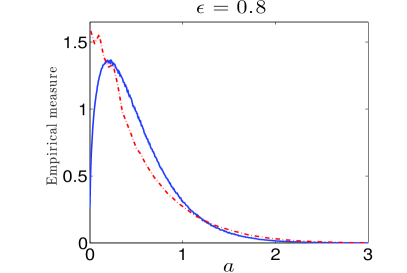
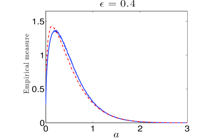
Figure 1: Probability density function (empirical measure) at $t=10$ for the fast-slow map (6.1), (6.2) with $\epsilon=0.8,0.4,0.2$ (dashed, red) and for the SDE limit (6.3) (solid, blue). We used ensembles consisting of $5,000,000$ realizations.

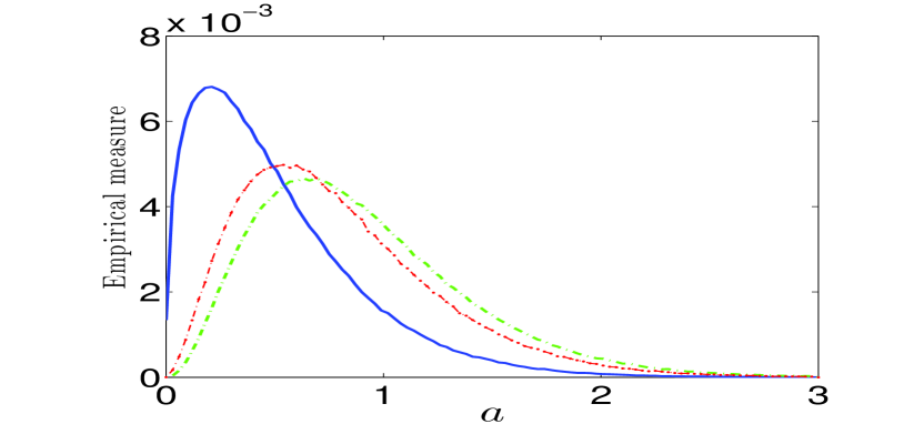
Figure 2: Probability density function (empirical measure) at $t=10$ for the limiting SDE with different drift terms corresponding to three different interpretations of the stochastic integral: the theoretically predicted drift term in (6.3) (left, blue) and those for the Itô interpretation (middle, red) and the Stratonovich interpretation (right, green). We used ensembles consisting of $5,000,000$ realizations.

We also present numerical evidence for convergence of first moments ${\mathbb{E}}(|\hat{x}^{(\epsilon)}(t)|)$. This is not a direct consequence of Theorem 1.3. However, for each $t>0$, Theorem 1.3 together with boundedness (as $\epsilon$ varies) of a higher moment implies (eg. [8, Exercise 2.5, p. 86] that ${\mathbb{E}}(|\hat{x}^{(\epsilon)}(t)|)$ converges, as $\epsilon\to 0$, to

$${\mathbb{E}}(X(t))=\xi e^{-\alpha t}+\beta(1-e^{-\alpha t}).$$ (6.5)

We verified numerically that ${\mathbb{E}}((\hat{x}^{(\epsilon)}(t))^{2})$ is convergent and hence bounded, implying convergence of ${\mathbb{E}}(|\hat{x}^{(\epsilon)}(t)|)$ as demonstrated in Figure 3.

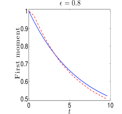
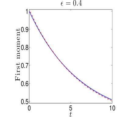
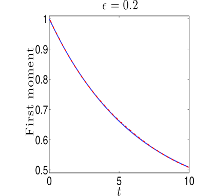
Figure 3: First moment $0\leq t\leq 15$ for the fast-slow map (6.1), (6.2) with $\epsilon=0.8,0.4,0.2$ (dashed, red) and for the SDE limit (6.5) (solid, blue). We used ensembles consisting of $100,000$ realizations for the fast-slow map.

7 Conclusions

The paper [21] set out a programme for a rigorous investigation of homogenisation for fast-slow deterministic systems under very mild assumptions on the fast dynamics. In this paper, we have extended these results in a number of ways:

• Extension from continuous time to discrete time.

• Incorporation of one-dimensional multiplicative noise.

• Inclusion of situations where the SDE is driven by a stable Lévy process.

• Relaxation of regularity assumptions, in particular the requirement in [21] that certain vector fields are uniformly Lipschitz.

Items 2–4 require interpretation of certain stochastic integrals. In the case of multiplicative noise in continuous time, the stochastic integrals are of Stratonovich type as would be expected. For discrete time, it was pointed out in [9] that the integrals are neither Itô nor Stratonovich. We recover their result in a much more general context. For multiplicative noise in the situation of item 3, where the SDE is Lévy, we obtain Marcus stochastic integrals for both discrete and continuous time.

Important directions of future research include the analysis of higher-dimensional multiplicative noise and of fully coupled systems where the fast dynamics depends on the slow variables.

Appendix A Averaging argument

Let $K_{2}^{(\epsilon)}$ be the expression appearing in the proof of Theorem 1.1 in Subsection 4.1. For completeness, we give the details of the argument that $K_{2}^{(\epsilon)}\to 0$ in probability in $D([0,T],{\mathbb{R}}^{d})$. The proof is identical to that in the continuous time context in [21]. (Note that the published version of [21] contains an error that is corrected in the updated version on arXiv. The published version of our paper replicated this error which is corrected in identical fashion below.)

Lemma A.1

$K_{2}^{(\epsilon)}\to 0$ in probability in $D([0,T],{\mathbb{R}}^{d})$.

Proof.

Define $\tilde{f}(x,y)=f(x,y,0)-F(x)$ and note that $|\tilde{f}|_{\infty}\leq 2|f|_{\infty}$ and $\operatorname{Lip}(\tilde{f})\leq 2\operatorname{Lip}(f)$. Then $K_{2}^{(\epsilon)}(t)=\epsilon^{2}\sum_{0\leq j<[t\epsilon^{-2}]}\tilde{f}(x^{(\epsilon)}(j),y(j))$. Let $N=[t/\epsilon^{3/2}]$ and write $K_{2}^{(\epsilon)}(t)=K_{2}^{(\epsilon)}(N\epsilon^{3/2})+I_{0}$ where $I_{0}=\epsilon^{2}\sum_{N\epsilon^{-1/2}\leq j<t\epsilon^{-2}}\tilde{f}(x^{(\epsilon)}(j),y(j))$. We have

$$|I_{0}|\leq(t-N\epsilon^{3/2})|\tilde{f}|_{\infty}\leq 2|f|_{\infty}\epsilon^{3/2}.$$ (A.1)

We now estimate $K_{2}^{(\epsilon)}(N\epsilon^{3/2})$ as follows:

$$K_{2}^{(\epsilon)}(N\epsilon^{3/2}) =\epsilon^{2}\sum_{n=0}^{N-1}\sum_{n\epsilon^{-1/2}\leq j<(n+1)\epsilon^{-1/2}}\tilde{f}(x^{(\epsilon)}(j),y(j))$$

$$=\epsilon^{2}\sum_{n=0}^{N-1}\sum_{n\epsilon^{-1/2}\leq j<(n+1)\epsilon^{-1/2}}\bigl{(}\tilde{f}(x^{(\epsilon)}(j),y(j))-\tilde{f}(x^{(\epsilon)}(n\epsilon^{-1/2}),y(j))\bigr{)}$$

$$\qquad\qquad+\epsilon^{2}\sum_{n=0}^{N-1}\sum_{n\epsilon^{-1/2}\leq j<(n+1)\epsilon^{-1/2}}\tilde{f}(x^{(\epsilon)}(n\epsilon^{-1/2}),y(j))$$

$$=I_{1}+I_{2}.$$

For $n\epsilon^{-1/2}\leq j<(n+1)\epsilon^{-1/2}$, we have $|x^{(\epsilon)}(j)-x^{(\epsilon)}(n\epsilon^{-1/2})|\leq(\epsilon|f_{0}|_{\infty}+\epsilon^{2}|f|_{\infty})\epsilon^{-1/2}$. Hence

$$|I_{1}| \leq N\epsilon^{3/2}\operatorname{Lip}(\tilde{f})(|f_{0}|_{\infty}+|f|_{\infty})\epsilon^{1/2}\leq 2\operatorname{Lip}(f)(|f_{0}|_{\infty}+|f|_{\infty})T\epsilon^{1/2}.$$ (A.2)

Next,

$$I_{2} =\epsilon^{2}\sum_{n=0}^{N-1}\sum_{n\epsilon^{-1/2}\leq j<(n+1)\epsilon^{-1/2}}\tilde{f}(x^{(\epsilon)}(n\epsilon^{-1/2}),y(j))=\epsilon^{3/2}\sum_{n=0}^{N-1}J_{n},$$

where

$$J_{n} =\epsilon^{1/2}\sum_{n\epsilon^{-1/2}\leq j<(n+1)\epsilon^{-1/2}}\tilde{f}(x^{(\epsilon)}(n\epsilon^{-1/2}),y(j)).$$

Hence

$$|I_{2}|\leq\epsilon^{3/2}\sum_{n=0}^{[T\epsilon^{-3/2}]-1}|J_{n}|.$$ (A.3)

For $u\in{\mathbb{R}}^{d}$ fixed, we define

$$\tilde{J}_{n}(u)=\epsilon^{1/2}\sum_{n\epsilon^{-1/2}\leq j<(n+1)\epsilon^{-1/2}}\tilde{f}(u,y(j))=\epsilon^{1/2}\sum_{n\epsilon^{-1/2}\leq j<(n+1)\epsilon^{-1/2}}A_{u}\circ g^{j}$$

where $A_{u}(y)=\tilde{f}(u,y)$. Note that $\tilde{J}_{n}(u)=\tilde{J}_{0}(u)\circ g^{[n\epsilon^{-1/2}]}$, and so ${\mathbb{E}}|\tilde{J}_{n}(u)|={\mathbb{E}}|\tilde{J}_{0}(u)|$. By the ergodic theorem, ${\mathbb{E}}|\tilde{J}_{0}(u)|\to 0$ as $\epsilon\to 0$ for each $u$.

Let $Q>0$ and write $I_{2}=M_{Q,1}+M_{Q,2}$ where

$$M_{Q,1}=I_{2}1_{B_{\epsilon}(Q)},\quad M_{Q,2}=I_{2}1_{B_{\epsilon}(Q)^{c}},\quad B_{\epsilon}(Q)=\bigl{\{}\max_{[0,T]}|x^{(\epsilon)}|\leq Q\bigr{\}}.$$

For any $a>0$, there exists a finite subset $S\subset{\mathbb{R}}^{d}$ such that $\operatorname{dist}(x,S)\leq a/(2\operatorname{Lip}(f))$ for any $x$ with $|x|\leq Q$. Then for all $n\geq 0$, $\epsilon>0$,

$$1_{B_{\epsilon}(Q)}|J_{n}|\leq\sum_{u\in S}|\tilde{J}_{n}(u)|+a.$$

Hence by (A.3),

$${\mathbb{E}}\max_{[0,T]}|M_{Q,1}| \leq\epsilon^{3/2}\sum_{n=0}^{[T\epsilon^{-3/2}]-1}\sum_{u\in S}{\mathbb{E}}|\tilde{J}_{n}(u)|+Ta$$

$$=\epsilon^{3/2}\sum_{n=0}^{[T\epsilon^{-3/2}]-1}\sum_{u\in S}{\mathbb{E}}|\tilde{J}_{0}(u)|+Ta$$

$$\leq T\sum_{u\in S}{\mathbb{E}}|\tilde{J}_{0}(u)|+Ta.$$

Since $a>0$ is arbitrary, we obtain for each fixed $Q$ that $\max_{[0,T]}|M_{Q,1}|\to 0$ in $L^{1}$, and hence in probability, as $\epsilon\to 0$.

Next, since $x^{(\epsilon)}-W^{(\epsilon)}$ is bounded on $[0,T]$, for $Q$ sufficiently large

$$\mu\bigl{\{}\max_{[0,T]}|M_{Q,2}|>0\bigr{\}}\leq\mu\bigl{\{}\max_{[0,T]}|x^{(\epsilon)}|\geq Q\bigr{\}}\leq\mu\bigl{\{}\max_{[0,T]}|W^{(\epsilon)}|\geq Q/2\bigr{\}}.$$

Fix $c>0$. Increasing $Q$ if necessary, we can arrange that $\mu\{\max_{[0,T]}|\sqrt{\Sigma}W|\geq Q/2\}<c/4$. By the continuous mapping theorem, $\max_{[0,T]}|W^{(\epsilon)}|\to_{d}\max_{[0,T]}|\sqrt{\Sigma}W|$. Hence there exists $\epsilon_{0}>0$ such that $\mu\{\max_{[0,T]}|W^{(\epsilon)}|\geq Q/2\}<c/2$ for all $\epsilon\in(0,\epsilon_{0})$. For such $\epsilon$,

$$\mu\bigl{\{}\max_{[0,T]}|M_{Q,2}|>0\bigr{\}}<c/2.$$

Shrinking $\epsilon_{0}$ if necessary, we also have that $\mu\{\max_{[0,T]}|M_{Q,1}|>c/2\}<c/2$. Hence $\mu\{\max_{[0,T]}|I_{2}|>c\}<c$, and so $\max_{[0,T]}|I_{2}|\to 0$ in probability. Combining this with estimates (A.1) and (A.2), we obtain that $\max_{[0,T]}|K_{2}^{(\epsilon)}|\to 0$ in probability as required. ∎

Acknowledgements

The research of GAG was supported in part by ARC grant FT 0992214. The research of IM was supported in part by EPSRC Grant EP/F031807/1 held at the University of Surrey. IM is grateful to the hospitality at the University of Sydney where this research commenced in 2011. We are grateful to Ben Goldys, David Kelly and especially Andrew Stuart for helpful discussions, and also to the referees for several helpful comments and suggestions.

References

• [1] D. Applebaum. Lévy processes and stochastic calculus, second ed. Cambridge Studies in Advanced Mathematics 116, Cambridge University Press, Cambridge, 2009.
• [2] C. Beck. Brownian motion from deterministic dynamics. Phys. A 169 (1990) 324–336.
• [3] P. Billingsley. Convergence of probability measures, second ed., Wiley Series in Probability and Statistics: Probability and Statistics, John Wiley & Sons Inc., New York, Wiley-Interscience Publication, 1999.
• [4] R. Bowen. Equilibrium States and the Ergodic Theory of Anosov Diffeomorphisms. Lecture Notes in Math. 470, Springer, Berlin, 1975.
• [5] R. Bowen and D. Ruelle. The ergodic theory of Axiom A flows. Invent. Math. 29 (1975) 181–202.
• [6] J. C. Cox, J. E. Ingersoll and S. Ross. An inter temporal general equilibrium model of asset prices. Econometrica 53 (1985) 363–384.
• [7] J. C. Cox, J. E. Ingersoll and S. Ross. A theory of the term structure of interest rates. Econometrica 53 (1985) 385–407.
• [8] R. Durrett. Probability: theory and examples, third ed., Duxbury Press, Belmont, CA, 1996.
• [9] D. Givon and R. Kupferman. White noise limits for discrete dynamical systems driven by fast deterministic dynamics. Phys. A 335 (2004) 385–412.
• [10] S. Gouëzel. Central limit theorem and stable laws for intermittent maps. Probab. Theory Relat. Fields 128 (2004) 82–122.
• [11] W. Just, H. Kantz, C. Rödenbeck and M. Helm. Stochastic modelling: replacing fast degrees of freedom by noise. J. Phys. A 34 (2001) 3199–3213.
• [12] R. Kupferman, G. A. Pavliotis and A. M. Stuart. Itô versus Stratonovich white-noise limits for systems with inertia and colored multiplicative noise. Phys. Rev. E (3) 70 (2004) 036120, 9.
• [13] T. G. Kurtz, E. Pardoux and P. Protter. Stratonovich stochastic differential equations driven by general semimartingales. Ann. Inst. H. Poincaré Probab. Statist. 31 (1995) 351–377.
• [14] C. Liverani, B. Saussol and S. Vaienti. A probabilistic approach to intermittency. Ergodic Theory Dynam. Systems 19 (1999) 671–685.
• [15] S. I. Marcus. Modeling and approximation of stochastic differential equations driven by semimartingales. Stochastics 4 (1980/81) 223–245.
• [16] A. J. Majda and I. Timofeyev. Remarkable statistical behavior for truncated Burgers-Hopf dynamics. Proc. Natl. Acad. Sci. USA 97 (2000) 12413–12417.
• [17] A. M. Majda, I. Timofeyev, and E. Vanden-Eijnden. Stochastic models for selected slow variables in large deterministic systems. Nonlinearity 19 (2006) 769–794.
• [18] R. S. Mackay. Langevin equation for slow degrees of freedom of Hamiltonian systems. In: Nonlinear Dynamics and Chaos: Advances and Perspectives (Understanding Complex Systems). pp. 89–102, Berlin, Springer, 2010.
• [19] I. Melbourne and M. Nicol. Almost sure invariance principle for nonuniformly hyperbolic systems. Commun. Math. Phys. 260 (2005) 131–146.
• [20] I. Melbourne and M. Nicol. A vector-valued almost sure invariance principle for hyperbolic dynamical systems. Ann. Probability 37 (2009) 478–505.
• [21] I. Melbourne and A. Stuart. A note on diffusion limits of chaotic skew product flows. Nonlinearity (2011) 1361–1367. Updated version at arXiv:1101.3087.
• [22] I. Melbourne and A. Török. Convergence of moments for Axiom A and nonuniformly hyperbolic flows. Ergodic Theory Dynam. Systems 32 (2012) 1091–1100.
• [23] I. Melbourne and R. Zweimüller. Weak convergence to stable Lévy processes for nonuniformly hyperbolic dynamical systems. Preprint, 2013.
• [24] G. A. Pavliotis and A. M. Stuart. Analysis of white noise limits for stochastic systems with two fast relaxation times. Multiscale Model. Simul. 4 (2005) 1–35.
• [25] G. A. Pavliotis and A. M. Stuart. Multiscale methods: Homogenization and Averaging. Texts in Applied Mathematics 53, Springer, New York, 2008.
• [26] Y. Pomeau and P. Manneville. Intermittent transition to turbulence in dissipative dynamical systems. Comm. Math. Phys. 74 (1980) 189–197.
• [27] D. Ruelle. Thermodynamic Formalism. Encyclopedia of Math. and its Applications 5, Addison Wesley, Massachusetts, 1978.
• [28] G. Samorodnitsky and M. S. Taqqu. Stable non-Gaussian random processes. Stochastic Modeling, Chapman & Hall, New York, 1994.
• [29] Y. G. Sinaĭ. Gibbs measures in ergodic theory. Russ. Math. Surv. 27 (1972) 21–70.
• [30] H. J. Sussmann. On the gap between deterministic and stochastic ordinary differential equations. Ann. Probability 6 (1978) 19–41.
• [31] E. Wong and M. Zakai. On the convergence of ordinary integrals to stochastic integrals. Ann. Math. Statist. 36 (1965) 1560–1564.
• [32] L.-S. Young. Statistical properties of dynamical systems with some hyperbolicity. Ann. of Math. 147 (1998) 585–650.
• [33] L.-S. Young. Recurrence times and rates of mixing. Israel J. Math. 110 (1999) 153–188.