Intermittency in spherical Couette dynamos

Abstract

We investigate dynamo action in three-dimensional numerical simulations of turbulent spherical Couette flows. Close to the onset of dynamo action, the magnetic field exhibits an intermittent behavior, characterized by a series of short bursts of the magnetic energy separated by low-energy phases. We show that this behavior corresponds to the so-called on-off intermittency. This behavior is here reported for dynamo action with realistic boundary conditions. We investigate the role of magnetic boundary conditions in this phenomenon.

I Introduction

First suggested by Joseph Larmor in 1919, dynamo action, i.e. the self-amplification of a magnetic field by the flow of an electrically conducting fluid, is considered to be the main mechanism for the generation of magnetic fields in the universe for a variety of systems, including planets, stars, and galaxies Dormy, E. and Soward, A. M. (2007). Dynamo action is an instability by which a conducting fluid transfers part of its kinetic energy to magnetic energy.

In experiments, it is rather difficult to achieve a regime of self-excited dynamo action. The low value of the magnetic Prandtl number of liquid metals requires the injection of a sufficiently high mechanical power, and thus generates turbulent flows, before reaching the dynamo threshold. Dynamo action was first observed experimentally only in 2001, in Karlsruhe Stieglitz and Müller (2001) and Riga Gailitis et al. (2001), and then in 2007 with a von Kármán swirling flow of liquid sodium Monchaux et al. (2007).

In parallel with these approaches, numerical simulations have been carried out to model either laboratory experiments or astrophysical systems, for which the spherical geometry is relevant. We investigate spherical Couette flow and focus on the characteristics of the magnetic field close to the dynamo onset. We observe a series of short bursts of the magnetic energy separated by low-energy phases. This intermittent behavior, also known as on-off intermittency or blowout bifurcation, is usually interpreted as the effect of a multiplicative noise acting on a bifurcating system Fujisaka and Yamada (1986); Platt et al. (1993).

On-off intermittency has so far never been observed in dynamo experiments, except in the case of an externally amplified magnetic field Verhille et al. (2010). In contrast, it has been reported in a small number of numerical simulations Sweet et al. (2001); Leprovost et al. (2006); Alexakis and Ponty (2008), all relying on a flow in a periodic geometry produced by a periodic analytic forcing. Here we investigate the influence of a realistic choice of boundary conditions on this phenomenon.

II Governing equations

The spherical Couette flow geometry consists of two concentric spheres in differential rotation: the outer sphere, of radius $r_{\text{o}}$, is rotating around the vertical axis $\mathbf{e}_{\text{z}}$ with an angular velocity $\Omega$, and the solid inner sphere, of radius $r_{\text{i}}$, is rotating at velocity $\Omega+\Delta\Omega$ around an axis that can make an angle $\theta$ with $\mathbf{e}_{\text{z}}$. The aspect ratio $\chi=r_{\text{i}}/r_{\text{o}}$ is set to 0.35 to mimic that of Earth’s liquid core. The spherical shell in between the two spheres is filled with an incompressible conducting fluid of kinematic viscosity $\nu$, electrical conductivity $\sigma$, and density $\rho$. Its magnetic permeability $\mathrm{\mu}_{0}$ is that of vacuum. The magnetic diffusivity $\eta$ is defined as $\eta=1/(\mathrm{\mu}_{0}\sigma)$.

We describe the problem in the reference frame rotating with the outer sphere. This introduces two extra terms in the governing equations: the Coriolis force and the centrifugal acceleration. The latter can be rewritten in the form $\tfrac{1}{2}\nabla\left(\Omega^{2}s^{2}\right)$, where $s$ denotes the distance to the axis of rotation. This term is a gradient and can be added to the pressure term which acts as a Lagrange multiplier to enforce the solenoidal condition on the velocity field. To establish the set of equations for this system, we rely on the same non-dimensional form as in Guervilly and Cardin (2010): the velocity $\mathbf{u}$ is scaled by $r_{\text{i}}\Delta\Omega$, the magnetic field $\mathbf{B}$ by $\sqrt{\rho\mathrm{\mu}_{0}r_{\text{i}}r_{\text{o}}\left(\Omega+\Delta\Omega\right)\Delta\Omega}$, and the length scale by $r_{\text{o}}$. The Navier-Stokes equation governing the fluid velocity $\mathbf{u}$ then takes the form

$$\frac{\partial\,\mathbf{u}}{\partial t}+\left(\mathbf{u}\cdot\nabla\right)\mathbf{u}+\frac{2}{\mathrm{E}\mathrm{Re}}\left(\mathbf{e}_{\text{z}}\times\mathbf{u}\right)=-\frac{1}{\mathrm{Re}}\nabla\Pi+\\ \frac{1}{\mathrm{Re}}\mathbf{\nabla^{2}}\mathbf{u}+\frac{1}{\mathrm{Re}}\left(\frac{1}{\mathrm{E}}+\frac{\mathrm{Re}}{\chi}\right)\left(\nabla\times\mathbf{B}\right)\times\mathbf{B}\,,$$ (1)

and the induction equation for the magnetic field $\mathbf{B}$,

$$\frac{\partial\,\mathbf{B}}{\partial t}=\nabla\times\left(\mathbf{u}\times\mathbf{B}\right)+\frac{1}{\mathrm{Rm}}\mathbf{\nabla^{2}}\mathbf{B}\,.$$ (2)

Both fields are solenoidal

$$\nabla\cdot\mathbf{u}=0\,,\qquad\nabla\cdot\mathbf{B}=0\,.$$ (3)

The dimensionless parameters are the Ekman number $\mathrm{E}=\nu/\left(\Omega r_{\text{o}}^{2}\right)$, the Reynolds number $\mathrm{Re}=\left(r_{\text{o}}r_{\text{i}}\Delta\Omega\right)/\nu$, the magnetic Prandtl number $\mathrm{P_{m}}=\nu/\eta$, and the magnetic Reynolds number $\mathrm{Rm}=\mathrm{Re}\mathrm{P_{m}}$. The potential $\Pi$ includes all gradient terms (the pressure term as well as the centrifugal effect introduced above). The Reynolds number varies with the rotation rate of the inner sphere, while the Ekman number is inversely proportional to the rotation rate of the outer sphere. When the latter is at rest, the Ekman number tends toward infinity and the Coriolis term in the Navier-Stokes equation vanishes. In our simulations, the Ekman number is set to $10^{-3}$. This moderate value yields a moderate computing time.

We impose no slip boundary conditions for the velocity field on both spheres. Magnetic boundary conditions are of three types. The first one can only be applied to the inner sphere, as it implies a meshing of the bounding solid domain. The inner sphere can be a conductor with the same electric and magnetic properties as the fluid. In that case the magnetic diffusion equation is discretized and solved in the solid conductor (we refer to this set of boundary conditions as “conducting”). The outer sphere as well as the inner sphere can be electrical insulators. In that case the magnetic field is continuous across the boundary and matches a potential field, decaying away from the boundary. The spherical harmonic expansion allows an explicit and local expression for these boundary conditions (we refer to these boundary conditions as “insulating”). In addition, the use of high-magnetic-permeability boundary conditions may enhance dynamo action Gissinger et al. (2008). Therefore, we also used boundary conditions which enforce the magnetic field to be normal to the boundary. This is equivalent to assuming that the medium on the other side of the boundary has an infinitely larger permeability (we refer to these boundary conditions as “ferromagnetic”). The different configurations investigated in this study are summarized in Table 1.

	Inner Sphere	Outer Sphere
B.C.1	Conducting	Insulating
B.C.2	Insulating	Insulating
B.C.3	Ferromagnetic	Ferromagnetic

TABLE. 1: The three different configurations of magnetic boundary conditions used in this study.

We integrated our system with parody Dormy et al. (1998), a parallel code which has been benchmarked against other international codes. The vector fields are transformed into scalars using the poloidal-toroidal decomposition. This expansion on a solenoidal basis enforces the constraints (3). The equations are then discretized in the radial direction with a finite-difference scheme on a stretched grid. On each concentric sphere, variables are expanded using a spherical harmonic basis (i.e., generalized Legendre polynomials in latitude and a Fourier basis in longitude). The coefficients of the expansion are identified with their degree $l$ and order $m$. The simulations were performed using from 150 to 216 points in the radial direction, and the spherical harmonic decomposition is truncated at $(l_{\text{max}},m_{\text{max}})=(70,20)$. We observe for both spectra a decrease of more than two orders of magnitude over the range of $l$ and $m$. This provides an empirical validation of convergence. We checked on a few critical cases that the results are not affected when the resolution is increased to $l_{\text{max}}=100\,$.

Let us define the non-dimensional kinetic and magnetic energy densities as

$$E_{k}=\frac{1}{V_{s}}\int_{V_{s}}\mathbf{u}^{2}{\rm d}\mathbf{x}\,,$$ (4)

$$E_{b}=\frac{1}{V_{s}}\,\frac{1}{\mathrm{Re}}\left(\frac{1}{\mathrm{E}}+\frac{\mathrm{Re}}{\chi}\right)\,\int_{V_{s}}\mathbf{B}^{2}{\rm d}\mathbf{x}\,,$$ (5)

in which the unit of energy density is $\rho\left(r_{i}\,\Delta\Omega\right)^{2}$. In the above expressions, $V_{s}$ refers to the volume of the spherical shell. In addition, we also investigate the symmetry of the flow and the symmetry of the magnetic field with respect to the equatorial plane. To that end, we define the contributions to the energy densities corresponding to the symmetric and antisymmetric components of the velocity (respectively $E_{kS}$ and $E_{kA}$) and magnetic field (respectively $E_{bS}$ and $E_{bA}$). The symmetric and antisymmetric contributions to the kinetic energy density respectively correspond to the flows

$$\mathbf{u}_{S}(x,y,z)=\tfrac{1}{2}\left[\mathbf{u}(x,y,z)+\mathbf{u}(x,y,-z)\right],$$ (6)

$$\mathbf{u}_{A}(x,y,z)=\tfrac{1}{2}\left[\mathbf{u}(x,y,z)-\mathbf{u}(x,y,-z)\right].$$ (7)

In contrast, the symmetries are reversed for the magnetic field. This comes from the fact that the magnetic field is a pseudovector (i.e, the curl of a vector). Then,

$$\mathbf{B}_{S}(x,y,z)=\tfrac{1}{2}\left[\mathbf{B}(x,y,z)-\mathbf{B}(x,y,-z)\right],$$ (8)

$$\mathbf{B}_{A}(x,y,z)=\tfrac{1}{2}\left[\mathbf{B}(x,y,z)+\mathbf{B}(x,y,-z)\right].$$ (9)

According to our definition, the dipolar component is symmetric.

III Direct numerical simulations

As shown by Guervilly and Cardin (2010), contra-rotation is more efficient than co-rotation for dynamo action. In order to introduce more control over the system, we let the angle $\theta$ between the axes of rotation of both spheres take any value in $\left[0,\pi\right]$. Contrary to our expectations, we do not significantly lower the dynamo threshold with the inclination of the rotation axis of the inner sphere. In fact, for $\theta=\pi/2$, the fluid is mainly in co-rotation with the outer sphere, and dragged only by a thin layer on the inner sphere, which is not sufficient to trigger dynamo action. In our parameter regime, the best configuration seems to remain $\theta=\pi$, when the two spheres are in contra-rotation. We therefore keep this parameter fixed in the rest of the study.

III.1 Role of boundary conditions

Let us first investigate the dynamo transition in this setup at fixed magnetic Prandtl number $\mathrm{P_{m}}=0.2$, using the Reynolds number as the controlling parameter. With a conducting inner sphere and an insulating outer sphere, we find a critical magnetic Reynolds number $\mathrm{Rm}_{\text{c}}\in[291.0;292.0]$, which is in good agreement with Guervilly and Cardin (2010). Above the dynamo onset, the magnetic field displays an intermittent behavior characterized by series of short bursts of the magnetic energy separated by low energy phases (see Fig. 1). When the distance to the threshold increases, bursts become more and more frequent and eventually intermittency disappears.

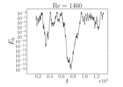
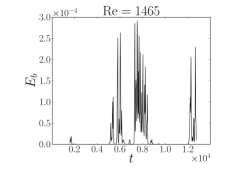
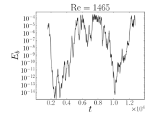
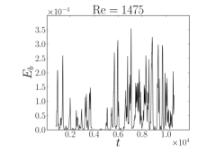
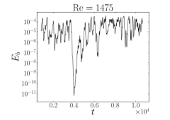
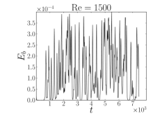
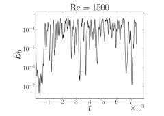
FIG. 1: Time evolution of the magnetic energy in linear (left) and log scale (right) for increasing Reynolds numbers at $\mathrm{P_{m}}=0.2$, using a conducting inner sphere (B.C.1 in Table 1). At lower Reynolds numbers (top), we see in linear scale the characteristic intermittent bursting. Intermittency gradually disappears at higher Reynolds numbers and the field reaches saturation.

Changing the boundary conditions generally leads to different thresholds for dynamo action. Using ferromagnetic boundary conditions, we find a critical magnetic Reynolds number $\mathrm{Rm}_{\text{c}}\in[298.6;300.0]$. With insulating boundary conditions, the threshold becomes large and involves larger numerical resolutions. In order to maintain the hydrodynamic Reynolds number at values which involve a moderate resolution, we therefore had to increase the magnetic Prandtl number from 0.2 to $0.4\,$. We then obtain the dynamo onset for $\mathrm{Rm}_{\text{c}}\in[530.0;534.8]\,$. We emphasize that we observe the same intermittent regime with all the above choices of boundary conditions as long as the magnetic Reynolds number is close enough to the onset of the instability.

For all boundary conditions, we observe that the dominant mode is predominantly of quadrupolar symmetry [the larger poloidal and toroidal modes are the $(l=2,m=0)$ and $(l=1,m=0)$ modes, respectively]. For these Reynolds numbers, the flow is predominantly equatorially symmetric ($E_{kA}\ll E_{kS}$).

III.2 Increasing the magnetic Prandtl number

Having assessed that the intermittent behavior of the magnetic field near onset could be observed with three different sets of boundary conditions, we restrict here our attention to simulations with ferromagnetic boundary conditions.

Figure 2 presents the results we obtain at $\mathrm{P_{m}}=2\,$. Close to the threshold, the magnetic field still exhibits intermittency, but the nature of the process has significantly changed. There is now a clear distinction between two different regimes: phases of dynamo activity separated by phases of pure exponential decay. Both seem to alternate randomly. When the dynamo is active, the magnetic field still displays a quadrupolar symmetry. In contrast, we observe the emergence of an axial dipole during decaying phases. The change of the global symmetry of the field coincides with the change of slope in the decaying phases [see Fig. 2 (bottom) and Fig. 3]. This change of slope is associated with a slower decay of the dipolar component over the quadrupolar mode.

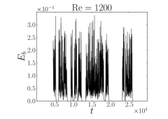
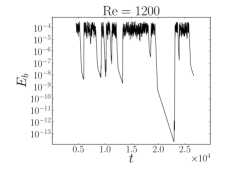
FIG. 2: Time evolution of the magnetic energy in linear and log scales for $\mathrm{P_{m}}=2$ and $\mathrm{Re}=1200$, using ferromagnetic boundary conditions. Instead of bursts, we now observe phases of dynamo activity which seem to randomly alternate with phases of exponential decay. The latter are no longer chaotic and are instead characterized by two different decay rates.

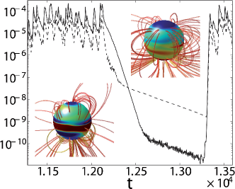
FIG. 3: (Color online) Time evolution of the symmetric (dashed line) and antisymmetric (solid line) part of the magnetic energy. We focus on one of the decaying phases presented in Fig. 2. The decaying phase is characterized by a change of the dominant symmetry, as we can see on the visualizations of the magnetic field lines. The color insets respectively correspond to snapshots in the quadrupolar phase (left) and dipolar phase (right).

IV Discussion

IV.1 Canonical model for on-off intermittency

The simplest model that exhibits on-off intermittency is Aumaître et al. (2005)

$$\dot{X}=\left[a+\zeta(t)\right]X-X^{3}\,,$$ (10)

where $a$ is the distance to the threshold, and $\zeta$ a Gaussian white noise of zero mean value and amplitude $D$, defined as $\langle\zeta(t)\zeta(t^{\prime})\rangle=D\delta(t-t\textquoteright)$ where $\langle\rangle$ indicates the average over realizations (ensemble average). In the absence of noise, the system undergoes a supercritical pitchfork bifurcation at $a=0\,$. If $a$ is sufficiently small, the fluctuations lead to on-off intermittency, with bursts ($a+\zeta>0$) followed by decays ($a+\zeta<0$). During the off phases, one can neglect nonlinearities and write $\dot{Y}=a+\zeta(t)$, with $Y=\ln(X)$. Thus, $\ln(X)$ should follow a random walk, with a small positive bias. Since solutions of Eq. (10) mimic solutions of the magnetohydrodynamics equations we observe in Fig. 1, we further investigate some properties of the model. (i) Equation (10) leads to a stationary probability density function (PDF) of the form Stratonovitch (1963)

$$P(X)\propto X^{(2a/D)-1}e^{-X^{2}/D}\,,$$ (11)

which diverges at the origin for $0\leqslant s=(2a/D)-1<1\,$. (ii) In addition, all the moments of $X$ must follow a linear scaling with $a$. (iii) Finally, another characteristic of this model is that the distribution of the duration of the off phases $T_{\text{off}}$ follows a power law behavior, $P(T_{\text{off}})\sim T_{\text{off}}^{-\alpha}$, with $\alpha=-3/2$. To compare these predictions to our results, we rely as in Alexakis and Ponty (2008) on the magnetic energy density as a global measure of the magnetic field strength.

IV.2 Predictions and results

Figure 4 shows the PDFs of the magnetic energy for a set of simulations at different Reynolds numbers.

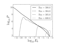
FIG. 4: Estimates of the probability density functions. Statistics are done from time series of the magnetic energy obtained with ferromagnetic boundary conditions, for $\mathrm{P_{m}}=0.2$.

At low $\mathrm{Rm}$, the PDF is characterized by a linear scaling on a log-log plot. The cutoff at low energies is not predicted by the theory, which considers the limit $E_{\text{b}}\to 0\,$. For $\mathrm{Rm}>310\,$, the magnetic energy fluctuates around a mean value and the PDF no longer scales as a power law. We see in Fig. 5 that the coefficient $s$ is proportional to the distance to the threshold.

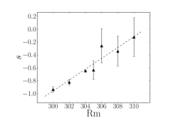
FIG. 5: Fit of the coefficient $s=(2a/D)-1$, taking into account the linear domain of the PDFs in the intermittent regime only. Statistics are done from time series of the magnetic energy obtained with ferromagnetic boundary conditions, for $\mathrm{P_{m}}=0.2$.

Examples of the fit of the exponent $s$ are presented in Fig. 6.

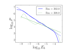
FIG. 6: (Color online) Examples of the fit (dashed lines) of the probability density functions (solid and dotted lines). Statistics are done from time series of the magnetic energy obtained with ferromagnetic boundary conditions, for $\mathrm{P_{m}}=0.2$.

The values of the coefficient are mainly affected by the range over which the data are fitted. Thus we select a range as large as possible. We then randomly sample this range with half-size sub-intervals. We then compute the mean slope and its standard deviation (represented in Fig. 5 with error bars).

We then investigate the linearity of the moments. Figure 7 shows our results for the first and second moments of the magnetic energy. We see that the mean magnetic energy grows linearly as a function of the magnetic Reynolds number. The second moments seem to follow the same linear trend, but only at the lower values of the magnetic Reynolds number. Deviations at larger values of $\mathrm{Rm}$ are expected, as this description is only valid in the limit $\mathrm{Rm}\to\mathrm{Rm}_{\text{c}}\,$. The duration $t_{I}$ of the time series used to compute these values ranges from $3.2\,10^{3}$ to $1.4\,10^{4}$ U.T. (values are presented in Table 2). These integration times are quite significant for a fully three dimensional set of partial differential equations but are necessarily short compared to the ones usually used with simplified models such as Eq. (10). To quantify the uncertainty associated with the moment values, we sampled the integration time with sub-intervals randomly chosen. We then computed the moments on the full interval (symbols in Fig. 7) and the standard deviation on the sub-intervals (reported as error bars). The sub-intervals can be set from $t_{I}/4$ to $t_{I}/10$ without affecting these estimates.

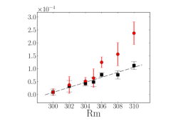
FIG. 7: (Color online) Moments of the magnetic energy as function of the magnetic Reynolds number. Black squares represent the mean. The dashed line fits these data points with an error about 10% on the slope coefficient. The second moments (red circles) have been rescaled to match with the mean at $\mathrm{Rm}=300\,$.

$\mathrm{Rm}$	$t_{I}$	$t_{I}/\mathrm{Rm}$
300	$1.40\,10^{4}$	46.7
302	$9.06\,10^{3}$	30.0
304	$9.05\,10^{3}$	29.8
305	$3.33\,10^{3}$	10.9
306	$7.58\,10^{3}$	24.8
308	$3.20\,10^{3}$	10.4
310	$5.46\,10^{3}$	17.6

TABLE. 2: Duration of the time series used to compute the moments of the magnetic energy. The integration time $t_{I}$ is presented in units of $\left(\chi\Delta\Omega\right)^{-1}$ ($t_{I}$) and in units of the magnetic diffusion time $r_{\text{o}}^{2}/\eta$ ($t_{I}/\mathrm{Rm}$).

Finally, we also tested the distribution of the duration time of the off phases. A definitive validation would require longer simulations, in order to have a significant number of off phases. For this reason, we can not rely on the simulations immediately above the threshold. Despite these short-comings, an illustrative case is presented in Fig. 8. Numerical values are given in Table 3.

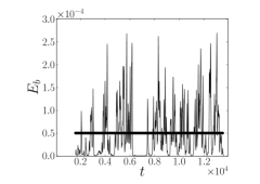
(a) (b)

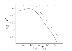
FIG. 8: Distribution of the duration of the off phases for a simulation performed at $\mathrm{P_{m}}=0.2$ and $\mathrm{Re}=1470$, with conducting boundary conditions. We define an off phase by a magnetic energy below a threshold value (indicated here by the horizontal black line). The PDF (b) decay is close to a power law with the expected $-3/2$ value for the exponent (dashed line).

	[1.7 ; 3]	[2.0 ; 3]	[2.1 ; 3]
$1.1\,10^{-4}$	-1.30	-1.48	-1.51
$1.0\,10^{-4}$	-1.35	-1.48	-1.50
$7.5\,10^{-5}$	-1.40	-1.41	-1.40
$5.0\,10^{-5}$	-1.48	-1.52	-1.51
$3.5\,10^{-5}$	-1.51	-1.60	-1.65

TABLE. 3: Estimate of the exponent $\alpha$ of the PDF of the duration of the off phases for different threshold values and different ranges over which the fit is done. The standard error on the estimate of $\alpha$ is about $1\%$. Range values correspond to $\log_{10}T_{\text{off}}$ [x axis in Fig. 8(b)].

To conclude, we emphasize that the predictions of the model are consistent with the three-dimensional simulations, and thus confirm the on-off hypothesis for the observed intermittency at low magnetic Prandtl number.

IV.3 Simulations at higher magnetic Prandtl number

The simulations we performed at $\mathrm{P_{m}}=2$ exhibit a peculiar behavior of the magnetic field. This can be better understood by examining the dynamics of the flow. Indeed, we also carried out purely hydrodynamic simulations at $\mathrm{Re}=1200$ and observed intermittent transitions between two states. This kind of intermittent behavior of the flow was not reported in Guervilly and Cardin (2010), but has been observed experimentally Zimmerman et al. (2011). One state is characterized by larger fluctuations of the energy as we can see in Fig. 9.

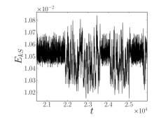
FIG. 9: Time evolution of the symmetric part of the kinetic energy $E_{kS}$ at $\mathrm{Re}=1200$ in a purely hydrodynamic simulation. Intermittent transitions between “laminar” and more turbulent phases are clearly visible.

In addition, the analysis of the energy spectra reveals that the $m=3$ modes dominate over the $m=2$ modes during the “laminar” phases, whereas both are of the same order during the “turbulent” phases. Duration of the “turbulent” phases tends to increase gradually with the increase of the Reynolds number, so that the intermittent behavior of the flow eventually disappears and is thus no longer present in the simulations at higher Reynolds number in which we have identified on-off intermittency.

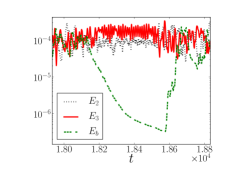
FIG. 10: (Color online) Time evolution at $\mathrm{Re}=1200$ and $\mathrm{P_{m}}=2$ of the total magnetic energy $E_{b}$ (dashed green line) and the kinetic energies $E_{2}$ (dotted black line) and $E_{3}$ (solid red line) for the $m=2$ and $m=3$ modes, respectively. When the latter becomes larger than the former, the dynamo is no longer sustained and the magnetic energy exponentially decays.

Dynamo action is inhibited during the “laminar” phases (when the $m=3$ modes dominate), which highlights the mechanism which leads to the peculiar behavior of the magnetic field, as we can see in Fig. 10. In contrast, “turbulent” phases favor dynamo action, and one must wait a change in the flow to see the restart of dynamo action after a phase of decay. Moreover, in a full magnetohydrodynamics simulation, we can artificially suppress the $m=3$ modes of the velocity field by setting them equal to zero at each time step. We check that it is sufficient to suppress intermittency of the flow. Then, we observe that the phases of exponential decay are also suppressed and the dynamo is no longer intermittent.

V Conclusion

Despite the fact that on-off intermittency has so far never been observed in dynamo experiments, we showed that the phenomenon can appear in numerical simulations of dynamo action using realistic boundary conditions. We identified in several cases the predicted behavior of the PDF of the magnetic energy, linear scaling of the moments, and distribution of the duration of the off phases. In addition, we tested these properties for three different boundary conditions (conducting inner core with insulating outer sphere, insulating or ferromagnetic spheres). Finally, we pointed out a different kind of intermittency due to hydrodynamic transitions that appears at lower Reynolds numbers.

To explain the absence of on-off intermittency in the experiments, several reasons have already been invoked Pétrélis et al. (2007). One explanation could be the imperfectness of the bifurcation (due for instance to Earth’s ambient magnetic field). Since it has been shown that low-frequency noise controls on-off intermittency Aumaître et al. (2005), another possible explanation could be that the low-frequency fluctuations are too small. However, the lack of experimental observations of on-off intermittency remains an open question and needs further investigations.