The local-global conjecture for scheduling with non-linear cost

Abstract

We consider the classical scheduling problem on a single machine, on which we need to schedule sequentially $n$ given jobs. Every job $j$ has a processing time $p_{j}$ and a priority weight $w_{j}$, and for a given schedule a completion time $C_{j}$. In this paper we consider the problem of minimizing the objective value $\sum_{j}w_{j}C_{j}^{\beta}$ for some fixed constant $\beta>0$. This non-linearity is motivated for example by the learning effect of a machine improving its efficiency over time, or by the speed scaling model. For $\beta=1$, the well-known Smith’s rule that orders job in the non-increasing order of $w_{j}/p_{j}$ give the optimum schedule. However, for $\beta\neq 1$, the complexity status of this problem is open. Among other things, a key issue here is that the ordering between a pair of jobs is not well-defined, and might depend on where the jobs lie in the schedule and also on the jobs between them. We investigate this question systematically and substantially generalize the previously known results in this direction. These results lead to interesting new dominance properties among schedules which lead to huge speed up in exact algorithms for the problem. An experimental study evaluates the impact of these properties on the exact algorithm A*.

1 Introduction

In a typical scheduling problem we have to order $n$ given jobs, each with a different processing time, so to minimize some problem specific cost function. Every job $j$ has a positive processing time $p_{j}$ and a priority weight $w_{j}$. A schedule is defined by a ranking $\sigma$, and the completion time of job $j$ is defined as $C_{j}:=\sum_{i}p_{i}$, where the sum ranges over all jobs $i$ such that $\sigma_{i}\leq\sigma_{j}$. The goal is to produce a schedule that minimizes some cost function involving the jobs’ weights and the completion times.

A popular objective function is the weighted average completion time $\sum w_{j}C_{j}$ (omitting the normalization factor $1/n$). It has been known since the 1950’s that optimal schedules are precisely the orders following an decreasing Smith-ratio $w_{j}/p_{j}$, as has been shown by a simple exchange argument (Smith 1956).

In this paper we consider the more general objective function $\sum w_{j}C_{j}^{\beta}$ for some constant $\beta>0$, and denote the problem by $1||\sum w_{j}C_{j}^{\beta}$. Several motivations have been given in the literature for this objective. For example it can model the standard objective $\sum w_{j}C_{j}$, but on a machine changing its execution speed continuously. This could result from a learning effect, or the continuous upgrade of its resources, or from a wear and tear effect, resulting in a machine which works less effective over time. A recent motivation comes from the speed scaling scheduling model. In Dürr et al (2014), and Megow and Verschae (2013) the problem of minimizing total weighted completion time plus total energy consumption was studied, and both papers reduced this problem to the problem considered in this paper for a constant $1/2\leq\beta\leq 2/3$. However as we mention later in the paper, most previous research focused on the $\beta=2$ case, as the objective function then represents a trade off between maximum and average weighted completion time.

2 Dominance properties

The complexity status of the problem $1||\sum w_{j}C_{j}^{\beta}$ is open for $\beta\neq 1$ in the sense that neither polynomial time algorithms nor NP-hardness proofs are known. For $\beta=1$ the problem is polynomial, as has been shown by a simple exchange argument. When $i,j$ are adjacent jobs in a schedule, then the order $ij$ is preferred over $ji$ whenever $w_{i}/p_{i}>w_{j}/p_{j}$ and that is independent from all other jobs. In this case we denote this property by $i\prec_{\ell}j$. Assume for simplicity that all jobs $k$ have a distinct ratio $w_{k}/p_{k}$, which is called the Smith-ratio. Under this condition $\prec_{\ell}$ defines a total order on the jobs, that leads to the unique optimal schedule.

For general $\beta$ values, the situation is not so simple, as in term of objective cost the effect of exchanging two adjacent jobs depends on their position in the schedule. So for two jobs $i,j$ none of $i\prec_{\ell}j,j\prec_{\ell}i$ might hold, which is precisely the difficulty of this scheduling problem.

However it would be much more useful if for some jobs $i,j$ we know that an optimal schedule always schedules $i$ before $j$, no matter if they are adjacent or not. This property is denoted by $i\prec_{g}j$. Having many pairs of jobs with such a property could dramatically help in improving exhaustive search procedures to find an exact schedule. Section 8 contains an experimental study on the impact of this information on the performance of some search procedure.

Therefore several attempts have been proposed to characterize the property $i\prec_{g}j$ as function of the job parameters $p_{i},w_{i},p_{j},w_{j}$ and of $\beta$. Several sufficient conditions have been proposed, however they are either far from what is necessary, or are tight only in some very restricted cases :

Sen-Dileepan-Ruparel (Sen et al 1990)

for any $\beta>0$, if $w_{i}>w_{j}$ and $p_{i}\leq p_{j}$, then $i\prec_{g}j$.

Mondal-Sen-Höhn-Jacobs-1 (Höhn and Jacobs 2012a)

for $\beta=2$, if $w_{i}/p_{i}>\beta w_{j}/p_{j}$, then $i\prec_{g}j$.

Mondal-Sen-Höhn-Jacobs-2 (Höhn and Jacobs 2012a)

for $\beta=2$, if $w_{i}\geq w_{j}$ and $w_{i}/p_{i}>w_{j}/p_{j}$, then $i\prec_{g}j$.

Related work

Embarrassingly, very little is known about the computational complexity of this problem, except for the special case $\beta=1$ which was solved in the 1950’s (Smith 1956). In that case scheduling jobs in order of decreasing Smith ratio $w_{j}/p_{j}$ leads to the optimal schedule.

Two research directions were applied to this problem, approximation algorithms and branch and bound algorithms. The former have been proposed for the even more general problem $1||\sum f_{j}(C_{j})$, where every job $j$ is given an increasing penalty function $f_{j}(t)$, that does not need to be of the form $w_{j}t^{\beta}$. A constant factor approximation algorithm has been proposed by Bansal and Pruhs (2010) based on a geometric interpretation of the problem. The approximation factor has been improved from $16$ to $2+\epsilon$ via a primal-dual approach by Cheung and Shmoys (2011). The simpler problem $1||\sum w_{j}f(C_{j})$ was considered in Epstein et al (2010), who provided a $4+\epsilon$ approximation algorithm for the setting where $f$ is an arbitrary increasing differentiable penalty function chosen by the adversary after the schedule has been produced. A polynomial time approximation scheme has been provided by Megow and Verschae (2013) for the problem $1||\sum w_{j}f(C_{j})$ , where $f$ is an arbitrary monotone penalty function.

Finally, Höhn and Jacobs (2012c) derived a method to compute the tight approximation factor of the Smith-ratio-schedule for any particular monotone increasing convex or concave cost function. In particular for $f(t)=t^{\beta}$ they obtained for example the ratio $1.07$ when $\beta=0.5$ and the ratio $1.31$ when $\beta=2$.

Concerning branch-and-bound algorithms, several papers give sufficient conditions for the global order property, and analyze experimentally the impact on branch and bound algorithms of their contributions. Previous research focused mainly on the quadratic case $\beta=2$, see Townsend (1978), Bagga and Karlra (1980), Sen et al (1990), Alidaee (1993), Croce et al (1993), Szwarc (1998). Mondal and Sen (2000) conjectured that $\beta=2\wedge(w_{i}\geq w_{j})\wedge(w_{i}/p_{i}>w_{j}/p_{j})$ implies the global order property $i\prec_{g}j$, and provided experimental evidence that this property would significantly improve the runtime of a branch-and-prune search. Recently, Höhn and Jacobs (2012a) succeeded to prove this conjecture. In addition they provided a weaker sufficient condition for $i\prec_{g}j$ which holds for any integer $\beta\geq 2$. An extensive experimental study analyzed the effect of these results on the performance of the branch-and-prune search.

3 Our contribution

All previously proposed sufficient conditions for ensuring that $i\prec_{g}j$ were rather ad-hoc, and are much stronger than what seems to be necessary. So this motivated our main goal of obtaining a precise characterization of $i\prec_{g}j$, for each value $\beta>0$.

In contrast the condition $i\prec_{\ell}j$ is fairly easy to characterize, using simple algebra, as has been described in the past by Höhn and Jacobs (2012a) for $\beta=2$. This characterization holds in fact for any value of $\beta$ and for completeness we describe it in Section 5.

As $i\prec_{g}j$ trivially implies $i\prec_{\ell}j$, the strongest (best) possible result one could hope for is that $i\prec_{g}j$ occurs precisely when $i\prec_{\ell}j$. If true, this would give to a local exchange property a broader impact on the structure of optimal schedules, and have a strong implication on the effect of non-local exchanges.

Having observed the optimal solutions of a large set of instances, this property seems to be the right candidate for a characterization. Moreover, this was also suggested by previous results for particular cases. For example Höhn and Jacobs (2012a) showed that if $\beta=2$ and $p_{i}\leq p_{j}$ then $i\prec_{g}j$ if and only if $i\prec_{\ell}j$. The same characterization has been shown for a related objective function, where one wants to maximize $\sum w_{j}C_{j}^{-1}$ (Vásquez 2014).

This situation motivates us to state the following conjecture.

Conjecture 1

[ Local-Global Conjecture] For any $\beta>0$ and all jobs $i,j$, $i\prec_{g}j$ if and only if $i\prec_{\ell}j$.

We succeed to show this claim in the case $\beta\geq 1$. Somewhat surprisingly, the proof turns out to be extremely subtle and involved. In particular, it requires the use of several non-trivial properties of polynomials and carefully chosen inequalities among them, and then finally combining them using a carefully chosen weighted combination. Our proof distinguishes the cases $p_{j}<p_{i}$ and $p_{j}\geq p_{i}$. The first case is substantially easier than the second one. In fact, in the first case we can show that local-global conjecture for every $\beta>0$. However, for the second case ($p_{j}\geq p_{i}$) when $0<\beta<1$ we only give a necessary condition for $i\prec_{g}j$.

While these results do not tackle the problem of the computational complexity of the problem, they nevertheless provide a deeper insight in its structure, and in addition speed up exhaustive search techniques in practice. This is due to the fact that with the conditions for $i\prec_{g}j$ provided in this paper it is now possible to conclude $i\prec_{g}j$ for a significant portion of job pairs, for which previously known conditions failed. In the final Section 8 of this paper, we study experimentally the impact of our contributions on the procedure A* for this problem. Improvements in the running time by a factor of 1000 or more have been observed for some random instances (see Section 8.1).

$0<\beta<1$	$\beta>1$	$\beta=2$
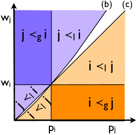
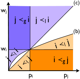
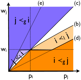
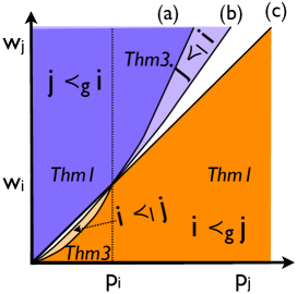
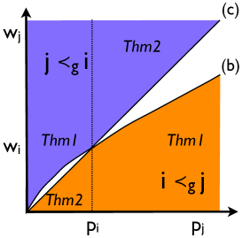
		(a) $w_{j}=w_{i}(p_{j}/p_{i})^{2-\beta}$ (b) $w_{j}=w_{i}\frac{(p_{i}+p_{j})^{\beta}-p_{i}^{\beta}}{(p_{i}+p_{j})^{\beta}-p_{j}^{\beta}}$ (c) $w_{j}=w_{i}p_{j}/p_{i}$ (d) $w_{j}=w_{i}p_{j}/2p_{i}$ (e) $w_{j}=2w_{i}p_{j}/p_{i}$

Figure 1: Illustration of our contribution (bottom row) compared to previous results (top row), using a similar representation as in (Höhn and Jacobs 2012a). Every point in the diagram represents a job $j$ with respect to some fixed job $i$. The space is divided into regions where $i\prec_{\ell}j$ holds or $j\prec_{\ell}i$ or none. These regions contain subregions where we know that the stronger condition $\prec_{g}$ holds. The boundaries are defined by functions which are named from (a) to (e). The last 2 diagrams also indicate the related theorems.

4 Technical lemmas

This section contains several technical lemmas used in the proof of our main theorems.

Lemma 1

For $0<\beta<1,a<b$ and $p_{i}>p_{j}$,

$$\left(\frac{p_{i}}{p_{j}}\right)^{1-\beta}\cdot\frac{f(b+p_{i})-f(a+p_{i})}{f(b+p_{j})-f(a+p_{j})}\geq 1.$$

Proof  For this purpose we define the function

$$g(x):=x^{1-\beta}(f(b+x)-f(a+x))$$

and show that $g$ is increasing, which implies $g(p_{i})/g(p_{j})\geq 1$ as required. So we have to show $g^{\prime}(x)>0$ in other words

$$\phantom{+}(1-\beta)x^{-\beta}\big{(}f(b+x)-f(a+x)\big{)}$$

$$+x^{1-\beta}\big{(}f^{\prime}(b+x)-f^{\prime}(a+x)\big{)} \geq 0$$

$$\Leftrightarrow\phantom{+}(1-\beta)x^{-\beta}\big{(}(b+x)^{\beta}-(a+x)^{\beta}\big{)}$$

$$+x^{1-\beta}\beta\big{(}(b+x)^{\beta-1}-(a+x)^{\beta-1}\big{)} \geq 0$$

$$\Leftrightarrow\phantom{-}(b+x)^{\beta-1}((1-\beta)(b+x)+\beta x)$$

$$-(a+x)^{\beta-1}((1-\beta)(a+x)+\beta x) \geq 0.$$

To establish the last inequality, we introduce another function

$$r(z):=(z+x)^{\beta-1}((1-\beta)(z+x)+\beta x)$$

and show that $r(z)$ is increasing, implying $r(b)\geq r(a)$. By analyzing its derivative we obtain

$$r^{\prime}(z)= \phantom{+}(\beta-1)(z+x)^{\beta-2}((1-\beta)(z+x)+\beta x)$$

$$+(1-\beta)(z+x)^{\beta-1}$$

$$= (z+x)^{\beta-2}(1-\beta)((\beta-1)(z+x)-x\beta+z+x)$$

$$= (z+x)^{\beta-2}(1-\beta)(\beta z),$$

which is positive as required. This concludes the proof. $\Box$

Some of our proofs are based on particular properties which are enumerated in the following lemma.

Lemma 2

The function $f(t)=t^{\beta}$ defined for $\beta\geq 1$ satisfies the following properties.

1. $f(x)\geq 0$ for $x\geq 0$.

2. $f$ is convex and non-decreasing, i.e. $f^{\prime},f^{\prime\prime}\geq 0$.

3. $f^{\prime}$ is log-concave (i.e. $\log(f^{\prime})$ is concave), which implies that $f^{\prime\prime}/f^{\prime}$ is non-increasing. Intuitively this means that $f$ does not increase much faster than $e^{x}$.

4. For every $b>0$, the function $g_{b}(x)=f(b+e^{x})-f(b)$ is log-convex in $x$. Intuitively this means that $f(b+e^{x})-f(b)$ increases faster than $e^{cx}$ for some $c>0$. Formally this means

   $$yf^{\prime}(b+y)/\big{(}f(b+y)-f(b)\big{)}$$ (1)

   is increasing in $y$.

The proof is based on standard functional analysis and is omitted.

Lemma 3

For $a<b$, the fraction

$$\frac{f^{\prime}(b)-f^{\prime}(a)}{f(b)-f(a)}$$

• is decreasing in $a$ and decreasing in $b$ for any $\beta>1$

• and is increasing in $a$ and increasing in $b$ for any $0<\beta<1$.

Proof  First we consider the case $\beta>1$. We can write $f^{\prime}(b)-f^{\prime}(a)=\int_{a}^{b}f^{\prime\prime}(x)dx$ and $f(b)-f(a)=\int_{a}^{b}f^{\prime}(x)dx$. Note that $f^{\prime\prime}$ and $f^{\prime}$ are non-negative. By $\beta>1$ and Lemma 2 $f^{\prime}$ is log-concave, which means that $f^{\prime\prime}(x)/f^{\prime}(x)$ is non-increasing in $x$. This implies

$$\int_{a}^{b}\frac{f^{\prime\prime}(b)}{f^{\prime}(b)}f^{\prime}(x)dx \leq\int_{a}^{b}\frac{f^{\prime\prime}(x)}{f^{\prime}(x)}f^{\prime}(x)dx$$

$$\leq\int_{a}^{b}\frac{f^{\prime\prime}(a)}{f^{\prime}(a)}f^{\prime}(x)dx$$

Hence

$$\frac{\int_{a}^{b}f^{\prime\prime}(b)dx}{\int_{a}^{b}f^{\prime}(b)dx}\leq\frac{\int_{a}^{b}f^{\prime\prime}(x)dx}{\int_{a}^{b}f^{\prime}(x)dx}\leq\frac{\int_{a}^{b}f^{\prime\prime}(a)dx}{\int_{a}^{b}f^{\prime}(a)dx}.$$

For positive values $u_{1},u_{2},u_{3},v_{1},v_{2},v_{3}$ with $u_{1}/v_{1}\leq u_{2}/v_{2}\leq u_{3}/v_{3}$ we have

$$\frac{u_{1}+u_{2}}{v_{1}+v_{2}}\leq\frac{u_{2}}{v_{2}}\leq\frac{u_{2}+u_{3}}{v_{2}+v_{3}}.$$

We use this property for $a^{\prime}<a<b<b^{\prime}$

$$\frac{u_{1}}{v_{1}} =\frac{\int_{b}^{b^{\prime}}f^{\prime\prime}(x)dx}{\int_{b}^{b^{\prime}}f^{\prime}(x)dx},$$

$$\frac{u_{2}}{v_{2}} =\frac{\int_{a}^{b}f^{\prime\prime}(x)dx}{\int_{a}^{b}f^{\prime}(x)dx},$$

$$\frac{u_{3}}{v_{3}} =\frac{\int_{a^{\prime}}^{a}f^{\prime\prime}(x)dx}{\int_{a^{\prime}}^{a}f^{\prime}(x)dx}$$

and obtain

$$\frac{\int_{a^{\prime}}^{b}f^{\prime\prime}(x)dx}{\int_{a^{\prime}}^{b}f^{\prime}(x)dx}\leq\frac{\int_{a}^{b}f^{\prime\prime}(x)dx}{\int_{a}^{b}f^{\prime}(x)dx}\leq\frac{\int_{a}^{b^{\prime}}f^{\prime\prime}(x)dx}{\int_{a}^{b^{\prime}}f^{\prime}(x)dx}.$$

For the case $0<\beta<1$ the argument is the same using the fact that $f^{\prime\prime}(x)/f^{\prime}(x)$ is non-decreasing in $x$. $\Box$

The previous lemma permits to show the following corollary.

Corollary 1

For $t\geq 0$ let the function $q$ be defined as

$$q(t):=\frac{f(t+p_{j})-f(t)}{f(t+p_{i})-f(t)}.$$

For $p_{i}>p_{j}$, if $\beta>1$ then $q$ is increasing and if $0<\beta<1$ then $q$ is decreasing.

Proof  We only prove the case $\beta>1$, the other case is similar. Showing that $q(t)$ is increasing, it suffices to show that

$$\ln q(t)=\ln(f(t+p_{j})-f(t))-\ln(f(t+p_{i})-f(t))$$

is increasing. To this purpose we notice that the derivative

$$\frac{f^{\prime}(t+p_{j})-f^{\prime}(t))}{f(t+p_{j})-f(t))}-\frac{f^{\prime}(t+p_{i})-f^{\prime}(t))}{f(t+p_{j})-f(t))}$$

is positive by Lemma 1 and $p_{i}>p_{j}$. $\Box$

Lemma 4

If $\beta>1,a<b$ and

$$g(x)=x\frac{f(b+x)-f(x+a)}{f(b+x)-f(b)},$$

then $g(x)$ is a non-decreasing function of $x$.

Proof  Equivalently, we show that $\ln g(x)=\ln(x)+\ln\big{(}f(b+x)-f(a+x)\big{)}-\ln\big{(}f(b+x)-f(b)\big{)}$ is non-decreasing. Taking derivative of the right hand side, we show

$$\frac{1}{x}+\frac{f^{\prime}(b+x)-f^{\prime}(a+x)}{f(b+x)-f(a+x)}-\frac{f^{\prime}(b+x)}{f(b+x)-f(b)}\geq 0.$$

By log-concavity of $f^{\prime}$ and Lemma 3, the second term is minimized when $a$ approaches $b$, and hence is at least $f^{\prime\prime}(b+x)/f^{\prime}(b+x)$. Therefore it is enough to show that

$$\frac{1}{x}+\frac{f^{\prime\prime}(b+x)}{f^{\prime}(b+x)}-\frac{f^{\prime}(b+x)}{f(b+x)-f(b)}\geq 0,$$

which is equivalent in showing that

$$\ln(x)+\ln(f^{\prime}(b+x))-\ln\big{(}f(b+x)-f(b)\big{)}$$

is non-decreasing $x$. The later derives from the fact that $xf^{\prime}(b+x)/\big{(}f(b+x)-f(b)\big{)}$ is non-decreasing, which follows from assumption in (1).$\Box$

5 Characterization of the local order property

To simplify notation, throughout the paper we assume that no two jobs have the same processing time, weight or Smith-ratio (weight over processing time). The proofs extend to the general case by considering an additional tie-breaking rule between jobs with identical parameters. For convenience we extend the notation of the penalty function $f$ to the makespan of schedule $S$ as $f(S):=f(\sum_{i\in S}p_{i})$. Also we denote by $F(S)$ the cost of schedule $S$.

In order to analyze the effect of exchanging adjacent jobs, we define the following function on $t\geq 0$

$$\phi_{ij}(t):=\frac{f(t+p_{i}+p_{j})-f(t+p_{j})}{f(t+p_{i}+p_{j})-f(t+p_{i})}.$$

Note that $\phi_{ij}(t)$ is well defined since $f$ is strictly increasing by assumption and the durations $p_{i},p_{j}$ are non-zero. This function $\phi_{ij}$ permits us to analyze algebraically the local order property, since

$$i\prec_{\ell}j\>\Leftrightarrow\>\forall t\geq 0:\phi_{ij}(t)<\frac{w_{i}}{w_{j}}.$$ (2)

The following technical lemmas show properties of $\phi_{ij}$ and relate them to properties of $f$.

Lemma 5

If $p_{i}\neq p_{j}$ then $\phi_{ij}$ is strictly monotone, in particular:

• If $p_{i}>p_{j}$ and $\beta>1$, then $\phi_{ij}$ is strictly increasing.

• If $p_{i}<p_{j}$ and $\beta>1$, then $\phi_{ij}$ is strictly decreasing.

• If $p_{i}>p_{j}$ and $\beta<1$, then $\phi_{ij}$ is strictly decreasing.

• If $p_{i}<p_{j}$ and $\beta<1$, then $\phi_{ij}$ is strictly increasing.

Proof  We only show this statement for the first case $p_{i}>p_{j}$ and $\beta>1$, and the other cases are similar. In order to show that $\phi_{ij}$ is strictly increasing we prove that $\ln\phi_{ij}$ is increasing. For this we analyze its derivative which is

$$\frac{f^{\prime}(t+p_{i}+p_{j})-f^{\prime}(t+p_{j})}{f(t+p_{i}+p_{j})-f(t+p_{j})}-\frac{f^{\prime}(t+p_{i}+p_{j})-f^{\prime}(t+p_{i})}{f(t+p_{i}+p_{j})-f(t+p_{i})}.$$

The derivative is positive by Lemma 3. $\Box$

Figure 2: Examples of the function $\phi_{ij}(t)$ for $\beta=0.5$ and $\beta=2$, as well as for the cases $p_{i}>p_{j}$ and $p_{i}<p_{j}$.

Lemma 6

For any jobs $i,j$, we have $\lim_{t\rightarrow\infty}\phi_{ij}(t)=p_{i}/p_{j}.$

Proof  By the mean value Theorem, for any differentiable function $f$ and $y,x$ it holds that $f(y)=f(x)+(y-x)f^{\prime}(\eta)$ for some $\eta\in[x,y]$. Thus $(t+p_{i}+p_{j})^{\beta}-(t+p_{i})^{\beta}=\beta p_{j}(t+p_{i}+\eta)^{\beta-1}$ for some $\eta\in[0,p_{j}]$ and $(t+p_{i}+p_{j})^{\beta}-(t+p_{j})^{\beta}=\beta p_{i}(t+p_{j}+\gamma)^{\beta-1}$ for some $\gamma\in[0,p_{i}]$. Moreover, for any $\beta>0$ and $a>0$, $\lim_{t\rightarrow\infty}(t+a)^{\beta-1}/t^{\beta-1}=1$. Therefore,

$$\lim_{t\rightarrow\infty}\phi_{ij}(t)=\lim_{t\rightarrow\infty}\frac{(t+p_{i}+p_{j})^{\beta}-(t+p_{j})^{\beta}}{(t+p_{i}+p_{j})^{\beta}-(t+p_{i})^{\beta}}=\frac{p_{i}}{p_{j}}.$$

$\Box$

These two lemmas permit to characterize the local order property, see Figure 1.

Lemma 7

For any two jobs $i,j$ we have $i\prec_{\ell}j$ if and only if

• $\beta>1$ and $p_{i}\leq p_{j}$ and $w_{j}/w_{i}\leq\phi_{ji}(0)$ or

• $\beta>1$ and $p_{i}\geq p_{j}$ and $w_{j}/w_{i}\leq p_{j}/p_{i}$ or

• $0<\beta<1$ and $p_{i}\leq p_{j}$ and $w_{j}/w_{i}\leq p_{j}/p_{i}$ or

• $0<\beta<1$ and $p_{i}\geq p_{j}$ and $w_{j}/w_{i}\leq\phi_{ji}(0)$.

6 The global order property

In this section we characterize the global order property of two jobs $i,j$ in the convex case $\beta>1$, and provide sufficient conditions on the concave case $0\leq\beta<1$. Our contributions are summarized graphically in Figure 1.

6.1 Global order property for $p_{i}\leq p_{j}$

In this section we give the proof of the conjecture in case $i$ has processing time not larger than $j$. Intuitively this seems the easier case, as exchanging $i$ with $j$ in the schedule $AjBi$ makes jobs from $B$ complete earlier. However the benefit of the exchange on these jobs cannot simply be ignored in the proof. A simple example with $\beta=2$ shows why this is so. Let $i,j,k$ be 3 jobs with $p_{i}=4,w_{i}=1,p_{j}=8,w_{j}=1.5,p_{k}=1,w_{k}=0$. Then $i\prec_{\ell}j$, but exchanging $i,j$ in the schedule $jki$ increases the objective value, as $F(ikj)=4^{2}+1.5\cdot 13^{2}=269.5$ while $F(jki)=1.5\cdot 8^{2}+13^{2}=265$. Now if we raise $w_{k}$ to $0.3$, then we obtain an interesting instance. It satisfies $F(jki)<F(jik)$ and $jki$ is the optimal schedule, but it cannot be shown with an exchange argument from $ikj$ without taking into account the gain on job $k$ during the exchange.

Theorem 1

The implication $i\prec_{\ell}j\Rightarrow i\prec_{g}j$ holds when $p_{i}\leq p_{j}$.

Proof  The proof holds in fact for any increasing penalty function $f$. Let $A,B$ be two arbitrary job sequences. We will show that the schedule $AjBi$ has strictly higher cost than one of the schedules $AijB,AiBj$.

First if $F(AjBi)\geq F(AjiB)$, then by $i\prec_{\ell}j$ we have even $F(AjBi)>F(AijB)$. So for the remaining case we assume $F(AjBi)<F(AjiB)$ and will show $F(AjBi)>F(AiBj)$. By $i\prec_{\ell}j$ it would be enough to show the even stronger inequality

$$F(AjiB)-F(AijB) <F(AjBi)-F(AiBj),$$

or equivalently

$$F(AjiB)-F(AjBi) <F(AijB)-F(AiBj).$$

The left hand side is positive by assumption, so it would be enough to show

$$\min_{t}\phi_{ji}(t) \left(F(AjiB)-F(AjBi)\right)$$

$$< ~{}F(AijB)-F(AiBj),$$ (3)

since $\phi_{ji}(t)>1$ by $p_{i}<p_{j}$.

We introduce the following notation. Denote the jobs in $B$ by $1,\ldots,k$ and for every job $1\leq h\leq k$ denote by $l_{h}$ the total processing time of all jobs from $1$ to $h$. We show the inequality, by analyzing separately the contribution of jobs $h\in B$, and of the jobs $i,j$. By definition of $\phi_{ji}$ we have

$$\phi_{ji}(l_{h})\left(f(p_{i}+p_{j}+l_{h})-f(p_{j}+l_{h})\right)$$

$$= f(p_{i}+p_{j}+l_{h})-f(p_{i}+l_{h}),$$

which implies

$$\min_{t}\phi_{ji}(t)w_{h}\left(f(p_{i}+p_{j}+l_{h})-f(p_{j}+l_{h})\right)$$

$$\leq w_{h}\left(f(p_{i}+p_{j}+l_{h})-f(p_{i}+l_{h})\right).$$ (4)

To analyze the contribution of jobs $i,j$ we observe that by $i\prec_{\ell}j$ we have $w_{j}<\min\phi_{ji}w_{i}$ which implies

$$\min_{t}\phi_{ji}(t)w_{i}\left(f(a+p_{i}+p_{j})-f(a+p_{i}+p_{j}+l_{k})\right)$$

$$< w_{j}\left(f(a+p_{i}+p_{j})-f(a+p_{i}+p_{j}+l_{k})\right).$$ (5)

Summing up (4) for every $1\leq h\leq k$ and (5) yields (3) as required, and completes the proof. $\Box$

6.2 Global order property for $\beta>1$

Theorem 2

The implication $i\prec_{\ell}j\Rightarrow i\prec_{g}j$ holds when $\beta\geq 1$.

Proof  By Theorem 1 it suffices to consider the case $p_{j}<p_{i}$. Assume $i\prec_{\ell}j$ and consider a schedule $S$ of the form $AjBi$ for some job sequences $A,B$.

The proof is by induction on the number of jobs in $B$. The base case $B=\emptyset$ follows from $i\prec_{\ell}j$. For the induction step, we assume that $A^{\prime}jB^{\prime}i$ is suboptimal for all job sequences $A^{\prime},B^{\prime}$ where $B^{\prime}$ has strictly less jobs than $B$. Formally we denote $B$ as the job sequence $1,2,\ldots,k$ for some $k\geq 1$. If for some $1\leq h\leq k$ we have

$$F(AjBi)\geq F(A(12\ldots h)j(h+1,\ldots,k)i),$$

then by induction we immediately obtain that $AjBi$ is suboptimal. Therefore we assume

$$\forall 1\leq h\leq k:F(AjBi)<F(A(12\ldots h)j(h+1,\ldots,k)i).$$ (6)

Then we show that $F(AjBi)>F(AiBj)$ to establish sub-optimality of $AjBi$.

For the remainder of the proof, we introduce the following notations. We denote by $a$ the total processing time of $A$. In addition we use $h$ and $h^{\prime}$ to index the jobs in $B$, and denote by $l_{h}$ the total processing time of jobs $1,2,\ldots,h$, and by $b=a+l_{k}$ the total processing time of $AB$. We also introduce the expressions

$$\delta^{i}_{h}:=f(a+p_{i}+l_{h})-f(a+l_{h})$$

and

$$\gamma^{i}_{h}:=f(a+p_{i}+l_{h})-f(a+p_{i}+l_{h-1})$$

and define $\delta^{j}_{h},\gamma^{j}_{h}$ analogously.

Equations (6) imply that

$$\sum_{h^{\prime}=1}^{h}w_{h^{\prime}}\big{(}f(a+p_{j}+l_{h^{\prime}})-f(a+l_{h^{\prime}})\big{)}$$

$$\leq w_{j}\big{(}f(a+p_{j}+l_{h})-f(a+p_{j})\big{)}$$

$$= w_{j}\sum_{h^{\prime}=1}^{h}\big{(}f(a+p_{j}+l_{h^{\prime}})-f(a+p_{j}+l_{h^{\prime}-1})\big{)}$$ (7)

where we use the convention that $l_{0}=0$.

We restate (7) as follows: For each $1\leq h\leq k$,

$$w_{1}\delta^{j}_{1}+\ldots+w_{h}\delta^{j}_{h}\leq w_{j}(\gamma^{j}_{1}+\ldots+\gamma^{j}_{h})$$ (8)

For $a<b$ define

$$g(x)=x\frac{f(b+x)-f(x+a)}{f(b+x)-f(b)}.$$

By Lemma 4 $g$ is non-decreasing in $x$.

We need to show that $F(AiBj)<F(AjBi)$. As $p_{i}>p_{j}$ by case assumption, when we move from $AjBi$ to $AiBj$, the completion times of $j$ and the jobs in $B$ increase and that of $i$ decreases. Thus the statement is equivalent to showing that

$$\sum_{h=1}^{k}w_{h}\biggl{(}f(a+p_{i}+l_{h})-f(a+p_{j}+l_{h})\biggl{)}$$

$$< \phantom{-}w_{i}\big{(}f(a+p_{j}+p_{i}+l_{k})-f(a+p_{i})\big{)}$$

$$-w_{j}\big{(}f(a+p_{j}+p_{i}+l_{k})-f(a+p_{j})\big{)}$$ (9)

Now, by assumption $i\prec_{\ell}j$, it holds that

$$w_{j}\big{(}f(a+p_{j}+p_{i}+l_{k})-f(a+p_{j}+l_{k})\big{)}$$

$$< w_{i}\big{(}f(a+p_{i}+p_{j}+l_{k})-f(a+p_{i}+l_{k})\big{)},$$

thus to show (6.2) it suffices to show that

$$\sum_{h=1}^{k}w_{h}\big{(}f(a+p_{i}+l_{h})-f(a+p_{j}+l_{h})\big{)}$$

$$\leq \phantom{-}w_{i}\big{(}f(a+p_{i}+l_{k})-f(a+p_{i})\big{)}$$

$$-w_{j}\big{(}f(a+p_{j}+l_{k})-f(a+p_{j})\big{)}.$$ (10)

We reformulate (10) as

$$\sum_{h=1}^{k}w_{h}(\delta^{i}_{h}-\delta^{j}_{h})\leq w_{i}\sum_{h=1}^{k}\gamma^{i}_{h}-w_{j}\sum_{h}\gamma^{j}_{h}.$$

Since $w_{i}\geq w_{j}p_{i}/p_{j}$ by Lemma 7, it suffices to show that for every $1\leq h\leq k$,

$$\sum_{h=1}^{k}w_{h}(\delta^{i}_{h}-\delta^{j}_{h})\leq w_{j}\sum_{h=1}^{k}\biggl{(}\frac{p_{i}}{p_{j}}\gamma^{i}_{h}-\gamma^{j}_{h}\biggr{)}.$$ (11)

We define for every job $1\leq h\leq k$

$$q_{h}:=\frac{\delta^{i}_{h}}{\delta^{j}_{h}}-\frac{\delta^{i}_{h+1}}{\delta^{j}_{h+1}}$$

where we use the convention $\delta^{i}_{k+1}/\delta^{j}_{k+1}=1$. Note that by Corollary 1, all $q_{h}$ are non-negative.

Multiplying for a given $h$, equation (8) by $q_{h}$, and summing over all $1\leq h\leq k$ we obtain

$$\sum_{h=1}^{k}w_{h}\delta^{j}_{h}(\sum_{h^{\prime}\geq h}q_{h^{\prime}})\leq w_{j}\sum_{h=1}^{k}\gamma^{j}_{h}(\sum_{h^{\prime}\geq h}q_{h^{\prime}}).$$

As the sum over $q_{h^{\prime}}$ telescopes, we can rewrite the above as

$$\sum_{h=1}^{k}w_{h}(\delta^{i}_{h}-\delta^{j}_{h})\leq w_{j}\sum_{h=1}^{k}\gamma^{j}_{h}(\delta^{i}_{h}/\delta^{j}_{h}-1)$$

Thus to prove (11), it suffices to show that

$$\gamma^{j}_{h}(\delta^{i}_{h}/\delta^{j}_{h}-1)\leq(p_{i}/p_{j})\gamma^{i}_{h}-\gamma^{j}_{h}$$

or equivalently,

$$\delta^{i}_{h}/\delta^{j}_{h}\leq(p_{i}/p_{j})(\gamma^{i}_{h}/\gamma^{j}_{h})$$

But this is exactly what Lemma 4 gives us. In particular,

$$\gamma^{j}_{h}/\delta^{j}_{h}p_{j}\leq p_{i}\gamma^{i}_{h}/\delta^{i}_{h}$$

is equivalent to

$$p_{j}\frac{f(a+p_{j}+l_{h})-f(a+p_{j}+l_{h-1})}{f(a+p_{j}+l_{h})-f(a+l_{h})}$$

$$\leq p_{i}\frac{f(a+p_{i}+l_{h})-f(a+p_{i}+l_{h-1})}{f(a+p_{i}+l_{h})-f(a+l_{h})}$$

which follows Lemma 4 since $p_{i}\geq p_{j}$. Therefore, the theorem holds. $\Box$

6.3 Global order property for $0<\beta<1$ and $p_{j}\leq p_{i}$

Theorem 3

The implication $i\prec_{\ell}j\Rightarrow i\prec_{g}j$ holds when $p_{j}\leq p_{i}$, $w_{i}/w_{j}\geq(p_{i}/p_{j})^{2-\beta}$ and $0<\beta<1$.

Proof  The proof is along the same lines as the previous one. Hence we assume (6) and need to show $F(AjBi)>F(AiBj)$, and for this purpose show

$$F(ABji)-F(ABij)<F(AjBi)-F(AiBj),$$

where the left hand side is positive by $i\prec_{\ell}j$. Equivalently we have to show

$$F(ABji)-F(AjBi)<F(ABij)-F(AiBj).$$ (12)

First we claim that

$$\frac{w_{i}}{w_{j}}>\left(\frac{p_{i}}{p_{j}}\right)^{1-\beta}.$$ (13)

Indeed, from Lemma 7 we have $w_{j}/w_{i}\leq\phi_{ji}(0)$. By Lemma 5, the function $\phi_{ji}(t)$ is increasing, and by Lemma  6, it is upper bounded by $p_{j}/p_{i}$. Hence $w_{j}/w_{i}\leq p_{j}/p_{i}$, and for $0<\beta<1$ and $p_{j}\leq p_{i}$ inequality (13) follows.

Therefore by Lemma 1 we have

$$\frac{w_{i}}{w_{j}}\frac{f(b+p_{i})-f(a+p_{i})}{f(b+p_{j})-f(a+p_{j})} >$$

$$\left(\frac{p_{i}}{p_{j}}\right)^{1-\beta}\frac{f(b+p_{i})-f(a+p_{i})}{f(b+p_{j})-f(a+p_{j})} \geq 1.$$ (14)

For convenience we denote

$$\Delta(t):=\sum_{h\in B}w_{h}(f(a+l_{h}+t)-f(a+l_{h})).$$

We have

$$0< F(ABji)-F(AjBi)$$

$$= w_{j}(f(b+p_{j})-f(a+p_{j}))-\Delta(p_{j})$$

$$< \phantom{\cdot}\frac{w_{i}}{w_{j}}\frac{f(b+p_{i})-f(a+p_{i})}{f(b+p_{j})-f(a+p_{j})}\cdot$$

$$\cdot\big{(}w_{j}(f(b+p_{j})-f(a+p_{j}))-\Delta(p_{j})\big{)}$$

$$= \phantom{-}w_{i}\big{(}f(b+p_{i})-f(a+p_{i})\big{)}$$

$$-\frac{w_{i}}{w_{j}}\frac{f(b+p_{i})-f(a+p_{i})}{f(b+p_{j})-f(a+p_{j})}\Delta(p_{j})$$

$$< w_{i}\big{(}f(b+p_{i})-f(a+p_{i})\big{)}$$

$$-\frac{w_{i}}{w_{j}}\frac{f(b+p_{i})-f(a+p_{i})}{f(b+p_{j})-f(a+p_{j})}\min_{t\geq 0}\frac{f(t+p_{j})-f(t)}{f(t+p_{i})-f(t)}\Delta(p_{i}).$$

The first inequality follows from assumption (6) with $h=k$. The second inequality follows from (14). The third inequality holds since $f(t+p_{j})<f(t+p_{i})$ for all $t\geq 0$.

In order to upper bound the latter expression by

$$w_{i}(f(b+p_{i})-f(a+p_{i}))-\Delta(p_{i})$$

$$= F(ABij)-F(AiBj)$$

as required, it suffices to show

$$\frac{w_{i}}{w_{j}}\frac{f(b+p_{i})-f(a+p_{i})}{f(b+p_{j})-f(a+p_{j})}\min_{t\geq 0}\frac{f(t+p_{j})-f(t)}{f(t+p_{i})-f(t)}\geq 1.$$

By $0<\beta<1$ and Corollary 1 the fraction $\frac{f(t+p_{j})-f(t)}{f(t+p_{i})-f(t)}$ is decreasing, and its limit when $t\rightarrow\infty$ is $p_{j}/p_{i}$, by the same analysis as in the proof of Lemma 6. Therefore $\min_{t\geq 0}\frac{f(t+p_{j})-f(t)}{f(t+p_{i})-f(t)}\geq\frac{p_{j}}{p_{i}}$. Hence

$$\frac{w_{i}}{w_{j}}\frac{f(b+p_{i})-f(a+p_{i})}{f(b+p_{j})-f(a+p_{j})}\min_{t\geq 0}\frac{f(t+p_{j})-f(t)}{f(t+p_{i})-f(t)}$$

$$\geq \frac{w_{i}}{w_{j}}\frac{f(b+p_{i})-f(a+p_{i})}{f(b+p_{j})-f(a+p_{j})}\frac{p_{j}}{p_{i}}$$

$$\geq \left(\frac{p_{i}}{p_{j}}\right)^{2-\beta}\frac{f(b+p_{i})-f(a+p_{i})}{f(b+p_{j})-f(a+p_{j})}\frac{p_{j}}{p_{i}}$$

$$= \left(\frac{p_{i}}{p_{j}}\right)^{1-\beta}\frac{f(b+p_{i})-f(a+p_{i})}{f(b+p_{j})-f(a+p_{j})}\geq 1.$$

where the second inequality follows from the theorem hypothesis and the last inequality from Lemma 1. This concludes the proof of the theorem. $\Box$

7 Generalization

We can provide some technical generalizations of the aforementioned theorems. For any pair of jobs $i,j$, and job sequence $T$ of total length $t$, we denote by $i\prec_{\ell(t)}j$ the property $F(Tij)<F(Tji)$. Now suppose that none of $i\prec_{\ell}j$ or $j\prec_{\ell}j$ holds, and say $p_{i}>p_{j}$ and $\beta>1$. Then from Lemma 5 it follows that there exist a unique time $t$, such that for all $t^{\prime}<t$ we have $i\prec_{\ell(t^{\prime})}j$ and for all $t^{\prime}>t$ we have $j\prec_{\ell(t^{\prime})}i$. These properties are denoted respectively by $i\prec_{\ell[0,t)}j$ and $j\prec_{\ell(t,\infty)}j$. In case $p_{i}<p_{j},\beta>1$ or $p_{i}>p_{j},0<\beta<1$, we have the symmetric situation $j\prec_{\ell[0,t)}i$ and $i\prec_{\ell(t,\infty)}j$.

This notation can be extended also to the global order property. If for every job sequences $A,B$ with $A$ having total length at least $t$ we have $F(AiBj)<F(AjBi)$, then we say that $i,j$ satisfy the global order property in the interval $(t,\infty)$ and denote it by $i\prec_{g(t,\infty)}j$. The property $i\prec_{g[0,t)}j$ is defined similarly for job sequences $A,B$ of total length at most $t$.

The proof of Theorem 2 actually shows the stronger statement: if $\beta>1$ and $p_{i}\geq p_{j}$, then $j\prec_{\ell(t,\infty)}i$ implies $j\prec_{g(t,\infty)}i$. The same implication does not hold for interval $[0,t)$, as shown by the following counter example. It consists of a 3-job instance for $\beta=2$ with $p_{i}=13,w_{i}=7,p_{j}=8,w_{j}=5,p_{k}=1,w_{k}=1$. For $t=19/18$, we have $i\prec_{\ell[0,t)}j$ and $j\prec_{\ell(t,\infty)}i$. But the unique optimal solution is the sequence $jki$, meaning that we do not have $i\prec_{g[0,t)}j$.

These generalizations can be summarized as follows.

	$p_{i}\leq p_{j}$	$p_{i}\geq p_{j}$
	$0<\beta<1$	$\beta>1$
$i\prec_{\ell[0,t)}j\Rightarrow i\prec_{g[0,t)}j$	Yes	No
$j\prec_{\ell(t,\infty)}i\Rightarrow j\prec_{g(t,\infty)}i$	Open	Yes

8 Experimental study

We conclude this paper with an experimental study, evaluating the impact of the proposed rules on the performance of a search procedure. The experiments are based on a C++ program executed on a GNU/Linux machine with 3 Intel Xeon processors, each with 4 cores, running at 2.6Ghz and 32Gb RAM. In order to be independent on the machine environment, we measured the number of generated search nodes rather than running time. Hence we use a timeout which is not expressed in seconds, but in time units corresponding to the processing of a search node by the program. Note that we use the rules that we have proved (not the ones in the conjecture). Following the approach described in (Höhn and Jacobs 2012a), we consider the Algorithm A* by Hart et al (1972).

The search space is the directed acyclic graph consisting of all subsets $S\subseteq\{1,\ldots,n\}$. Note that the potential search space has size $2^{n}$ which is already less than the space of the $n!$ different schedules. In this graph for every vertex $S$ there is an arc to $S\backslash\{j\}$ for any $j\in S$. It is labeled with $j$, and has cost $w_{j}t^{\beta}$ for $t=\sum_{i\in S}p_{i}$. Every directed path from the root $\{1,\ldots,n\}$ to the target $\{\}$ corresponds to a schedule of an objective value being the total arc cost.

The algorithm A* finds a shortest path from the root to the target vertex, and as Dijkstra’s algorithm uses a priority queue to select the next vertex to explore. But the difference of A* is that it uses as weight for vertex $u$ not only the distance from the source to $u$, but also a lower bound on the distance from $u$ to the destination. A set $S$ is maintained containing all vertices $u$ for which a shortest path has already been discovered. Initially $S=\{s\}$ for the root vertex $s$. In Dijkstra’s algorithm the priority queue contains all remaining vertices $v$, with the priority $\min_{u\in S}d(s,u)+w(u,v)$, where $w(u,v)$ is the weight of the arc $(u,v)$. However in the algorithm A* this priority is replaced by $\min_{u\in S}d(s,u)+w(u,v)+h(v)$, where $h$ is some lower bound on the distance from $v$ to the target. This function should satisfy $h(v)=0$ if $v$ is the target and $h(u)\leq w(u,v)+h(v)$ for every arc $(u,v)$. The function $h$ used in our experiments satisfies these properties.

Pruning is done when constructing the list of outgoing arcs at some vertex $S$. Potentially every job $j\in S$ can generate an arc, but order properties might prevent that. Let $i$ be the label of the arc leading to $S$ (assuming $S$ is not the root). Let $t_{1}=\sum_{k\in S}p_{k}$. We distinguish two kind of pruning rules:

Arc pruning.

The arc from $S$ to $S\setminus\{j\}$ for $j\in S$ is pruned if $i\prec_{\ell(t_{1}-p_{j})}j$, because placing job $j$ adjacent to $i$ at this position would be suboptimal.

Vertex pruning.

All arcs leaving vertex $S$ are pruned, if there is a job $j\in S$ with $i\prec_{g[0,t_{1}]}j$, as again placing job $j$ somewhere before job $i$ would be suboptimal.

In the lack of a complete characterization of the global precedence relation, we have to weaken the vertex pruning rule by replacing $i\prec_{g[0,t_{1}]}j$ with a condition implying $i\prec_{g}j$. These would be the Sen-Dileepan-Ruparel condition in general or for $\beta=2$ the Mondal-Sen-Höhn-Jacobs conditions. Our pruning rules consist of using our conditions for global precedence.

In a search tree such an arc pruning would cut the whole subtree attached to that arc, but in a directed acyclic graph (DAG) the improvement is not so significant. As the typical in-degree of a vertex is linear in $n$, a linear number of arc-cut is necessary to remove a vertex from the DAG.

Figure 3 illustrates the DAG explored by A* for $\beta=2$ on the instance consisting of the following (processing time, priority weight) pairs :

$$(10,5),(10,5),(11,3),(13,6),(8,4),(12,6).$$

Arcs are labeled with their cost. The last two arcs have the same weight, as the lower bound on single job sets is tight.

Figure 3: Example of the portion of the search graph explored by the algorithm A*.

A simple additional pruning could be done when remaining jobs to be scheduled form a trivial subinstance. By this we mean that all pairs of jobs $i,j$ from this subinstance are comparable with the order $\prec_{\ell[0,t_{1}]}$. In that case the local order is actually a total order, which describes in a simple manner the optimal schedule for this subinstance. In that case we could simply generate a single path from the node $S$ to the target vertex $\{\}$. However experiments showed that detecting this situation is too costly compared with the benefit we could gain from this pruning rule.

8.1 Random instances

We adopt the model of random instances described by Höhn and Jacobs. Most previous experimental results were made by generating processing times and weights uniformly from some interval, which leads to easy instances, since any job pair $i,j$ satisfies with probability $1/2$ the Sen-Dileepan-Ruparel condition, i.e.  $i\prec_{g}j$ or $j\prec_{g}i$. As an alternative, Höhn and Jacobs (2012a) proposed a random model, where the Smith-ratio of a job is selected according to $2^{N(0,\sigma^{2})}$ with $N$ being the normal distribution centered at $0$ with variance $\sigma$. Therefore for $\beta=2$ the probability that two jobs satisfy the Mondal-Sen-Höhn-Jacobs-2 condition depends on $\sigma$, as it compares the Smith-ratio among the jobs.

We adopted their model for other values of $\beta$ as follows. When $\beta>1$, the condition for $i\prec_{g}j$ of our conditions can be approximated, when $p_{j}/p_{i}$ tends to infinity, by the relation $w_{i}/p_{i}\geq\beta w_{j}/p_{j}$. Therefore in order to obtain a similar “hardness” of the random instances for the same parameter $\sigma$ for different values of $\beta>1$, we choose the Smith-ratio according to $2^{N(0,\beta^{2}\sigma^{2})}$. This way the ratio between the Smith-ratios of two jobs is a random variable from the distribution $2^{2N(0,\beta^{2}\sigma^{2})}$, and the probability that this value is at least $\beta$ depends only on $\sigma$.

However when $\beta$ is between $0$ and $1$, the our condition for $i\prec_{g}j$ of our rule can be approximated when $p_{j}/p_{i}$ tends to infinity by the relation $w_{i}/p_{i}\geq 2w_{j}/p_{j}$, and therefore we choose the Smith-ratio of the jobs according to the $\beta$-independent distribution $2^{N(0,4\sigma^{2})}$.

The instances of our main test sets are generated as follows. For each choice of $\sigma\in\{0.1,0.2,\ldots,1\}$ and $\beta\in\{0.5,0.8,1.1,\ldots,3.2\}$, we generated $25$ instances of $20$ jobs each. The processing time of every job is uniformly generated in $\{1,2,\ldots,100\}$. Then the weight is generated according to the above described distribution. Note that the problem is independent from scaling of processing time or weights, motivating the arbitrary choice of the constant $100$.

8.2 Hardness of instances

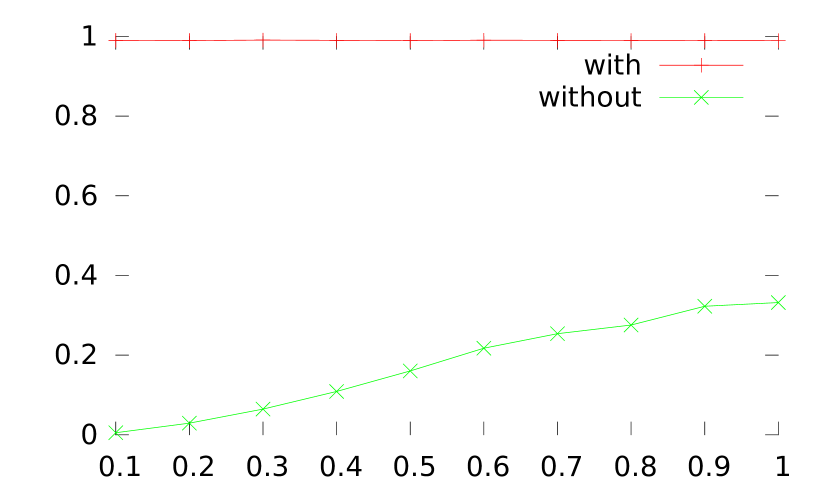
$\beta=0.5$		$\beta=2.0$
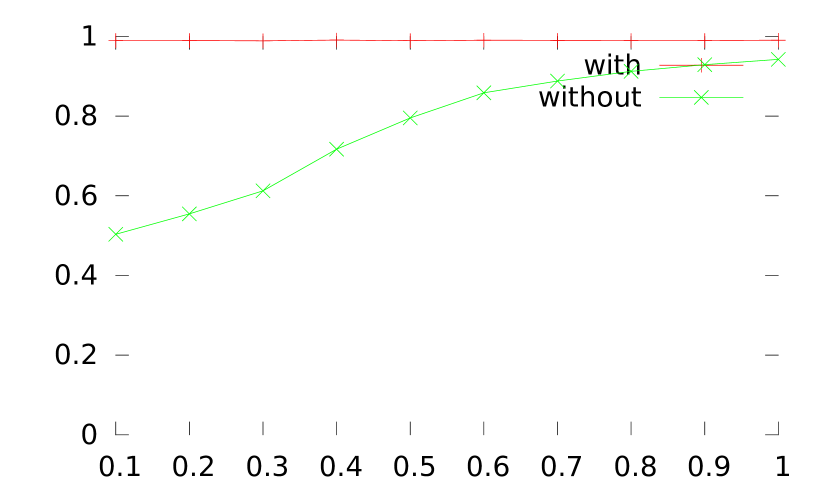
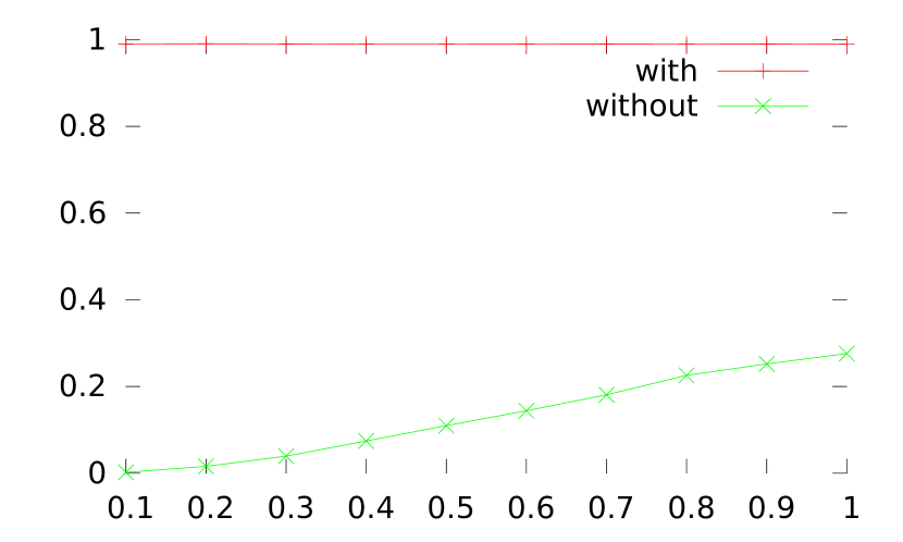
$\beta=0.8$		$\beta=2.3$
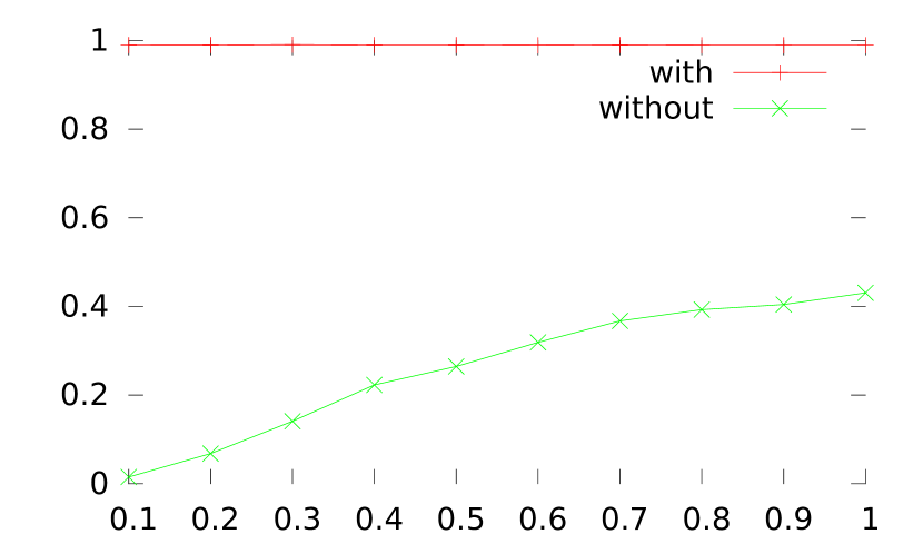
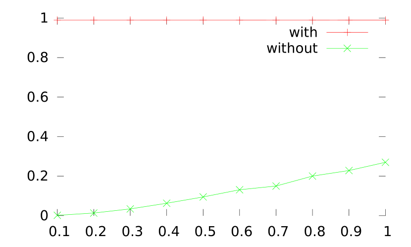
$\beta=1.1$		$\beta=2.6$
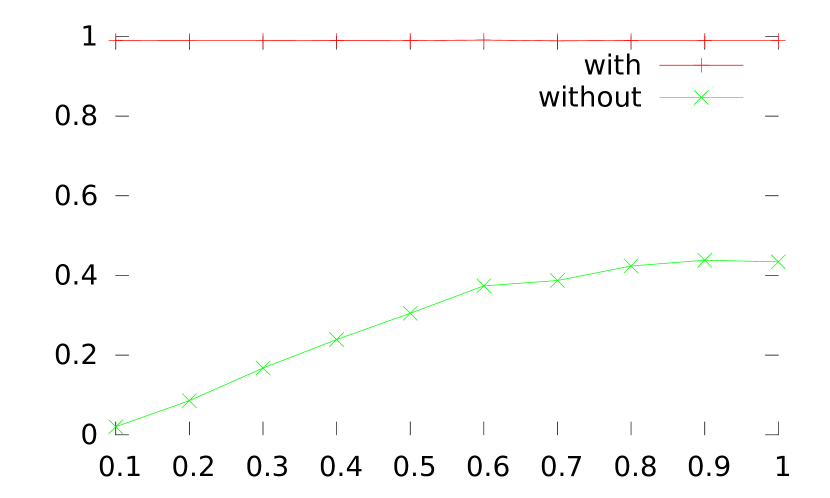
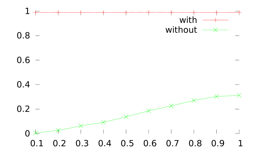
$\beta=1.4$		$\beta=2.9$
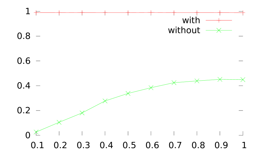
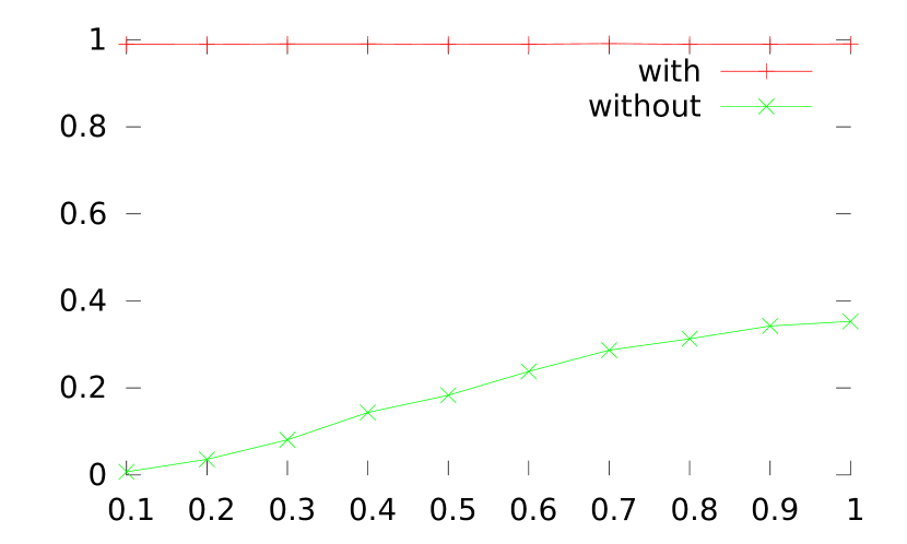
$\beta=1.7$		$\beta=3.2$

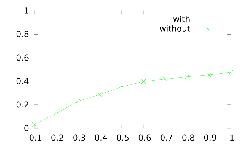
Figure 5: Proportion of job pairs (vertical axis) that satisfy a global precedence relation as function of the parameter $\sigma$ (horizontal axis). For every $(\beta,\sigma)$ pair, 25 instances, each contains 60 jobs, have been tested (Sections 8.1 and 8.2).

As a measure of the hardness of instances, we consider the portion of job pairs $i,j$ which satisfy global precedence. By this we mean that we have either $i\prec_{g[0,t_{1}]}j$ or $j\prec_{g[0,t_{1}]}i$ for $t_{1}$ being the total processing time over all jobs excepting jobs $i,j$. Figure 5 shows this measure for various choices of $\beta$.

The results depicted in Figure 5 confirm the choice of the model of random instances. Indeed the hardness of the instances seems to depend only little on $\beta$, except for $\beta=2$ where particularly strong precedence rules have been established. In addition the impact of our new rules is significant, and further experiments show how this improvement influences the number of generated nodes, and therefore the running time. Moreover it is quite visible from the measures that the instances are more difficult to solve when they are generated with a small $\sigma$ value.

8.3 Comparison between forward and backward approaches

In this section, we consider a variant of the algorithm. The algorithm described so far is called the backward approach, and the variant is called the forward approach. Here a partial schedule describes a prefix of length $t$ of a complete schedule and is extended to its right along an edge of the search tree, and in this variant the basic lower bound is $h(S):=\sum_{i\in S}w_{i}(t+p_{i})^{\beta}$. However in the backward approach, a partial schedule $S$ describes a suffix of a complete schedule and is extended to its left. For this variant, we choose $h(S):=\sum_{i\in S}w_{i}p_{i}^{\beta}$. Kaindl et al (2001) give experimental evidence that the backward variant generates for some problems less nodes in the search tree, and this fact has also been observed by Höhn and Jacobs (2012a).

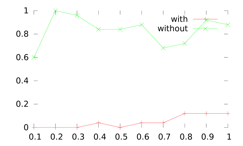
$\beta=0.5$		$\beta=2.0$
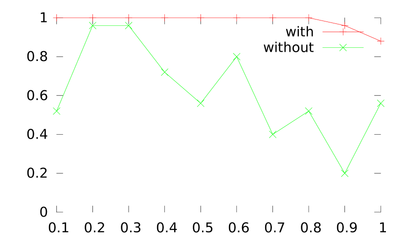
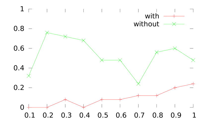
$\beta=0.8$		$\beta=2.3$
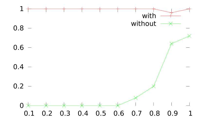
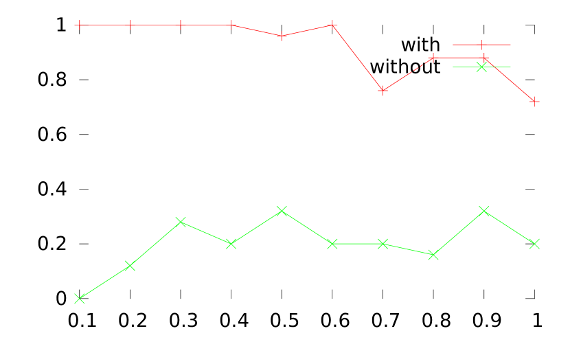
$\beta=1.1$		$\beta=2.6$
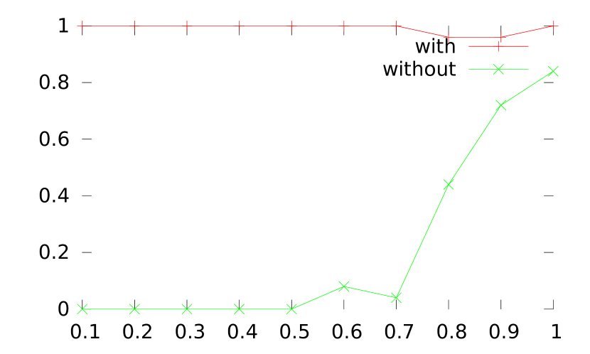
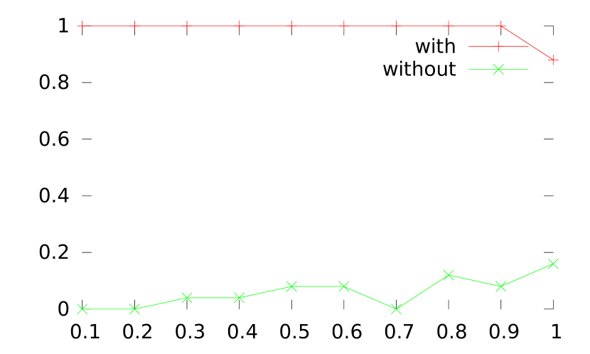
$\beta=1.4$		$\beta=2.9$
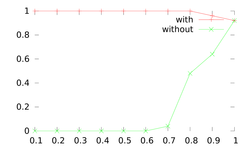
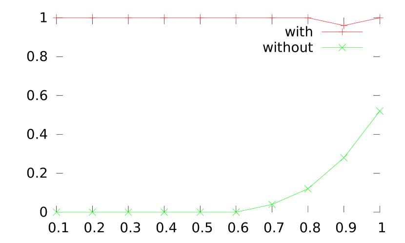
$\beta=1.7$		$\beta=3.2$

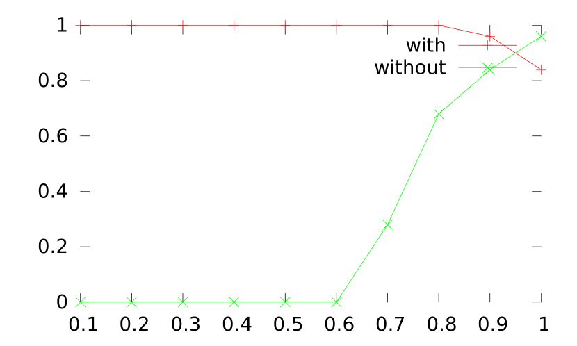
Figure 6: Proportion of instances (vertical axis) for which the forward variant generated less nodes than the backward variant. The values are plotted as function of $\sigma$ (horizontal axis) with and without our new rules (Section 8.3). For every $(\beta,\sigma)$ pair, 25 instances, each contains 20 jobs, have been tested.

We conducted an experimental study in order to find out which variant is most likely to be more efficient. The results are shown in Figure 6. The values are most significative for small $\sigma$ values, since for large values the instances are easy anyway and the choice of the variant is not very important. The results indicate that without our rules the forward variant should be used only when $\beta<1$ or $\beta=2$, while with our rules the forward variant should be used only when $\beta>1$.

Later on, when we measured the impact of our rules in the subsequent experiments, we compared the behavior of the algorithm using the most favorable variant dependent on the value of $\beta$ as described above.

8.4 Timeout

During the resolution a timeout was set, aborting executions that needed more than a million nodes. In Figure 4 we show the fraction of instances that could be solved within the limited number of nodes. From these experiments we measure the instance sizes that can be efficiently solved, and observe that this limit is of course smaller when $\sigma$ is small, as the instances become harder. But we also observe that with the usage of our rules much larger instances can be solved.

When $\beta$ is close to $1$, and instances consist of jobs of almost equal Smith-ratio, the different schedules diverge only slightly in cost, and intuitively one has to develop a schedule prefix close to the makespan, in order to find out that it cannot lead to the optimum. However for $\beta=2$, the Mondal-Sen-Höhn-Jacobs conditions make the instances easier to solve than for other values of $\beta$, even close to $2$. Note that we had to consider different instance sizes, in order to obtain comparable results, as with our rules all 20 job instances could be solved.

Figure 4: Proportion of instances which could be solved within the imposed time limit of a million nodes, with (below) and without (above) the new rules. For every $(\beta,\sigma)$, the evaluation is done on 25 instances each consists of 40 random jobs.

8.5 Improvement factor

In this section we measure the influence on the number of nodes generated during a resolution when our rules are used. For $\beta=2$ we compare our performance with the Mondal-Sen-Höhn-Jacobs conditions defined in (Mondal and Sen 2000) and proved in (Höhn and Jacobs 2012a), while for other values of $\beta$ we compare with the Sen-Dileepan-Ruparel condition defined in (Sen et al 1990). For fairness we excluded instances where the timeout was reached without the use of our rules. Figure 7 shows the ratio between the average number of generated nodes when the algorithm is run with our rules, and when it is run without our rules. Clearly this factor is smaller for $\beta=2$, since the Mondal-Sen-Höhn-Jacobs conditions apply here.

We observe that the improvement factor is more significant for hard instances, i.e.  when $\sigma$ is small. From the figures it seems that this behavior is not monotone, for $\beta=1.1$ the factor is less important with $\sigma=0.1$ than with $\sigma=0.3$. However this is an artifact of our pessimistic measurements, since we average only over instances which could be solved within the time limit, so in the statistics we filtered out the really hard instances.

9 Performance measurements for $\beta=2$

For $\beta=2$, Höhn and Jacobs (2012a) provide several test sets to measure the impact of their rules in different variants, see Höhn and Jacobs (2012b). For completeness we selected two data sets from their collection to compare our rules with theirs.

The first set called set-n contains for every number of jobs $n=1,2,\ldots,35$, 10 instances generated with parameter $\sigma=0.5$. This test set permits to measure the impact of our rules as a function of the instance size.

The second test set that we considered is called set-T and contains 3 instances of 25 jobs for every parameter

$$\sigma=0.100,0.101,0.102,\ldots,1.000.$$

Results are depicted in Figure 8, and show an improvement in the range of one order of magnitude.

10 Performance depending on input size

In addition we show the performance of the algorithm with our rules, in dependence on the number of jobs. Figure 9 shows for different number of jobs the number of generated nodes averaged over 100 instances generated with different $\sigma$ parameters, exposing an expected running time which strongly depends on the hardness of the instances.

11 Conclusion

We formulated the local global conjecture for the single machine scheduling problem of minimizing $w_{j}C_{j}^{\beta}$ for any positive constant $\beta$. We proved it for $\beta\geq 1$ substantially extending and improving over previous partial results. We also show some partial results for the remaining case $0<\beta<1$.

We conducted experiments and measured the impact of our conditions on the running time (number of generated nodes) by an A* based exact resolution. Improvements by a factor up to 1e4 have been observed.

Based on extensive experiments we believe that the conjecture should also hold in this case. However, it seems to be substantially more complicated and new analytical techniques seem to be necessary. We also describe a more general class of functions for which our results hold. Determining the class of objective functions for which the local global conjecture holds would also be a very interesting direction to explore.

Acknowledgements

We are grateful to the anonymous referees who spotted errors in previous versions of this paper. This paper was supported by the PHC Van Gogh grant 33669TC, the FONDECYT grant 11140566, the NWO grant 639.022.211 and the ERC consolidator grant 617951.

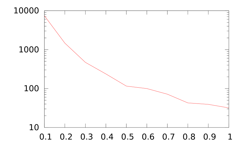
$\beta=0.5$		$\beta=2.0$
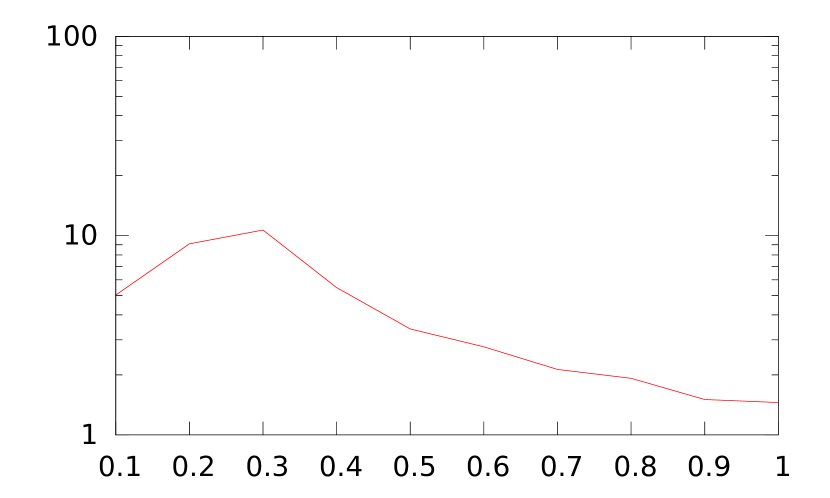
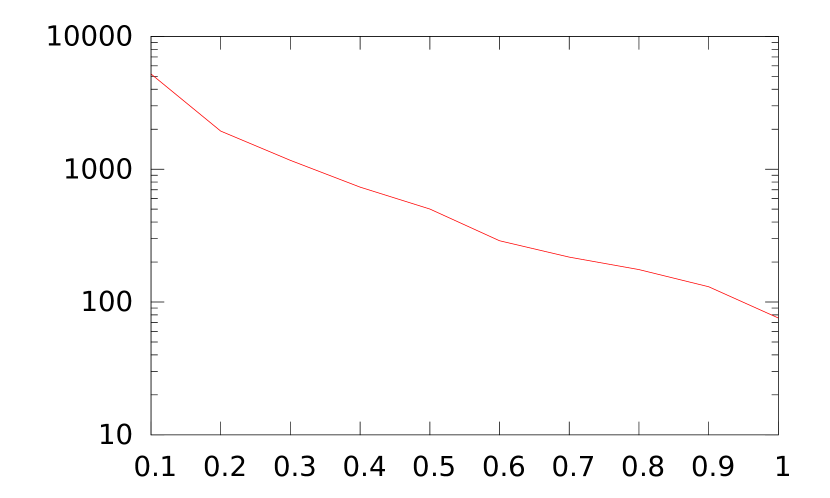
$\beta=0.8$		$\beta=2.3$
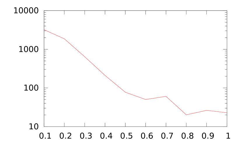
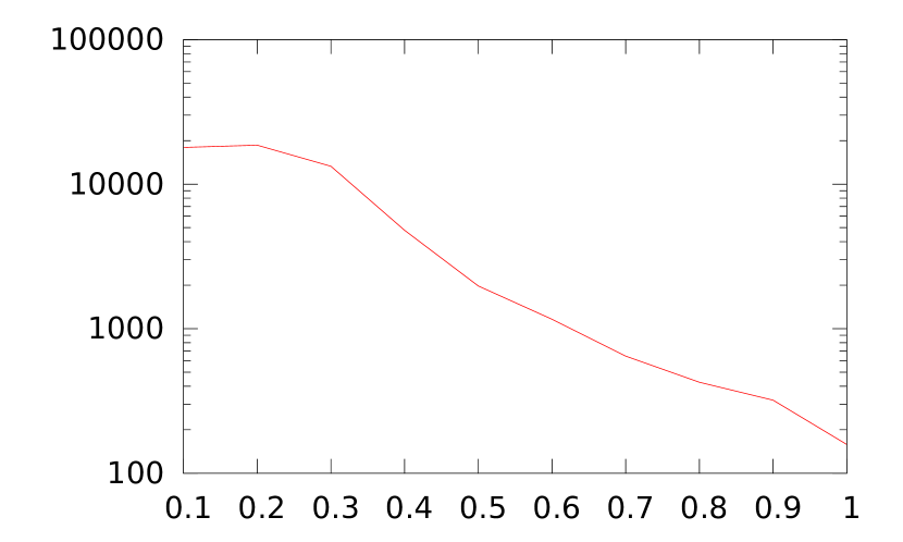
$\beta=1.1$		$\beta=2.6$
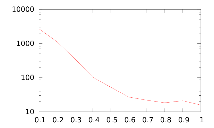
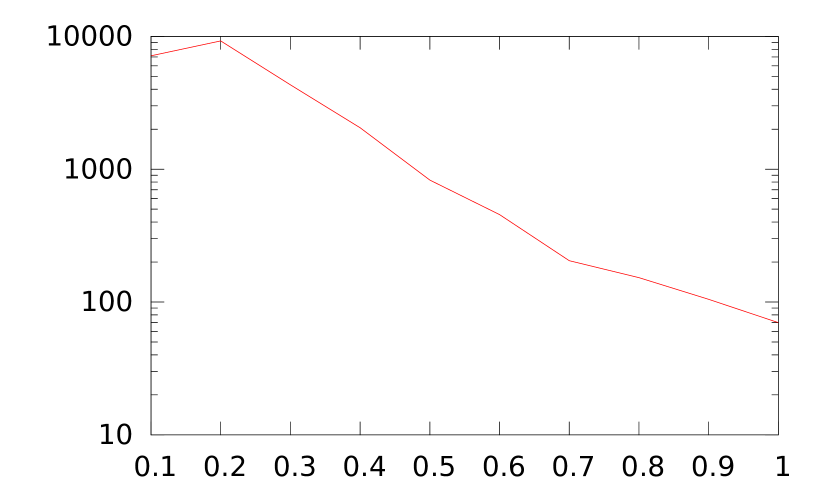
$\beta=1.4$		$\beta=2.9$
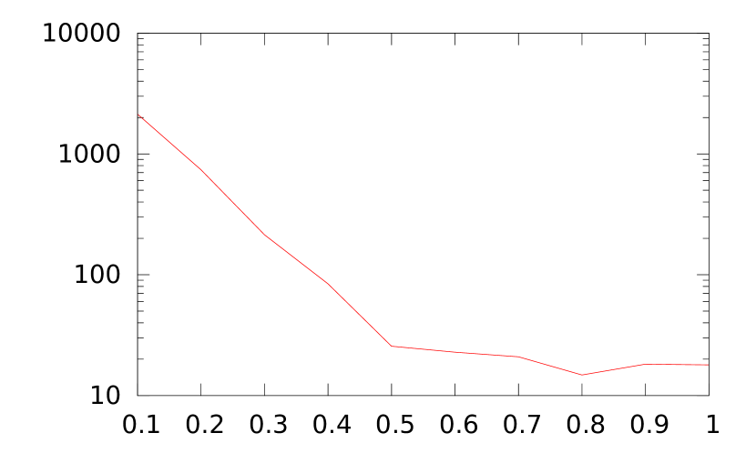
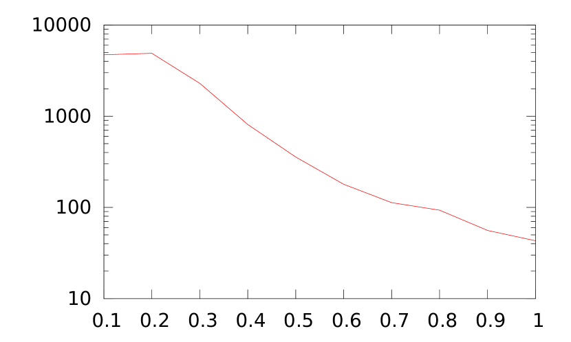
$\beta=1.7$		$\beta=3.2$

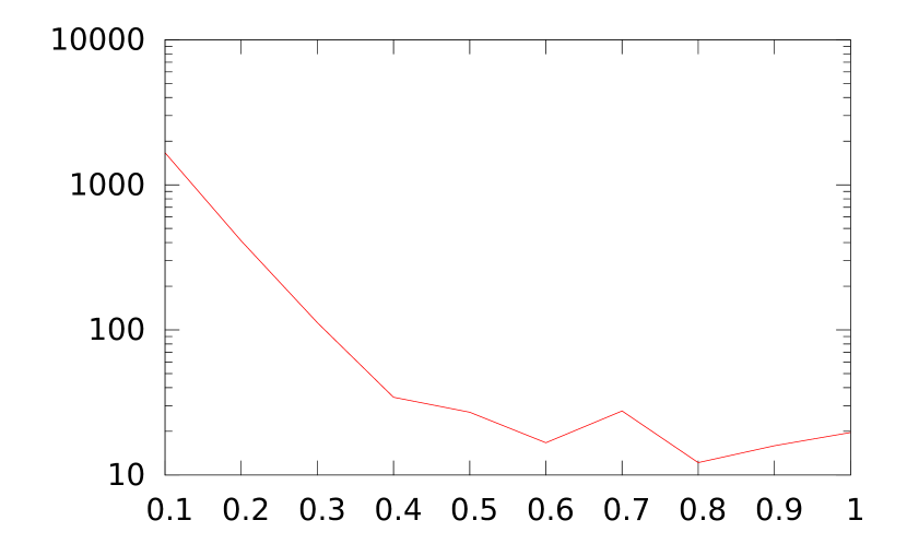
Figure 7: Average improvement factor (vertical axis) as function of $\beta$ and $\sigma$ (horizontal axis). For every $(\beta,\sigma)$ pair, 25 instances, each contains 20 jobs, have been tested (Section 8.5).

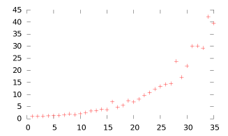
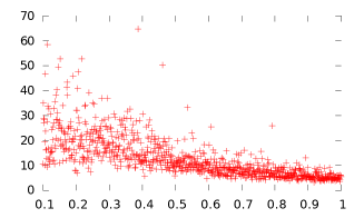
Figure 8: Improvement ratio for test sets set-n (left) and set-T (right) (Section 9).

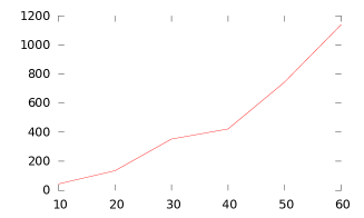
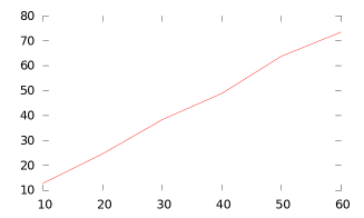
Figure 9: Average number of nodes (vertical axis) in dependance on the size (horizontal axis) of the instances, generated with $\beta=2$ and $\sigma=0.1$ on the left and $\sigma=0.5$ on the right (Section 10).

References

- Alidaee (1993) Alidaee B (1993) Numerical methods for single machine scheduling with non-linear cost functions to minimize total cost. Journal of the Operational Research Society 44(2):125–132
- Bagga and Karlra (1980) Bagga P, Karlra K (1980) A node elimination procedure for Townsend’s algorithm for solving the single machine quadratic penalty function scheduling problem. Management Science 26(6):633–636
- Bansal and Pruhs (2010) Bansal N, Pruhs K (2010) The geometry of scheduling. In: Proc. of the IEEE 51st Annual Symposium on Foundations of Computer Science (FOCS), pp 407–414
- Cheung and Shmoys (2011) Cheung M, Shmoys D (2011) A primal-dual approximation algorithm for min-sum single-machine scheduling problems. In: Proc. of the 14th International Workshop APPROX and 15th International Workshop RANDOM, pp 135–146
- Croce et al (1993) Croce F, Tadei R, Baracco P, Di Tullio R (1993) On minimizing the weighted sum of quadratic completion times on a single machine. In: Proc. of the IEEE International Conference on Robotics and Automation, pp 816–820
- Dürr et al (2014) Dürr C, Jeż Ł, Vásquez OC (2014) Scheduling under dynamic speed-scaling for minimizing weighted completion time and energy consumption. Discrete Applied Mathematics 0, DOI http://dx.doi.org/10.1016/j.dam.2014.08.001
- Epstein et al (2010) Epstein L, Levin A, Marchetti-Spaccamela A, Megow N, Mestre J, Skutella M, Stougie L (2010) Universal sequencing on a single machine. In Proc of the 14th International Conference of Integer Programming and Combinatorial Optimization (IPCO) pp 230–243
- Hart et al (1972) Hart PE, Nilsson NJ, Raphael B (1972) Correction to a formal basis for the heuristic determination of minimum cost paths. ACM SIGART Bulletin 37:28–29
- Höhn and Jacobs (2012a) Höhn W, Jacobs T (2012a) An experimental and analytical study of order constraints for single machine scheduling with quadratic cost. In: Proc. of the 14th Workshop on Algorithm Engineering and Experiments (ALENEX’12), pp 103–117
- Höhn and Jacobs (2012b) Höhn W, Jacobs T (2012b) Generalized min sum scheduling instance library. “http://www.coga.tu-berlin.de/v-menue/projekte/complex_scheduling/generalized_min-sum_scheduling_instance_library/”
- Höhn and Jacobs (2012c) Höhn W, Jacobs T (2012c) On the performance of Smith’s rule in single-machine scheduling with nonlinear cost. In: Proc. of the 10th Latin American Theoretical Informatics Symposium (LATIN), pp 482–493
- Kaindl et al (2001) Kaindl H, Kainz G, Radda K (2001) Asymmetry in search. IEEE Transactions on Systems, Man, and Cybernetics, Part B: Cybernetics 31(5):791–796
- Megow and Verschae (2013) Megow N, Verschae J (2013) Dual techniques for scheduling on a machine with varying speed. In: Proc. of the 40th International Colloquium on Automata, Languages and Programming (ICALP), pp 745–756
- Mondal and Sen (2000) Mondal S, Sen A (2000) An improved precedence rule for single machine sequencing problems with quadratic penalty. European Journal of Operational Research 125(2):425–428
- Sen et al (1990) Sen T, Dileepan P, Ruparel B (1990) Minimizing a generalized quadratic penalty function of job completion times: an improved branch-and-bound approach. Engineering Costs and Production Economics 18(3):197–202
- Smith (1956) Smith WE (1956) Various optimizers for single-stage production. Naval Research Logistics Quarterly 3(1-2):59–66
- Szwarc (1998) Szwarc W (1998) Decomposition in single-machine scheduling. Annals of Operations Research 83:271–287
- Townsend (1978) Townsend W (1978) The single machine problem with quadratic penalty function of completion times: a branch-and-bound solution. Management Science 24(5):530–534
- Vásquez (2014) Vásquez OC (2014) For the airplane refueling problem local precedence implies global precedence. Optimization Letters pp 1–13