Helicoidal minimal surfaces of prescribed genus, II

Abstract: In this paper we prove that for each positive integer $g$, there exists a complete minimal surface of genus $g$ that is properly embedded in three-dimensional euclidean space and that is asymptotic to the helicoid.

1. Introduction

In this paper we prove

Theorem 1.

For each positive integer $g$, there exists a complete minimal surface of genus $g$ that is properly embedded in ${\mathbb{R}}^{3}$ and asymptotic to the helicoid.

Let ${\mathbb{S}}^{2}(r)$ be the round sphere of radius $r$. Helicoidal minimal surfaces in ${\mathbb{S}}^{2}(r)\times{\mathbb{R}}$ of prescribed genus have been constructed by the authors in [4]. We obtain helicoidal minimal surfaces in ${\mathbb{R}}^{3}$ of prescribed genus by letting the radius $r$ go to infinity.

Our model for ${\mathbb{S}}^{2}(r)$ is ${\mathbb{C}\,}\cup\{\infty\}$ with the conformal metric obtained by stereographic projection:

(1) $$\lambda^{2}|dz|^{2}\quad\mbox{ with }\lambda=\frac{2r^{2}}{r^{2}+|z|^{2}},$$

In this model, the equator is the circle $|z|=r$. Our model for ${\mathbb{S}}^{2}(r)\times{\mathbb{R}}$ is $({\mathbb{C}\,}\cup\{\infty\})\times{\mathbb{R}}$ with the metric

(2) $$\lambda^{2}|dz|^{2}+dt^{2},\quad(z,t)\in({\mathbb{C}\,}\cup\{\infty\})\times{\mathbb{R}}.$$

When $r\to\infty$, this metric converges to the euclidean metric $4|dz|^{2}+dt^{2}$ on ${\mathbb{C}\,}\times{\mathbb{R}}={\mathbb{R}}^{3}$. (This metric is isometric to the standard euclidean metric by the map $(z,t)\mapsto(2z,t)$.)

Let $H$ be the standard helicoid in ${\mathbb{R}}^{3}$, defined by the equation

$$x_{2}\cos x_{3}=x_{1}\sin x_{3}.$$

It turns out that $H$ is minimal for the metric (2) for any value of $r$, although not complete anymore (see Section 2 in [4]). We complete it by adding the vertical line $\{\infty\}\times{\mathbb{R}}$, and still denote it $H$. This is a complete, genus zero, minimal surface in ${\mathbb{S}}^{2}\times{\mathbb{R}}$.

The helicoidal minimal surfaces in ${\mathbb{S}}^{2}\times{\mathbb{R}}$ constructed by the authors in [4] have any prescribed genus. In this paper we only consider those of even genus, which have one additional symmetry (denoted $\mu_{E}$ below). Fix some positive integer $g$. For any radius $r>0$, there exist, by Theorem 1 in [4], two distinct helicoidal minimal surfaces of even genus $2g$ in ${\mathbb{S}}^{2}(r)\times{\mathbb{R}}$, which we denote $M_{+}(r)$ and $M_{-}(r)$. Each one has two ends (corresponding to the two ends of ${\mathbb{S}}^{2}(r)\times{\mathbb{R}}$), each asymptotic to $H$ or to a vertical translate of $H$.

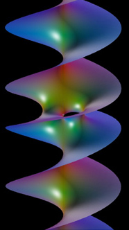
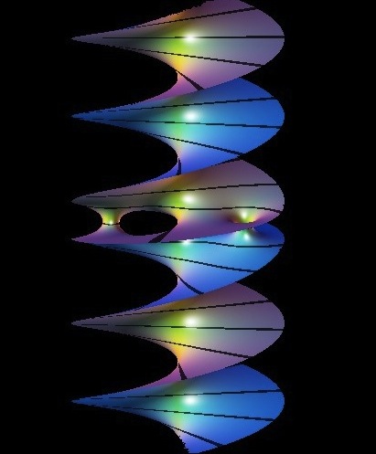
Figure 1. Left: A genus-one helicoid, computed by David Hoffman, Hermann Karcher and Fusheng Wei. Right: A genus-two helicoid, computed by Martin Traizet. Both surfaces were computed numerically using the Weierstrass representation and the images were made with Jim Hoffman using visualization software he helped to develop.

Regarding the limit as $r\to\infty$, the following result was already proved in [4], Theorem 2.

Theorem 2.

Let $s\in\{+,-\}$. Let $R_{n}$ be a sequence of radii diverging to infinity. A subsequence of the genus-$2g$ surfaces $M_{s}(R_{n})$ converges to a minimal surface $M_{s}$ in ${\mathbb{R}}^{3}$ asymptotic to the helicoid $H$. The convergence is smooth convergence on compact sets. Moreover,

• the genus of $M_{s}$ is at most $g$,

• the genus of $M_{+}$ is even,

• the genus of $M_{-}$ is odd,

• the number of points in $M_{s}\cap Y$ is $2\,\text{\rm genus}(M_{s})+1$.

The main result of this paper is the following theorem, from which Theorem 1 follows.

Theorem 3.

If $g$ is even, then $M_{+}$ has genus $g$. If $g$ is odd, then $M_{-}$ has genus $g$.

1.1. Pictures

A genus-2 helicoid was computed numerically by the second author in 1993 while he was a postdoc in Amherst (see Figure 1, right). Helicoids of genus up to six have been computed by Markus Schmies [6] using the theoretical techniques developed by Alexander Bobenko [2]. These surfaces were computed using the Weierstrass Representation and the Period Problem was solved numerically. There is of course no evidence that these numerically computed examples are the same as the ones obtained in Theorem 1, but they share the same symmetries. Pictures of these numerical examples suggest that an even genus helicoid looks like a helicoid with an even number of handles far from the axis, and an odd genus helicoid looks like a genus-one helicoid with an even number of handles far from the axis, the spacing between the handles getting larger and larger as the genus increases.

2. Preliminaries

2.1. Symmetries

Let us recall some notation from [4]. The real and imaginary axes in ${\mathbb{C}\,}$ are denoted $X$ and $Y$. The circle $|z|=r$ is denoted $E$ (the letter $E$ stands for “equator”). Note that $X$, $Y$ and $E$ are geodesics for the metric (1). We identify ${\mathbb{S}}^{2}$ with ${\mathbb{S}}^{2}\times\{0\}$, so $X$, $Y$ and $E$ are horizontal geodesics in ${\mathbb{S}}^{2}\times{\mathbb{R}}$. The antipodal points $(0,0)$ and $(\infty,0)$ are denoted $O$ and $O^{*}$ respectively. The vertical axes through $O$ and $O^{*}$ in ${\mathbb{S}}^{2}\times{\mathbb{R}}$ are denoted $Z$ and $Z^{*}$, respectively. If $\gamma$ is a horizontal or vertical geodesic in ${\mathbb{S}}^{2}\times{\mathbb{R}}$, the $180^{\circ}$ rotation around $\gamma$ is denoted $\rho_{\gamma}$. This is an isometry of ${\mathbb{S}}^{2}\times{\mathbb{R}}$. The reflection in the vertical cylinder $E\times{\mathbb{R}}$ is denoted $\mu_{E}$. This is an isometry of ${\mathbb{S}}^{2}\times{\mathbb{R}}$. In our model,

$$\mu_{E}(z,t)=\left(\frac{r^{2}}{\overline{z}},t\right).$$

The helicoid $H$ in ${\mathbb{S}}^{2}\times{\mathbb{R}}$ contains the geodesic $X$, the axes $Z$ and $Z^{*}$ and meets the geodesic $Y$ orthogonally at the points $O$ and $O^{*}$. It is invariant by $\rho_{X}$, $\rho_{Z}$, $\rho_{Z^{*}}$, $\mu_{E}$ (which reverse its orientation) and $\rho_{Y}$ (which preserves it).

The genus-$2g$ minimal surfaces $M_{+}(r)$ and $M_{-}(r)$ in ${\mathbb{S}}^{2}(r)\times{\mathbb{R}}$ have the following properties (see Theorem 1 of [4]):

Proposition 1.

Let $s\in\{+,-\}$. Then:

1. $M_{s}(r)$ is complete, properly embedded and has a top end and a bottom end, each asymptotic to $H$ or a vertical translate of $H$,

2. $M_{s}(r)\cap H=X\cup Z\cup Z^{*}$. In particular, $M_{s}(r)$ is invariant by $\rho_{X}$, $\rho_{Z}$ and $\rho_{Z^{*}}$, each of which reverses its orientation.

3. $M_{s}(r)$ is invariant by the reflection $\mu_{E}$, which reverses its orientation,

4. $M_{s}(r)$ meets the geodesic $Y$ orthogonally at $4g+2$ points and is invariant under $\rho_{Y}$, which preserves its orientation. Moreover, $(\rho_{Y})_{*}$ acts on $H_{1}(M_{s}(r),{\mathbb{Z}})$ by multiplication by $-1$.

2.2. Setup

Let $R_{n}$ be a diverging sequence of radii. By Theorem 2, a subsequence of $M_{s}(R_{n})$ (still denoted the same) converges to a helicoidal minimal surface $M_{s}$ that is helicoidal at infinity. Let $g^{\prime}$ be the genus of $M_{s}$. By the last point of Theorem 2, $M_{s}\cap Y$ has exactly $2g^{\prime}+1$ points. It follows that $2g^{\prime}+1$ points of $M_{s}(R_{n})\cap Y$ stay at bounded distance from the origin $O$. By $\mu_{E}$-symmetry, $2g^{\prime}+1$ points of $M_{s}(R_{n})\cap Y$ stay at bounded distance from the antipodal point $O^{*}$. There remains $4(g-g^{\prime})$ points in $M_{s}(R_{n})\cap Y$ whose distance to $O$ and $O^{*}$ is unbounded. Let

$$N=g-g^{\prime}.$$

We shall prove

Theorem 4.

In the above setup, $N\leq 1$.

Theorem 3 is a straightforward consequence of this theorem: Indeed if $g$ is even and $s=+$, we know by Theorem 2 that $g^{\prime}$ is even so $N=0$ and $g=g^{\prime}$. If $g$ is odd and $s=-$, then $g^{\prime}$ is odd so again $N=0$.

Remark 1.

If we let $M_{s}(r)\subset{\mathbb{S}}^{2}(r)\times{\mathbb{R}}$, $s\in\{+,-\}$ be the two helicoidal minimal surfaces of odd genus $2g+1$ constructed in [4] (instead of even genus), then $M_{+}(R_{n})$ will converge subsequentially to a minimal surface $M_{+}$ of even genus $g^{\prime}$ and $\mu_{E}(M_{+}(R_{n}))=M_{-}(R_{n})$ will converge subsequentially to a minimal surface $M_{-}$ of odd genus $g^{\prime\prime}$. Then there are $4g+2-2g^{\prime}-2g^{\prime\prime}=4N$ points on $M_{+}(R_{n})\cap Y$ whose distance to $O$ and $O^{*}$ is unbounded. Following our line of argument one should be able to prove that $N\leq 1$. This, however, does not determine $g^{\prime}$ nor $g^{\prime\prime}$, so is not enough to get the existence of helicoidal minimal surfaces in ${\mathbb{R}}^{3}$ of prescribed genus. This is the main reason why we only consider minimal surfaces of even genus in ${\mathbb{S}}^{2}\times{\mathbb{R}}$. The $\mu_{E}$ symmetry that these surfaces possess does make the proof somewhat simpler. The only point where we use it in a fundamental way is in the proof of Proposition 11 where we use Alexandrov reflection. Another argument would be required at this point in the odd-genus case.

To prove Theorem 4, assume that $N\geq 1$. We want to prove that $N=1$ by studying the $4N$ points whose distance to $O$ and $O^{*}$ is unbounded. To do this, it is necessary to work on a different scale. Let $R_{n}$ be a sequence of radii with $R_{n}\to\infty$. Define

$$M_{n}=\frac{1}{R_{n}}M_{s}(R_{n})\subset{\mathbb{S}}^{2}(1)\times{\mathbb{R}}.$$

This is a minimal surface in ${\mathbb{S}}^{2}(1)\times{\mathbb{R}}$. Each end of $M_{n}$ is asymptotic to a vertical translate of a helicoid of pitch

$$t_{n}=\frac{2\pi}{R_{n}}.$$

(The pitch of a helicoid with counterclockwise rotation is twice the distance between consecutive sheets. The standard helicoid has pitch $2\pi$.) Observe that $t_{n}\to 0$. By the definition of $N$, the intersection $M_{n}\cap Y$ has $4N$ points whose distance to $O$ and $O^{*}$ is $\gg t_{n}$. Because $M_{n}$ is symmetric with respect to $180^{\circ}$ rotation $\rho_{X}$ around $X$, there are $2N$ points on the positive $Y$-axis. We order these by increasing imaginary part:

$$p^{\prime}_{1,n},p^{\prime\prime}_{1,n},p^{\prime}_{2,n},p^{\prime\prime}_{2,n},\cdots,p^{\prime}_{N,n},p^{\prime\prime}_{N,n}.$$

Because of the $\rho_{X}$-symmetry, the $2N$ points on the negative $Y$-axis are the conjugates of these points. Define $p_{j,n}$ to be the midpoint of the interval $[p^{\prime}_{j,n},p^{\prime\prime}_{j,n}]$ and $r_{j,n}$ to be half the distance in the spherical metric from $p^{\prime}_{j,n}$ to $p^{\prime\prime}_{j,n}$. We have

$$0<\mbox{\rm\,Im\,}p_{1,n}<\mbox{\rm\,Im\,}p_{2,n}<\cdots<\mbox{\rm\,Im\,}p_{N,n}.$$

By $\mu_{E}$-symmetry, which corresponds to inversion in the unit circle,

(3) $$p_{N+1-i,n}=\frac{1}{\overline{p_{i,n}}}.$$

In particular, in case $N$ is odd, $p_{\frac{N+1}{2},n}=i$.

For $\lambda>1$ sufficiently large, let $\mathcal{Z}_{n}(\lambda)$ be the part of $M_{n}$ lying inside of the vertical cylinders of radius $\lambda t_{n}$ around $Z$ and $Z^{*}$:

(4) $$\mathcal{Z}_{n}(\lambda)=\{q=(z,t)\in M_{n}\,:\,d(Z\cup Z^{*},q)<\lambda t_{n}\}.$$

Also define $D_{j,n}(\lambda)=\{z\,:\,d(z,p_{j,n})<\lambda r_{j,n}\}$. Consider the intersection of $M_{n}$ with the vertical cylinder over $D_{j,n}(\lambda)$, and let $C_{j,n}(\lambda)$ denote the component of this intersection that contains the points $\{p^{\prime}_{j,n},p^{\prime\prime}_{j,n}\}$. Define

(5) $$\mathcal{C}_{n}(\lambda)=\bigcup_{j=1}^{N}C_{j,n}(\lambda)\cup\overline{C_{j,n}(\lambda)}.$$

The following proposition is key to setting up the analysis we will do in this paper to show that at most one handle is lost in taking the limit as $R_{n}\rightarrow\infty$. In broad terms, it says that near the points $p_{j,n}$, catenoidal necks are forming on a small scale, and after removing these necks and a neighborhood of the axes, what is left is a pair of symmetric surfaces which are vertical graphs over a half-helicoid.

Proposition 2.

Let $N=g-g^{\prime}$, $t_{n}$, and $M_{n}\subset{\mathbb{S}}^{2}(1)\times{\mathbb{R}}$, be as above. Then

1. For each $j$, $1\leq j\leq N$, the surface $\frac{1}{r_{j,n}}(M_{n}-p_{j,n})$ converges to the standard catenoid $\mathbf{C}$ with vertical axis and waist circle of radius $1$ in ${\mathbb{R}}^{3}$. In particular, the distance (in the spherical metric) $d(p_{j,n},p_{j+1,n})$ is $\gg r_{j,n}$. Moreover, $t_{n}\gg r_{j,n}$ and the $C_{j,n}(\lambda)$ are close to catenoidal necks with collapsing radii.

2. Given $\epsilon>0$, there exists a $\lambda>0$ such that

   $$M_{n}^{\prime}=M_{n}\setminus(\mathcal{Z}_{n}(\lambda)\cup\mathcal{C}_{n}(\lambda))$$

   has the following properties

   1. The slope of the tangent plane at any point of $M^{\prime}_{n}$ is less than $\epsilon$.

   2. $M^{\prime}_{n}$ consists of two components related by the symmetry $\rho_{Y}$, rotation by $180^{\circ}$ around $Y$.

   3. $M^{\prime}_{n}$ intersects $t_{n}H$ in a subset of the axis $X$ and nowhere else, with one of its components intersecting in a ray of the positive $X$-axis, the other in a ray of $X^{-}$. Each component is graphical over its projection onto the half-helicoid (a component of $t_{n}H\setminus(Z\cup Z^{*})$) that it intersects.

This proposition is proved in Theorem 16.9 and Corollary 16.13 of [4]. The notations in [4] are slightly different: See Remark 2 below.

Passing to a subsequence, $p_{j}=\lim p_{j,n}\in i{\mathbb{R}}^{+}\cup\{\infty\}$ exists for all $j\in[1,N]$. We have $p_{1}\in[0,i]$, and we will consider the following three cases:

(6) $$\begin{array}[]{ll}\bullet&\text{Case 1: }p_{1}\in(0,i),\\ \bullet&\text{Case 2: }p_{1}=0,\\ \bullet&\text{Case 3: }p_{1}=i.\end{array}$$

We will see that Case 1 and Case 2 are impossible, and that $N=1$ in Case 3.

2.3. The physics behind the proof of Theorem 4

Theorem 4 is proved by evaluating the surface tension in the $Y$-direction on each catenoidal neck. Mathematically speaking, this means the flux of the horizontal Killing field tangent to the $Y$-circle in ${\mathbb{S}}^{2}\times{\mathbb{R}}$. On one hand, this flux vanishes at each neck by $\rho_{Y}$-symmetry (see Lemma 1). On the other hand, we can compute the limit $F_{i}$ of the surface tension on the $i$-th catenoidal neck (corresponding to $p_{i}=\lim p_{i,n}$) as $n\to\infty$, after suitable scaling.

Assume for simplicity that the points $O$, $p_{1},\cdots,p_{N}$ and $O^{*}$ are distinct. Recall that the points $p_{1},\cdots p_{N}$ are on the positive imaginary $Y$-axis. For $1\leq j\leq N$, let $p_{j}=iy_{j}$, with $0<y_{j}<\infty$. Then we will compute that

$$F_{i}=c_{i}^{2}\frac{1-y_{i}^{2}}{1+y_{i}^{2}}+\sum_{j=1\atop j\neq i}^{N}c_{i}c_{j}f(y_{i},y_{j})$$

where the numbers $c_{i}$ are positive and proportional to the size of the catenoidal necks and

$$f(x,y)=\frac{-2\pi^{2}}{(\log x-\log y)|\log x-\log y+i\pi|^{2}}.$$

Observe that $f$ is antisymmetric and $f(x,y)>0$ when $0<x<y$. We can think of the point $p_{i}$ as a particle with mass $c_{i}$ and interpret $F_{i}$ as a force of gravitation type. The particles $p_{1},\cdots,p_{N}$ are attracted to each other and we can interpret the first term by saying that each particle $p_{i}$ is repelled from the fixed antipodal points $O$ and $O^{*}$. All forces $F_{i}$ must vanish. It is physically clear that no equilibrium is possible unless $N=1$ and $p_{1}=i$. Indeed in any other case, $F_{1}>0$.

This strategy is similar to the one followed in [7] and [8]. The main technical difficulty is that we cannot guarantee that the points $O$, $p_{1},\cdots,p_{N}$ and $O^{*}$ are distinct. The distinction between Cases 1, 2 and 3 in (6) stems from this problem.

2.4. The space $\widetilde{{\mathbb{C}\,}^{*}}$

To compute forces we need to express $M_{n}$ as a graph. For this, we need to express the helicoid itself as a graph, away from its axes $Z$ and $Z^{*}$. Let $\widetilde{{\mathbb{C}\,}^{*}}$ be the universal cover of ${\mathbb{C}\,}^{*}$. Of course, one can identify $\widetilde{{\mathbb{C}\,}^{*}}$ with ${\mathbb{C}\,}$ by mean of the exponential function. It will be more convenient to see $\widetilde{{\mathbb{C}\,}^{*}}$ as the covering space obtained by analytical continuation of $\log z$, so each point of $\widetilde{{\mathbb{C}\,}^{*}}$ is a point of ${\mathbb{C}\,}^{*}$ together with a determination of its argument : points are couples $(z,\arg(z))$, although in general we just write $z$. The following two involutions of $\widetilde{{\mathbb{C}\,}^{*}}$ will be of interest:

• $(z,\arg(z))\mapsto(\overline{z},-\arg(z))$, which we write simply as $z\mapsto\overline{z}$. The fixed points are $\arg z=0$.

• $(z,\arg(z))\mapsto(1/\overline{z},\arg(z))$, which we write simply as $z\mapsto 1/\overline{z}$. The fixed points are $|z|=1$.

The graph of the function $\frac{t}{2\pi}\arg z$ on $\widetilde{{\mathbb{C}\,}^{*}}$ is one half of a helicoid of pitch $t$.

2.5. The domain $\Omega_{n}$ and the functions $f_{n}$ and $u_{n}$

By Proposition 2, away from the axes $Z\cup Z^{*}$ and the points $p_{j,n}$, we may consider $M_{n}$ to be the union of two multigraphs. We wish to express this part of $M_{n}$ as a pair of graphs over a subdomain of $\widetilde{{\mathbb{C}\,}^{*}}$. We will allow ourselves the freedom to write $z$ for a point $(z,\arg z)\in\widetilde{{\mathbb{C}\,}^{*}}$ when its argument is clear from the context. Thus we will write $p_{j,n}$ for the point $(p_{j,n},\pi/2)$ in $\widetilde{{\mathbb{C}\,}^{*}}$ corresponding to the points on $M_{n}\cap Y$ in Proposition 2. Define

(7) $$D_{n}(\lambda)=\{\,(z,\arg z)\,:\,|z|<\lambda t_{n}\text{ or }|z|>\frac{1}{\lambda t_{n}}\},$$

(8) $$D_{j,n}(\lambda)=\{\,(z,\arg z)\,:\,d(p_{j,n},z)<\lambda r_{j,n}\text{ and }0<\arg z<\pi\}$$

and

(9) $$\Omega_{n}=\Omega_{n}(\lambda)=\widetilde{{\mathbb{C}\,}^{*}}\setminus\left(D_{n}(\lambda)\cup\bigcup_{j=1}^{N}D_{j,n}(\lambda)\cup\overline{D_{j,n}(\lambda)}\right).$$

According to Statement $ii.$ of Proposition 2, there exists a $\lambda>0$ such that for sufficiently large $n$,

$$M^{\prime}_{n}=M_{n}\cap(\Omega_{n}(\lambda)\times{\mathbb{R}})$$

is the union of two graphs related by $\rho_{Y}$-symmetry, and each graph intersects the helicoid of pitch $t_{n}$ in a subset of the $X$-axis. Only one of these graphs can contain points on the positive $X$-axis. We choose this component and write it as the graph of a function $f_{n}$ on the domain $\Omega_{n}$. We may write

(10) $$f_{n}(z)=\frac{t_{n}}{2\pi}\arg z-u_{n}(z).$$

The function $u_{n}$ has the following properties:

(11) $$\begin{array}[]{ll}\bullet&\text{ $u_{n}(\overline{z})=-u_{n}(z)$. In particular, $u_{n}=0$ on $\arg z=0$.}\\ \bullet&\text{$u_{n}(1/\overline{z})=u_{n}(z)$ In particular, $\partial u_{n}/\partial\nu=0$ on $|z|=1$.}\\ \bullet&\text{ $0<u_{n}<t_{n}/2$ when $\arg z>0$.}\end{array}$$

The first two assertions follow from the symmetries of $M_{n}$. See Proposition 1 (Statements 2 and 3), and the discussion preceding it. The third assertion follows Proposition 2, Statement  $ii.c$, which implies that

$$0<|u_{n}|<t_{n}/2$$

when $\arg z>0$, since the vertical distance between the sheets of $t_{n}H$ is equal to $t_{n}/2$. Now choose a point $z_{0}$ in the domain of $f_{n}$ that is near the a point $p_{j,n}$. Then $|f_{n}(z_{0})|$ is small, and $\arg z_{0}$ is near $\pi/2$. Hence $f_{n}(z_{0})\sim t_{n}/4-u_{n}(z_{0})$, which implies that $u_{n}(z_{0})>0$. We conclude that $0<u_{n}<t_{n}/2$ when $\arg z>0$, as claimed.

Figure 2. The domain $\Omega_{n}$ in polar coordinates, $z=re^{i\theta}$. The function $u_{n}$ is positive for $\theta>0$. The line $r=1$ corresponds to the unit circle $|z|=1$. The white strip on the left corresponds to the projection of the vertical cylinder of radius $\lambda t_{n}$ about the $Z$-axis, and the region to the right of the shaded domain is its image by the inversion through the unit circle. The small disks correspond to the vertical cylinders of radius $\lambda r_{j,n}$ (in the spherical metric).

Remark 2.

There are some notational differences between [4] and the present paper:

• In [4], $z$ denotes the third coordinate in ${\mathbb{R}}^{3}$. Here $z=x+iy$ is a complex variable.

• In [4], the pitch of a helicoid is denoted $2\eta$. Here it is denoted $t$.

• In Section 16 of [4], the angle $\theta$ is measured from the positive $Y$-axis, whereas here, it is measured from the positive $X$-axis.

• The conformal factor for the spherical metric in [4] is slightly different from (1). It is chosen there so that it converges to $1$ as $r\to\infty$.

• In paper [4], $M_{s}(r)$ has genus $g$, whereas here it has genus $2g$.

2.6. Organization of the paper

We deal with Cases 1, 2 and 3, as listed in (6), separately. In each case, we first state, without proof, a proposition which describes the asymptotic behavior of the function $u_{n}$ defined by (10) as $n\to\infty$. We use this result to compute forces and obtain the required result (namely, $N=1$ or a contradiction). Then, we prove the proposition. Finally, an Appendix contains analytic and geometric results relevant to minimal surfaces in ${\mathbb{S}}^{2}\times{\mathbb{R}}$, which are used in this paper.

3. Case 1: $p_{1}\in(0,i)$

For $p\in\widetilde{{\mathbb{C}\,}^{*}}$, let $h_{p}$ be the harmonic function defined on $\widetilde{{\mathbb{C}\,}^{*}}\setminus\{p,\overline{p}\}$ by

(12) $$h_{p}(z)=-\log\left|\frac{\log z-\log p}{\log z-\log\overline{p}}\right|.$$

Note that since $p$ and $z$ are in $\widetilde{{\mathbb{C}\,}^{*}}$, both come with a determination of their logarithm, so the function $h_{p}$ is well defined. This function has the same symmetries as $u_{n}$:

(13) $$\begin{array}[]{ll}\bullet&h_{p}(\overline{z})=-h_{p}(z),\\ \bullet&h_{p}(1/\overline{z})=h_{1/\overline{p}}(z).\\ \bullet&\text{ Moreover, if $\arg p$ and $\arg z$ are positive then $h_{p}(z)>0$.}\end{array}$$

Remark 3.

The function $(z,p)\mapsto-h_{p}(z)$ is the Green function of the domain $\arg z>0$ of $\widetilde{{\mathbb{C}\,}^{*}}$.

Recall that $p_{i}=\lim p_{i,n}$. It might happen that several points $p_{j}$ are equal to $p_{i}$. In this case, we say that we have a cluster at $p_{i}$. Let $m$ be the number of distinct points amongst $p_{1},\cdots,p_{N}$. Relabel the points so that $p_{1},\cdots,p_{m}$ are distinct and

$$\mbox{\rm\,Im\,}p_{1}<\mbox{\rm\,Im\,}p_{2}\cdots<\mbox{\rm\,Im\,}p_{m}.$$

(In other words, we have selected one point in each cluster.) Let us define

(14) $$\widetilde{u}_{n}=\frac{|\log t_{n}|}{t_{n}}u_{n}.$$

Proposition 3.

Assume that $p_{1}\neq 0$. Then there exists a subsequence and non-negative real numbers $c_{0},\cdots,c_{m}$ such that

(15) $$\widetilde{u}(z):=\lim\widetilde{u}_{n}(z)=c_{0}\arg z+\sum_{i=1}^{m}c_{i}h_{p_{i}}(z).$$

The convergence is the usual smooth uniform convergence on compact subsets of $\widetilde{{\mathbb{C}\,}^{*}}$ minus the points $p_{i}$, $-p_{i}$ for $1\leq i\leq m$. Moreover, for $1\leq i\leq m$,

(16) $$c_{i}=\lim\frac{|\log t_{n}|}{t_{n}}\frac{\phi_{i,n}}{2\pi}$$

where $\phi_{i,n}$ is the vertical flux of $M_{n}$ on the graph of $f_{n}$ restricted to the circle $C(p_{i},\varepsilon)$ for a fixed, small enough $\varepsilon$.

In other words, $\phi_{i,n}$ is the sum of the vertical fluxes on the catenoidal necks corresponding to the points $p_{j,n}$ such that $p_{j}=p_{i}$.

Remark 4.

We allow $p_{1}=i$ as this proposition will be used in Case 3, Section 5.

This proposition is proved in Section 3.2 by estimating the Laplacian of $u_{n}$ and constructing an explicit barrier, from which we deduce that a subsequence converges to a limit harmonic function on $\widetilde{{\mathbb{C}\,}^{*}}$ with logarithmic singularities at $\pm p_{1},\cdots,\pm p_{m}$.

Remark 5.

In Proposition 3, it is easy to show using Harnack’s inequality that we can choose numbers $\lambda_{n}>0$ so that $\lambda_{n}u_{n}$ converges subsequentially to a nonzero limit of the form (15). (One fixes a point $z_{0}$ and lets $\lambda_{n}=1/u_{n}(z_{0})$.) However, for us it is crucial that we can choose $\lambda_{n}$ to be $\frac{|\log t_{n}|}{t_{n}}$; it means that in later calculations, we will be able to ignore terms that are $o(\frac{|\log t_{n}|}{t_{n}})$.

For all we know at this point, the limit $\widetilde{u}$ might be zero. We will prove this is not the case:

Proposition 4.

For each $i\in[1,m]$, $c_{i}>0$.

This proposition is proved in Section 3.3 using a height estimate, Proposition 19, to estimate the vertical flux of the catenoidal necks.

From now on assume that $p_{1}\in(0,i)$. Fix some small number $\varepsilon$ and let $F_{n}$ be the flux of the Killing field $\chi_{Y}$ on the circle $C(p_{1},\varepsilon)$. The field $\chi_{Y}$ is the Killing field associated with rotations with respect to poles whose equator is the $Y$-circle (see Proposition 17 in Appendix A.3). On one hand, we have:

Lemma 1.

$F_{n}=0$.

Proof.

Let $C_{n}$ be the graph of $f_{n}$ restricted to the circle $C(p_{1},\varepsilon)$. By Proposition 1, statement (4), $C_{n}$ together with its image $\rho_{Y}(C_{n})$ bound a compact region in $M_{n}$. Thus the flux of the Killing field $\chi_{Y}$ on $C_{n}\cup\rho_{Y}(C_{n})$ is $0$. By $\rho_{Y}$-symmetry, this flux is twice the flux $F_{n}$ of $\chi_{Y}$ on $C_{n}$. Thus $F_{n}=0$. ∎

On the other hand, $F_{n}$ can be computed using Proposition 18 from Appendix A.3:

$$F_{n} =-\mbox{\rm\,Im\,}\int_{C(p_{1},\varepsilon)}2\left(\frac{\partial}{\partial z}\left(\frac{t_{n}}{2\pi}\arg z-u_{n}\right)\right)^{2}\frac{i}{2}(1-z^{2})dz+O(t_{n}^{4})$$

$$=-\mbox{\rm\,Re\,}\int_{C(p_{1},\varepsilon)}\left(\frac{t_{n}}{4\pi iz}-u_{n,z}\right)^{2}(1-z^{2})dz+O(t_{n}^{4})$$

$$=-\mbox{\rm\,Re\,}\int_{C(p_{1},\varepsilon)}\left(\frac{-t_{n}^{2}}{16\pi^{2}z^{2}}-\frac{2t_{n}}{4\pi iz}u_{n,z}+(u_{n,z})^{2}\right)(1-z^{2})dz+O(t_{n}^{4})$$

(17) $$=\mbox{\rm\,Re\,}\int_{C(p_{1},\varepsilon)}\left(\frac{2t_{n}}{4\pi iz}u_{n,z}-(u_{n,z})^{2}\right)(1-z^{2})dz+O(t_{n}^{4})$$

The second equation comes from $\frac{\partial}{\partial z}\arg z=\frac{1}{2iz}$. The fourth equation is a consequence of the fact that $\frac{1-z^{2}}{z^{2}}$ has no residue at $p_{1}\neq 0$. The first term in (17) (the cross-product) is a priori the leading term. However we can prove that this term can be neglected:

Proposition 5.

(18) $$\lim\left(\frac{\log t_{n}}{t_{n}}\right)^{2}F_{n}=-\mbox{\rm\,Re\,}\int_{C(p_{1},\varepsilon)}(\widetilde{u}_{z})^{2}(1-z^{2})dz$$

where $\widetilde{u}$ is defined in (15) as the limit of $\frac{|\log t_{n}|}{t_{n}}u_{n}$.

This proposition is proved in Section 3.4 using a Laurent series expansion to estimate the first term in (17).

Assuming these results, we now prove

Proposition 6.

Case 1 is impossible.

Proof: According to Lemma 1, the flux $F_{n}$ is zero. Hence the limit in (18) is zero. We compute that limit and show that it is nonzero.

Differentiating equation (15), we get

$$\widetilde{u}_{z}=\frac{c_{0}}{2iz}-\sum_{i=1}^{m}\frac{c_{i}}{2z}\left(\frac{1}{\log z-\log p_{i}}-\frac{1}{\log z-\log\overline{p_{i}}}\right).$$

Therefore,

$$\mbox{\rm\,Res\,}_{p_{1}}(\widetilde{u}_{z})^{2}(1-z^{2})$$

$$= \mbox{\rm\,Res\,}_{p_{1}}\frac{1-z^{2}}{4z^{2}}\left[\frac{c_{1}^{2}}{(\log z-\log p_{1})^{2}}+2\frac{c_{1}}{\log z-\log p_{1}}\right.$$

$$\left.\left(\frac{-c_{0}}{i}-\frac{c_{1}}{\log z-\log\overline{p_{1}}}+\sum_{i=2}^{m}\frac{c_{i}}{\log z-\log p_{i}}-\frac{c_{i}}{\log z-\log\overline{p_{i}}}\right)\right]$$

$$= -\frac{c_{1}^{2}(1+p_{1}^{2})}{4p_{1}}+\frac{c_{1}(1-p_{1}^{2})}{2p_{1}}\left(\frac{-c_{0}}{i}-\frac{c_{1}}{\log p_{1}-\log\overline{p_{1}}}\right.$$

$$\left.+\sum_{i=2}^{m}\frac{c_{i}}{\log p_{1}-\log p_{i}}-\frac{c_{i}}{\log p_{1}-\log\overline{p_{i}}}\right).$$

(See Proposition 23 in Appendix A.6 for the residue computations.) Write $p_{j}=iy_{j}$ for $1\leq j\leq m$ so all $y_{j}$ are positive numbers. By Lemma 1, equation (18) and the Residue Theorem,

(19) $$0 = -\mbox{\rm\,Re\,}\int_{C(p_{1},\varepsilon)}(\widetilde{u}_{z})^{2}(1-z^{2})dz$$

$$= -\mbox{\rm\,Re\,}\left[2\pi i\frac{y_{1}^{2}+1}{4iy_{1}}\left(c_{1}^{2}\frac{y_{1}^{2}-1}{y_{1}^{2}+1}+2c_{1}\left(-\frac{c_{0}}{i}-\frac{c_{1}}{i\pi}\right.\right.\right.$$

$$\left.\left.\left.+\sum_{i=2}^{m}\frac{c_{i}}{\log y_{1}-\log y_{i}}-\frac{c_{i}}{\log y_{1}-\log y_{i}+i\pi}\right)\right)\right]$$

$$= \frac{\pi(y_{1}^{2}+1)}{2y_{1}}\left[c_{1}^{2}\frac{1-y_{1}^{2}}{y_{1}^{2}+1}+\sum_{i=2}^{m}\frac{-2\pi^{2}\,c_{1}c_{i}}{(\log y_{1}-\log y_{i})|\log y_{1}-\log y_{i}+i\pi|^{2}}\right].$$

Now $y_{1}<1$ and $y_{1}<y_{i}$ for all $i\geq 2$, so all terms in (19) are positive. This contradiction proves Proposition 6. $\Box$

Remark 6.

The bracketed term in (19) is precisely the expression for the force $F_{1}$ in Section 2.3.

3.1. Barriers

In this section we introduce various barriers that will be used to prove Proposition 3. Fix some $\alpha\in(0,1)$.

Definition 1.

$A_{n}$ is the set of points $(z,\arg z)$ in $\widetilde{{\mathbb{C}\,}^{*}}$ which satisfy $t_{n}^{\alpha}<|z|<1$ and $\arg z>0$, minus the disks $D(p_{i,n},t_{n}^{\alpha})$ for $1\leq i\leq N$.

It is clear that $A_{n}\subset\Omega_{n}$ for large $n$, since $t_{n}^{\alpha}\gg t_{n}$. Moreover, if $z\in A_{n}$ then $d(z,\partial\Omega_{n})\geq t_{n}^{\alpha}/2$.

Remark 7.

We work in the hemisphere $|z|\leq 1$ where the conformal factor of the spherical metric in (1) satisfies $1\leq\lambda\leq 2$. Hence euclidean and spherical distances are comparable. We will use euclidean distance. Also the euclidean and spherical Laplacians are comparable. The symbol $\Delta$ will mean euclidean Laplacian.

By the disk $D(p,r)$ in $\widetilde{{\mathbb{C}\,}^{*}}$ (for small $r$) we mean the points $(z,\arg z)$ such that $|z-p|<r$ and $\arg z$ is close to $\arg p$.

Let $\delta$ be the function on $A_{n}$ defined by

$$\delta(z)=\left\{\begin{array}[]{ll}\min\{|z|,|z-p_{1,n}|,\cdots,|z-p_{N,n}|\}&\mbox{ if }0<\arg z<\pi\\ |z|&\mbox{ if }\arg(z)\geq\pi\end{array}\right.$$

Lemma 2.

There exists a constant $C_{1}$ such that in the domain $A_{n}$, the function $u_{n}$ satisfies

$$|\Delta u_{n}|\leq C_{1}\frac{t_{n}^{3}}{\delta^{4}}$$

.

Proof: the function $f_{n}(z)=\frac{t_{n}}{2\pi}\arg z-u_{n}(z)$ satisfies the minimal surface equation, and $|\Delta f_{n}|=|\Delta u_{n}|$. The proposition then follows from Proposition 15 in Appendix A.1 (a straightforward application of Schauder estimate). More precisely:

• if $0<\arg z<\pi$, we apply Proposition 15 on the domain

  $$A^{\prime}_{n}=\{w\in\Omega_{n}\,:\,-\pi/2<\arg w<3\pi/2,|w|<2\}.$$

  The distance $d(z,\partial A^{\prime}_{n})$ is comparable to $\delta(z)$. The function $f_{n}$ is bounded by $3t_{n}/4$.

• If $k\pi\leq\arg z<k\pi+\pi$ for some $k\geq 1$, we apply Proposition 15 to the function $f_{n}-\frac{k}{2}t_{n}$ and the domain

  $$A^{\prime}_{n}=\{w\in\Omega_{n}\,:\,k\pi-\pi/2<\arg w<k\pi+3\pi/2,|w|<2\}.$$

  The distance $d(z,\partial A^{\prime}_{n})$ is comparable to $|z|$. The function $f_{n}-\frac{k}{2}t_{n}$ is again bounded by $3t_{n}/4$.

$\Box$

Next, we need to construct a function whose Laplacian is greater than $1/\delta^{4}$, in order to compensate for the fact that $u_{n}$ is not quite harmonic. Let $\chi:{\mathbb{R}}^{+}\to[0,1]$ be a fixed, smooth function such that $\chi\equiv 1$ on $[0,\pi]$ and $\chi\equiv 0$ on $[2\pi,\infty)$.

Lemma 3.

There exists a constant $C_{2}\geq 1$ such that the function $g_{n}$ defined on $A_{n}$ by

$$g_{n}(z)=\frac{C_{2}}{|z|^{2}}+\chi(\arg z)\sum_{i=1}^{N}\frac{1}{|z-p_{i,n}|^{2}}$$

satisfies

(20) $$\Delta g_{n}\geq\frac{4}{\delta^{4}}.$$

Moreover $\partial g_{n}/\partial\nu\leq 0$ on $|z|=1$ and

(21) $$g_{n}\leq\frac{C_{2}+N}{t_{n}^{2\alpha}}\quad\mbox{ in }A_{n}.$$

Proof: The inequality (21) follows immediately from the definitions of $g_{n}$ and $A_{n}$. The function $f$ defined in polar coordinate by $f(r,\theta)=1/r^{2}$ satisfies

$$|\nabla f|=\frac{2}{r^{3}},\qquad\Delta f=\frac{4}{r^{4}}.$$

Hence for $\arg z\geq 2\pi$, (20) is satisfied for any $C_{2}\geq 1$. Suppose $0<\arg z<\pi$. Then

$$\Delta g_{n}=\frac{4C_{2}}{|z|^{4}}+\sum_{i=1}^{N}\frac{4}{|z-p_{i,n}|^{4}}\geq\frac{4}{\delta^{4}}$$

so again, (20) is satisfied for any $C_{2}\geq 1$. If $\theta=\arg z\in[\pi,2\pi]$, we have $|z-p_{i,n}|\geq|z|=r$ and

$$|\nabla\chi(\arg z)|\leq\frac{C}{r},\qquad|\Delta\chi(\arg z)|\leq\frac{C}{r^{2}}.$$

Hence

$$\left|\Delta\frac{\chi(\arg z)}{|z-p_{i,n}|^{2}}\right|\leq\frac{C}{r^{2}}\frac{1}{r^{2}}+2\frac{C}{r}\frac{2}{r^{3}}+\frac{4}{r^{4}}.$$

Therefore, $\Delta g_{n}\geq 4/r^{4}$ provided $C_{2}$ is large enough. (The constant $C_{2}$ only depends on $N$ and a bound on $\chi^{\prime}$ and $\chi^{\prime\prime}$.) This completes the proof of (20). $\Box$

We need a harmonic function on $\widetilde{{\mathbb{C}\,}^{*}}$ that is greater than $|\log t|$ on $|z|=t$. A good candidate would be $-\log|z|$. However this function has the wrong Neumann data on the unit circle. We propose the following:

Lemma 4.

For $0<t<1$, the harmonic function $H_{t}(z)$ defined for $z\in\widetilde{{\mathbb{C}\,}^{*}}$, $\arg z>0$ by

$$H_{t}(z)=\mbox{\rm\,Im\,}\left(\frac{\log t\log z}{\log t+i\log z}\right)$$

has the following properties :

1. $H_{t}(z)>0$ if $\arg z>0$,

2. $H_{t}(1/\overline{z})=H_{t}(z)$, hence $\partial H_{t}/\partial\nu=0$ on $|z|=1$,

3. $H_{t}(z)\geq|\log t|/2$ if $|z|=t$,

4. for fixed $t$, $H_{t}(z)\geq|\log t|/2$ when $\arg z\to\infty$, uniformly with respect to $|z|$ in $t\leq|z|\leq 1$,

5. for fixed $z$, $H_{t}(z)\to\arg z$ when $t\to 0$,

6. $H_{t}(z)\leq|\log z|$ if $\arg z>0$.

Proof : it suffices to compute $H_{t}(z)$ in polar coordinates $z=re^{i\theta}$ :

$$H_{t}(z)=\frac{(\log t)^{2}\theta+|\log t|((\log r)^{2}+\theta^{2})}{(\log t-\theta)^{2}+(\log r)^{2}}.$$

The first two points follow. If $r=t$ then

$$H_{t}(z)=\frac{|\log t|}{2}\left(1+\frac{\theta^{2}}{2(\log t)^{2}+2|\log t|\theta+\theta^{2}}\right)\geq\frac{|\log t|}{2}$$

which proves point 3. If $t\leq r\leq 1$ then

$$H_{t}(z)\geq\frac{(\log t)^{2}\theta+|\log t|\theta^{2}}{(\log t-\theta)^{2}+(\log t)^{2}}$$

which gives point 4. Point 5 is elementary. For the last point, write

$$\left|\frac{\log t\log z}{\log t+i\log z}\right|\leq\left|\frac{\log t\log z}{\log t}\right|=|\log z|.$$

$\Box$

3.2. Proof of Proposition 3

The function $\widetilde{u}_{n}$ defined in (14) has the following properties in $A_{n}$:

(22) $$\begin{array}[]{ll}\bullet&\displaystyle|\Delta\widetilde{u}_{n}|\leq C_{1}\frac{t_{n}^{2}|\log t_{n}|}{\delta^{4}}\text{ by Lemma \ref{lemma1}},\\ \bullet&\widetilde{u}_{n}\leq|\log t_{n}|/2,\\ \bullet&\widetilde{u}_{n}=0\text{ on $\arg z=0$,}\\ \bullet&\partial\widetilde{u}_{n}/\partial\nu=0\text{ on $|z|=1$.}\end{array}$$

The last three properties follow from (11) and the fact that $A_{n}\subset\Omega_{n}$. Consider the barrier $v_{n}=v_{1,n}+v_{2,n}+v_{3,n}$ where

$$v_{1,n}(z)=-C_{1}t_{n}^{2}|\log t_{n}|g_{n}(z)+C_{1}(C_{2}+N)t_{n}^{2-2\alpha}|\log t_{n}|,$$

$$v_{2,n}(z)=\frac{1}{\alpha}\sum_{i=1}^{N}h_{p_{i,n}}(z)=-\frac{1}{\alpha}\sum_{i=1}^{N}\log\left|\frac{\log z-\log p_{i,n}}{\log z-\log\overline{p_{i,n}}}\right|,$$

$$v_{3,n}(z)=\frac{1}{\alpha}H_{t_{n}^{\alpha}}(z).$$

The function $v_{1,n}$ is positive in $A_{n}$ by the estimate (21) of Lemma 3. Observe that the second term in the expression for $v_{1,n}$ tends to $0$ as $n\to\infty$ since $\alpha<1$. The functions $v_{2,n}$ and $v_{3,n}$ are harmonic and positive in $A_{n}$ (see point (1) of Lemma 4 for $v_{3,n}$).

By (13) and the symmetry of the set $\{p_{1,n},\cdots,p_{N,n}\}$ (see (3)), the function $v_{2,n}$ satisfies $v_{2,n}(1/\overline{z})=v_{2,n}(z)$. Hence $\partial v_{2,n}/\partial\nu=0$ on the unit circle. By point (2) of Lemma 4, $\partial v_{3,n}/\partial\nu=0$ on the unit circle. Therefore by Lemma 3,

$$\frac{\partial v_{n}}{\partial\nu}=\frac{\partial v_{1,n}}{\partial\nu}\geq 0\text{ on $|z|=1$.}$$

Because $p_{i,n}\to p_{i}\neq 0$, we have on the circle $C(p_{i,n},t_{n}^{\alpha})$

$$\log|\log z-\log p_{i,n}|\simeq\log|z-p_{i,n}|$$

Hence for large $n$ and for $1\leq i\leq N$

$$v_{2,n}\geq\frac{1}{2\alpha}|\log t_{n}^{\alpha}|\geq\widetilde{u}_{n}\quad\mbox{ on }C(p_{i,n},t_{n}^{\alpha}).$$

Using point (3) of Lemma 4 and the second statement of (22), we have $v_{3,n}\geq\widetilde{u}_{n}$ on the boundary component $|z|=t_{n}^{\alpha}$. So we have

(23) $$\begin{array}[]{ll}\bullet&\Delta\widetilde{u}_{n}\geq\Delta v_{n}\text{ in $A_{n}$},\\ \bullet&\widetilde{u}_{n}\leq v_{n}\text{ on the boundaries $\arg z=0$, $|z|=t_{n}^{\alpha}$ and $C(p_{i,n},t_{n}^{\alpha})$,}\\ \bullet&\partial\widetilde{u}_{n}/\partial\nu\leq\partial v_{n}/\partial\nu\text{ on the boundary $|z|=1$},\\ \bullet&\widetilde{u}_{n}\leq v_{n}\text{ when $\arg z\to\infty$.}\end{array}$$

(The first statement follows from (20) and the first statement of (22).)

By the maximum principle, we have $\widetilde{u}_{n}\leq v_{n}$ in $A_{n}$.

For any compact set $K$ of the set $\{z\in\widetilde{{\mathbb{C}\,}^{*}}\,:\,|z|\leq 1,\arg z\geq 0\}\setminus\{p_{1},\cdots,p_{m}\}$, the function $v_{n}$ is bounded by $C(K)$ on $K$. (For $v_{3,n}$, use the last point of Lemma 4.) Then by symmetry, $u_{n}$ is bounded by $C(K)$ on $K\cup\overline{K}\cup\sigma(K)\cup\sigma(\overline{K})$, where $\sigma$ denotes the inversion $z\mapsto\overline{z}$. Let

$$\Omega_{\infty}=\lim_{n\to\infty}\Omega_{n}=\widetilde{{\mathbb{C}\,}^{*}}\setminus\{\pm p_{1},\cdots,\pm p_{m}\}.$$

Then $\widetilde{u}_{n}$ is bounded on compact subsets of $\Omega_{\infty}$. By standard PDE theory, passing to a subsequence, $\widetilde{u}_{n}$ has a limit $\widetilde{u}$. The convergence is the uniform smooth convergence on compact subsets of $\Omega_{\infty}$. The limit has the following properties

• $\widetilde{u}$ is harmonic in $\Omega_{\infty}$. This follows from the first point of (22).

• $\widetilde{u}(\overline{z})=-\widetilde{u}(z)$ and $\widetilde{u}(1/\overline{z})=\widetilde{u}(z)$.

• $\widetilde{u}(z)\geq 0$ if $\arg z\geq 0$.

Note that either $\widetilde{u}\equiv 0$ or $\widetilde{u}$ is positive in $\arg z>0$. Using the fact that $\log:\widetilde{{\mathbb{C}\,}^{*}}\to{\mathbb{C}\,}$ is biholomorphic, the following lemma tells us that $\widetilde{u}$ has the form given by equation (15).

Lemma 5.

Let $H$ be the upper half plane $\mbox{\rm\,Im\,}z>0$ in ${\mathbb{C}\,}$. Let $u$ be a positive harmonic function in $H\setminus\{q_{1},\cdots,q_{m}\}$ with boundary value $u=0$ on ${\mathbb{R}}$. Then there exists non-negative constants $c_{0},\cdots,c_{m}$ such that

$$u(z)=c_{0}\mbox{\rm\,Im\,}z-\sum_{i=1}^{m}c_{i}\log\left|\frac{z-q_{i}}{z-\overline{q_{i}}}\right|.$$

This lemma easily follows from the following two facts and the maximum principle:

• If $u$ is a positive harmonic function in the punctured disk $D(p,\varepsilon)\setminus\{p\}$ then $u(z)=-c\log|z-p|+v(z)$ where $v$ is harmonic in the disk. (Bôcher Theorem, [1], Theorem 3.9)

• If $u$ is a positive harmonic function in $H$ with boundary value $0$ on ${\mathbb{R}}$ then $u=c\mbox{\rm\,Im\,}z$. ([1], Theorem 7.22).

To conclude the proof of Proposition 3, it remains to compute the numbers $c_{i}$ for $1\leq i\leq m$. Recall that $\phi_{i,n}$ is the vertical flux of $M_{n}$ on the graph of $f_{n}$ restricted to the circle $C(p_{i},\varepsilon)$. By Proposition 18,

$$\phi_{i,n}=\mbox{\rm\,Im\,}\int_{C(p_{i},\varepsilon)}(2f_{n,z}+O(t_{n}^{2}))dz=\mbox{\rm\,Im\,}\int_{C(p_{i},\varepsilon)}(-2u_{n,z}+O(t_{n}^{2}))dz.$$

Now

$$\lim\frac{|\log t_{n}|}{t_{n}}u_{n}=-c_{i}\log|z-p_{i}|+\text{harmonic}\quad\text{ near $p_{i}$}.$$

$$\lim\frac{|\log t_{n}|}{t_{n}}2u_{n,z}=-\frac{c_{i}}{z-p_{i}}+\text{holomorphic}\quad\text{ near $p_{i}$}.$$

Hence by the Residue Theorem,

$$\lim\frac{|\log t_{n}|}{t_{n}}\phi_{i,n}=2\pi c_{i}.$$

This finishes the proof of Proposition 3. $\Box$

As a corollary of the proof of Proposition 3, we have an estimate of $u_{n}$ that we will need in Section 5.5. For convenience, we state it here as a lemma.

Fix some $\beta\in(0,\alpha)$ and let $A^{\prime}_{n}\subset A_{n}$ be the domain defined as $A_{n}$ in Definition 1, replacing $\alpha$ by $\beta$, namely: $A^{\prime}_{n}$ is the set of points $(z,\arg z)$ in $\widetilde{{\mathbb{C}\,}^{*}}$ which satisfy $t_{n}^{\beta}<|z|<1$ and $\arg z>0$, minus the disks $D(p_{i,n},t_{n}^{\beta})$ for $1\leq i\leq N$.

Lemma 6.

Assume that $p_{1}\neq 0$. Then for $n$ large enough (depending only on $\beta$ and a lower bound on $|p_{1}|$), we have

$$u_{n}\leq(N+2)\frac{\beta}{\alpha}t_{n}\quad\mbox{ in }A^{\prime}_{n}.$$

Recalling that $u_{n}<t_{n}/2$, this lemma is usefull when $\beta$ is small. We will use it to get information about the level sets of $u_{n}$.

Proof: as we have seen in the Proof of Proposition 3, we have in $A_{n}$

(24) $$u_{n}\leq\frac{t_{n}}{|\log t_{n}|}v_{n}=\frac{t_{n}}{|\log t_{n}|}(v_{1,n}+v_{2,n}+v_{3,n}).$$

We need to estimate the functions $v_{1,n}$, $v_{2,n}$ and $v_{3,n}$ in $A^{\prime}_{n}$. We have in $A_{n}$

$$v_{1,n}\leq C_{1}(C_{2}+N)t_{n}^{2-2\alpha}|\log t_{n}|=o(|\log t_{n}|).$$

By point 6 of Lemma 4, we have in $A^{\prime}_{n}$

$$v_{3,n}\leq\frac{1}{\alpha}|\log z|\leq\frac{1}{\alpha}|\log t_{n}^{\beta}|=\frac{\beta}{\alpha}|\log t_{n}|.$$

Regarding the function $v_{2,n}$, we need to estimate each function $h_{p_{i,n}}$ in the domain $A^{\prime}_{n}$. The function $h_{p_{i,n}}$ is harmonic in the domain

$$\{z\in\widetilde{{\mathbb{C}\,}^{*}}\,:\,\arg z>0,\,t_{n}^{\beta}<|z|<1\}\setminus D(p_{i,n},t_{n}^{\beta})$$

and goes to $0$ as $\arg z\to\infty$, so its maximum is on the boundary. Since $h_{p_{i,n}}(1/\overline{z})=h_{p_{i,n}}(z)$, the maximum is not on the circle $|z|=1$ (because it would be an interior maximum of $h_{p_{i,n}}$). Also $h_{p_{i,n}}=0$ on $\arg z=0$. Therefore, the maximum is either on $|z|=t_{n}^{\beta}$ or on the circle $C(p_{i,n},t_{n}^{\beta})$. On $|z|=t_{n}^{\beta}$, we have $h_{p_{i,n}}\to 0$ because $p_{i,n}$ is bounded away from $0$. On the circle $C(p_{i,n},t_{n}^{\beta})$, we have for $n$ large

$$\log z-\log p_{i,n}\simeq\frac{1}{p_{i,n}}(z-p_{i,n})$$

$$|\log z-\log p_{i,n}|\geq\frac{t_{n}^{\beta}}{2|p_{i,n}|}.$$

Hence

$$-\log|\log z-\log p_{i,n}|\leq\log(2|p_{i,n}|)+\beta|\log t_{n}|.$$

Also,

$$\log|\log z-\log\overline{p_{i,n}}|\leq\log(|\log z|+|\log p_{i,n}|)\simeq\log(2|\log p_{i,n}|).$$

Since $|p_{i,n}|$ is bounded away from $0$, this gives for $n$ large enough

$$h_{p_{i,n}}\leq C+\beta|\log t_{n}|\quad\text{ in $A^{\prime}_{n}$.}$$

Hence

$$v_{2,n}\leq C+N\frac{\beta}{\alpha}|\log t_{n}|.$$

Collecting all terms, we get, for $n$ large enough:

$$v_{n}\leq C+(N+1)\frac{\beta}{\alpha}|\log t_{n}|\leq(N+2)\frac{\beta}{\alpha}|\log t_{n}|\quad\text{ in $A^{\prime}_{n}$}.$$

Using (24), the lemma follows. $\Box$

3.3. Proof of Proposition 4

We continue with the notation of the end of the previous section. Fix some index $i$ and let $J=\{j\in[1,N]\,:\,p_{j}=p_{i}\}$. Passing to a subsequence, we may assume that

$$r_{i,n}=\max\{r_{j,n}\,:\,j\in J\}.$$

(The numbers $r_{j,n}$ have been defined in Section 2.2.) Fix some positive $\varepsilon$ such that $|p_{j}-p_{i}|\geq 2\varepsilon$ for $j\notin J$.

From Statement $i.$ of Proposition 2, we know that near $p_{j,n}$ the surface $M_{n}$ is close to a vertical catenoid with waist circle of radius $r_{j,n}$. More precisely, $\frac{1}{r_{j,n}}(M_{n}-p_{i,n})$ converges to the standard catenoid

$$x_{3}=\cosh^{-1}\sqrt{x_{1}^{2}+x_{2}^{2}}.$$

Since the vertical flux of the standard catenoid is $2\pi$, we have

(25) $$\phi_{i,n}\simeq 2\pi\sum_{j\in J}r_{j,n}\leq 2\pi|J|r_{i,n}.$$

Let

$$h_{j,n}=r_{j,n}\cosh^{-1}(2\lambda).$$

Observe that $h_{j,n}\ll t_{n}$. Consider the intersection of $M_{n}$ with the plane at height $h_{j,n}$ and project it on the horizontal plane. There is one component which is close to the circle $C(p_{j,n},2\lambda r_{j,n})$. We call this component $\gamma_{j,n}$. Observe that $\gamma_{j,n}\subset\Omega_{n}$ and $f_{n}=h_{j,n}$ on $\gamma_{j,n}$. Let $D_{j,n}$ be the disk bounded by $\gamma_{j,n}$.

We now estimate $f_{n}$ on the circle $C(p_{i,n},\varepsilon)$. By Proposition 3, we know that $|u_{n}|=O(\frac{t_{n}}{|logt_{n}|})$. Hence $f_{n}=\frac{t_{n}}{2\pi}\arg z-u_{n}(z)\sim\frac{t_{n}}{2\pi}\arg z$ on $C(p_{i,n},\varepsilon)$. Since $p_{i,n}$ is on the positive imaginary axis, $\arg z=\pi/2+O(\varepsilon)$ on $C(p_{i,n},\varepsilon)$. Hence$f_{n}(z)\sim\frac{t_{n}}{4}$ on $C(p_{i,n},\varepsilon)$. Consequently, the level set $f_{n}=\frac{t_{n}}{8}$ inside $\Omega_{n}\cap D(p_{i,n},\varepsilon)$ is a closed curve, possibly with several components. We select the component which encloses the point $p_{i,n}$ and call it $\Gamma_{n}$. (Note that by choosing a very slightly different height, we may assume that $\Gamma_{n}$ is a regular curve). Let $D_{n}$ be the disk bounded by $\Gamma_{n}$. Let

$$\Omega^{\prime}_{n}=D_{n}\setminus\bigcup_{j\in J}D_{j,n}$$

Then $\Omega^{\prime}_{n}\subset\Omega_{n}$. We are now able to apply the height estimate of Appendix A.4. We apply Proposition 19 with $r_{1}=\lambda r_{i,n}$, $r_{2}=\varepsilon$, $h=t_{n}/8-h_{i,n}\simeq t_{n}/8$ and $f$ equal to the function $f_{n}(z-p_{i,n})-t_{n}/8$. (Observe that by Proposition 2, Statement ${ii.}$, we may assume that $|\nabla f_{n}|\leq 1$. Also the fact that $\partial f_{n}/\partial\nu<0$ on $\gamma_{j,n}$ follows from the convergence to a catenoid.) We obtain

$$\frac{t_{n}}{8}-h_{i,n}\leq\frac{\sqrt{2}}{\pi}\phi_{i,n}\log\frac{\varepsilon}{\lambda r_{i,n}}.$$

Using (25), this gives for $n$ large enough

(26) $$\frac{t_{n}}{9}\leq\frac{\sqrt{2}}{\pi}\phi_{i,n}\log\frac{2\pi|J|\varepsilon}{\lambda\phi_{i,n}}$$

This implies

(27) $$\phi_{i,n}\geq\frac{2\pi|J|\varepsilon}{\lambda}t_{n}^{2}$$

for $n$ large. To see this, suppose that $\phi_{i,n}<\frac{2\pi|J|\varepsilon}{\lambda}t_{n}^{2}$. Substituting in (26), we get

$$C_{1}t_{n}\leq t_{n}^{2}|\log t_{n}|$$

for some constant $C_{1}>0$. This is clearly a contradiction since $t_{n}|\log t_{n}|\rightarrow 0$. Substitution of (27) in (26) gives

$$\frac{t_{n}}{9}\leq\frac{2\sqrt{2}}{\pi}\phi_{i,n}|\log t_{n}|$$

which implies that $\frac{|\log t_{n}|}{t_{n}}\phi_{i,n}$ is bounded below by a positive constant independent of $n$. Therefore, the coefficient $c_{i}$ defined in (16) is positive, as desired. $\Box$

Remark 8.

Together with (25), this gives

(28) $$r_{i,n}\geq\frac{1}{36|J|\sqrt{2}}\frac{t_{n}}{|\log t_{n}|}$$

for large $n$. This is a lower bound on the size of the largest catenoidal neck in the cluster corresponding to $p_{i}$. We have no lower bound for $r_{j,n}$ if $j\in J$, $j\neq i$. Conceptually, we could have $r_{j,n}=o(\frac{t_{n}}{|\log t_{n}|})$, although this seems unlikely.

3.4. Proof of Proposition 5

Let $g_{n}=u_{n,z}.$ We have to prove

$$\lim\left(\frac{\log t_{n}}{t_{n}}\right)^{2}\operatorname{Re}\int_{C(p_{1},\epsilon)}\frac{2t_{n}}{4\pi iz}u_{n,z}(1-z)^{2}\,dz=0,$$

i.e., that

$$\mbox{\rm\,Re\,}\int_{C(p_{1},\varepsilon)}\frac{1}{2iz}g_{n}(z)(1-z^{2})dz=o\left(\frac{t_{n}}{(\log t_{n})^{2}}\right).$$

Fix some $\alpha$ such that $0<\alpha<\frac{1}{2}$ and some small $\varepsilon>0$. Let $J$ be the set of indices such that $p_{j}=p_{1}$. Consider the domain

$$A_{n}=D(p_{1},\varepsilon)-\bigcup_{j\in J}D(p_{j,n},t_{n}^{\alpha})\subset\Omega_{n}.$$

By Proposition 15 in Appendix A.1, we have in $A_{n}$

$$|g_{n,\overline{z}}|=\frac{1}{4}|\Delta u_{n}|=\frac{1}{4}|\Delta f_{n}|\leq Ct_{n}^{3-4\alpha}.$$

$$|\nabla f_{n}|\leq Ct_{n}^{1-\alpha}.$$

As the gradient of $t_{n}\arg z$ is $O(t_{n})$ in $A_{n}$, this gives

$$|\nabla u_{n}|\leq Ct_{n}^{1-\alpha}.$$

Hence

(29) $$|g_{n}|\leq Ct_{n}^{1-\alpha}.$$

Proposition 21 gives us the formula

$$g_{n}(z)=g^{+}(z)+\sum_{j\in J}g_{j}^{-}(z)+\frac{1}{2\pi i}\int_{A_{n}}\frac{g_{n,\overline{z}}(w)}{w-z}dw\wedge\overline{dw}$$

where of course the functions $g^{+}$ and $g_{j}^{-}$ depend on $n$.

• The function $g^{+}$ is holomorphic in $D(p_{1},\varepsilon)$ so does not contribute to the integral.

• The last term is bounded by $Ct_{n}^{3-4\alpha}$. (The integral of $dw\wedge\overline{dw}/(w-z)$ is uniformly convergent.) Therefore we need $3-4\alpha>1$, namely $\alpha<\frac{1}{2}$ so that the contribution of this term to the integral is $o(t_{n}/(\log t_{n})^{2})$.

  Remark 9.

  This is a crude estimate. The laplacian $\Delta u_{n}$ is bounded by $Ct_{n}^{3}/d^{4}$, where $d$ is distance to the boundary. Integrating this estimate one get that this term is less than $Ct_{n}^{3-2\alpha}$, which is better. But one still needs $\alpha<1$ to ensure that this term is $o(t_{n}/(\log t_{n})^{2})$.

• Each function $f_{j}^{-}$ is expanded in series as in Proposition 21. By Proposition 22 in Appendix A.5, each residue $a_{j,1}$ is real. Hence

  (30) $$\mbox{\rm\,Re\,}\int_{C(p_{1},\varepsilon)}\frac{1}{2iz}\frac{a_{j,1}}{z-p_{j,n}}(1-z^{2})dz=a_{j,1}\mbox{\rm\,Re\,}\left(\frac{2\pi i}{2ip_{j,n}}(1-p_{j,n}^{2})\right)=0$$

  because $p_{j,n}$ is imaginary, so $a_{j,1}$ does not contribute to the integral.

• It remains to estimate the coefficients $a_{j,k}$ for $k\geq 2$. Using (29),

  $$|a_{j,k}|=\left|\frac{1}{2\pi i}\int_{C(p_{j,n},t_{n}^{\alpha})}g_{n}(z)(z-p_{j,n})^{k-1}dz\right|\leq Ct_{n}^{1+(k-1)\alpha}$$

  If $z\in C(p_{1},\varepsilon)$, then $|z-p_{j,n}|\geq\varepsilon/2$, so

  $$\left|\sum_{k=2}^{\infty}a_{j,k}(z-p_{j,k})^{-k}\right|\leq C\sum_{k\geq 2}t_{n}^{1+(k-1)\alpha}\left(\frac{2}{\epsilon}\right)^{k}\leq\frac{4C}{\varepsilon^{2}}t_{n}^{1+\alpha}\sum_{k=2}^{\infty}\left(\frac{2t_{n}^{\alpha}}{\varepsilon}\right)^{k-2}.$$

  The last sum converges because $\alpha>0$. Hence the contribution of this term to the integral is $o(t_{n}/(\log t_{n})^{2})$ as desired.

$\Box$

4. Case 2: $p_{1}=0$

In this case we make a blow up at the origin. Let

$$R_{n}=\frac{1}{|p_{1,n}|}$$

(Here we assume again that the points $p_{i,n}$ are ordered by increasing imaginary part as in Section 2.2.) Let $\widehat{M}_{n}=R_{n}M_{n}$. This is a helicoidal minimal surface in ${\mathbb{S}}^{2}(R_{n})\times{\mathbb{R}}$ with pitch

$$\widehat{t}_{n}=R_{n}t_{n}.$$

By choice of $p_{1,n}$, we have $|p_{1,n}|>>t_{n}$, so $\lim\widehat{t}_{n}=0$. Let $\widehat{\Omega}_{n}=R_{n}\Omega_{n}$. $\widehat{M}_{n}$ is the graph on $\widehat{\Omega}_{n}$ of the function

$$\widehat{f}_{n}(z)=\frac{\widehat{t}_{n}}{2\pi}\arg z-\widehat{u}_{n}(z)$$

where

$$\widehat{u}_{n}(z)=R_{n}u_{n}(\frac{z}{R_{n}}).$$

Let $\widehat{p}_{i,n}=R_{n}p_{i,n}$. Passing to a subsequence

$$\widehat{p}_{j}=\lim\widehat{p}_{j,n}\in[i,\infty]$$

exists for $j\in[1,N]$ and we have $\widehat{p}_{1}=i$. Let $m$ be the number of distinct, finite points amongst $\widehat{p}_{1},\cdots,\widehat{p}_{N}$. Relabel the points so that $\widehat{p}_{1},\cdots,\widehat{p}_{m}$ are distinct and

$$1=\mbox{\rm\,Im\,}\widehat{p}_{1}<\mbox{\rm\,Im\,}\widehat{p}_{2}<\cdots<\mbox{\rm\,Im\,}\widehat{p}_{m}.$$

Proposition 7.

Passing to a subsequence,

$$\lim\frac{|\log\widehat{t}_{n}|}{\widehat{t}_{n}}\widehat{u}_{n}(z)=\widehat{c}_{0}\arg z+\sum_{i=1}^{m}\widehat{c}_{i}h_{\widehat{p}_{i}}(z).$$

The convergence is the smooth uniform convergence on compact subsets of $\widetilde{{\mathbb{C}\,}^{*}}$ minus the points $\pm\widehat{p}_{i}$, for $1\leq i\leq m$. The numbers $\widehat{c}_{i}$ for $1\leq i\leq m$ are given by

$$\widehat{c}_{i}=\lim\frac{|\log\widehat{t}_{n}|}{\widehat{t}_{n}}\frac{\widehat{\phi}_{i,n}}{2\pi}$$

where $\widehat{\phi}_{i,n}$ is the vertical flux of $\widehat{M}_{n}$ on the graph of $\widehat{f}_{n}$ restricted to the circle $C(\widehat{p}_{i},\varepsilon)$, for some fixed small enough $\varepsilon$. Moreover, $\widehat{c}_{i}>0$ for $1\leq i\leq m$.

This proposition is proved in Section 4.1. The proof is very similar to the proof of Proposition 3, and Proposition 4 for the last statement.

Fix some small $\varepsilon>0$. Let $F_{n}$ be the flux of the Killing fields $\chi_{Y}$ on the circle $C(\widehat{p}_{1},\varepsilon)$ on $\widehat{M}_{n}$. Since we are in ${\mathbb{S}}^{2}(R_{n})\times{\mathbb{R}}$,

$$\chi_{Y}=\frac{i}{2}(1-\frac{z^{2}}{R_{n}^{2}}).$$

$$F_{n}=-\mbox{\rm\,Im\,}\int_{C(\widehat{p}_{1},\varepsilon)}2\left(\frac{\partial}{\partial z}\left(\frac{\widehat{t}_{n}}{2\pi}\arg z-\widehat{u}_{n}\right)\right)^{2}\frac{i}{2}\left(1-\frac{z^{2}}{R_{n}^{2}}\right)dz+O((\widehat{t}_{n})^{4}).$$

Expand the square. As in Case 1, the cross product term can be neglected and since $R_{n}\to\infty$:

Proposition 8.

$$\lim\left(\frac{\log\widehat{t}_{n}}{\widehat{t}_{n}}\right)^{2}F_{n}=-\lim\left(\frac{\log\widehat{t}_{n}}{\widehat{t}_{n}}\right)^{2}\mbox{\rm\,Re\,}\int_{C(\widehat{p}_{1},\varepsilon)}(\widehat{u}_{n,z})^{2}dz$$

(Same proof as Proposition 5).

Assuming these results, we now prove

Proposition 9.

Case 2 is impossible.

Proof: Write $\widehat{p}_{j}=iy_{j}$. By the same computation as in Section 3, we get (the only difference is that there is no $(1-z^{2})$ factor)

$$-\mbox{\rm\,Re\,}\int_{C(\widehat{p}_{1},\varepsilon)}(\widetilde{u}_{z})^{2}dz=\frac{\pi}{2y_{1}}\left(\widehat{c}_{1}^{2}+\sum_{i=2}^{m}\frac{-2\pi^{2}\,\widehat{c}_{1}\widehat{c}_{i}}{(\log y_{1}-\log y_{i})|\log y_{1}-\log y_{i}+i\pi|^{2}}\right).$$

Again, since $y_{i}>y_{1}$ for $i\geq 2$, all terms are positive, contradiction. $\Box$

4.1. Proof of Proposition 7

The setup of Proposition 7 is the same as Proposition 3 except that we are in ${\mathbb{S}}^{2}(R_{n})\times{\mathbb{R}}$ with $R_{n}\to\infty$ instead of ${\mathbb{S}}^{2}(1)\times{\mathbb{R}}$, and the pitch is $\widehat{t}_{n}$. Remember that $\lim\widehat{t}_{n}=0$.

From now on forget all hats: write $t_{n}$ instead of $\widehat{t}_{n}$, $u_{n}$ instead of $\widehat{u}_{n}$, $p_{i,n}$ instead of $\widehat{p}_{i,n}$, etc…

The proof of Proposition 7 is substantially the same as the proofs of Propositions 3 and 4. The main difference is that the equatorial circle $|z|=1$ becomes $|z|=R_{n}$.

• The definition of the domain $A_{n}$ is the same with $|z|<1$ replaced by $|z|<R_{n}$.

• Lemma 2 is the same (recall that now $p_{i,n}$ means $\widehat{p}_{i,n}$).

• Lemma 3 is the same. The last statement must be replaced by $\partial g_{n}/\partial\nu\leq 0$ on $|z|=R$ for $R\geq 1$.

• Lemma 4 is the same, we do not change the definition of the function $H_{t}$. Instead of point 3, we need $\partial H_{t}/\partial\nu\geq 0$ on $|z|=R$ for $R\geq 1$. This is true by the following computation:

  $$\frac{\partial H_{t}}{\partial r}=\frac{2\log r(\log t)^{2}(|\log t|+\theta)}{((\log t-\theta)^{2}+(\log r)^{2})^{2}}.$$

• The definition of the function $\widetilde{u}_{n}$ is the same, and it has the same properties, except that the last point must be replaced by $\partial\widetilde{u}_{n}/\partial\nu=0$ on $|z|=R_{n}$.

• The definition of the function $v_{2,n}$ is the same (with $\widehat{p}_{i,n}$ in place of $p_{i,n}$), now it is symmetric with respect to the circle $|z|=R_{n}$.

• At the end, $K$ is a compact of the set $\{z\in\widetilde{{\mathbb{C}\,}^{*}},\arg z\geq 0\}\setminus\{\widehat{p}_{1},\cdots,\widehat{p}_{m}\}.$ The fact that $v_{2,n}$ is uniformly bounded on $K$ requires some care, maybe, because some points $\widehat{p}_{i,n}$ are not bounded: it is true by the fact that if $\arg z$ and $\arg p$ are positive, then

  $$|\log z-\log p|\leq|\log z-\log\overline{p}|.$$

• The proof of the last point is exactly the proof of Proposition 4, working in ${\mathbb{S}}^{2}(R_{n})\times{\mathbb{R}}$ instead of ${\mathbb{S}}^{2}(1)\times{\mathbb{R}}$.

$\Box$

5. Case 3: $p_{1}=i$

Note that in this case, all points $p_{j,n}$ converge to $i$, for $j\in[1,N]$. We distinguish two sub-cases:

• Case 3a: there exists $\beta>0$ such that $|p_{1,n}-i|\leq t_{n}^{\beta}$ for $n$ large enough,

• Case 3b: for all $\beta>0$, $|p_{1,n}-i|\geq t_{n}^{\beta}$ for $n$ large enough.

(Here we assume again that the points $p_{i,n}$ are ordered by increasing imaginary part as in Section 2.2.) Roughly speaking, in Case 3a, all points $p_{j,n}$ converge to $i$ quickly, whereas in Case 3b, at least two ($p_{1,n}$ and $p_{N,n}$ by symmetry) converge to $i$ very slowly. We will see in Proposition 11 that $N=1$ and $p_{1,n}=i$ in Case 3a, and in Proposition 14 that Case 3b is impossible.

In both cases, we make a blowup at $i$ as follows : Let $\varphi:{\mathbb{S}}^{2}\to{\mathbb{S}}^{2}$ be the rotation of angle $\pi/2$ which fixes the $Y$ circle and maps $i$ to $0$. Explicitly, in our model of ${\mathbb{S}}^{2}(1)$

$$\varphi(z)=\frac{z-i}{1-iz},\qquad\varphi^{-1}(z)=\frac{z+i}{1+iz}.$$

It exchanges the equator $E$ and the great circle $X$. $\varphi$ lifts in a natural way to an isometry $\widehat{\varphi}$ of ${\mathbb{S}}^{2}\times{\mathbb{R}}$. We first apply the isometry $\widehat{\varphi}$ and then we scale by $1/\mu_{n}$ where the ratio $\mu_{n}$ goes to zero and will be chosen later, depending on the case. Let

$$\widehat{M}_{n}=\frac{1}{\mu_{n}}\widehat{\varphi}(M_{n})\subset{\mathbb{S}}^{2}(1/\mu_{n})\times{\mathbb{R}},$$

$$\widehat{\Omega}_{n}=\frac{1}{\mu_{n}}\varphi(\Omega),\qquad\widehat{p}_{i,n}=\frac{1}{\mu_{n}}\varphi(p_{i,n}),\qquad\widehat{t}_{n}=\frac{t_{n}}{\mu_{n}}.$$

The minimal surface $\widehat{M}_{n}$ is the graph over $\widehat{\Omega}_{n}$ of the function

$$\widehat{f}_{n}(z)=\frac{1}{\mu_{n}}f_{n}(\varphi^{-1}(\mu_{n}z))=\widehat{t}_{n}w_{n}(z)-\widehat{u}_{n}(z)$$

where

(31) $$w_{n}(z)=\frac{1}{2\pi}\arg\left(\frac{\mu_{n}z+i}{1+i\mu_{n}z}\right)$$

$$\widehat{u}_{n}(z)=\frac{1}{\mu_{n}}u_{n}(\varphi^{-1}(\mu_{n}z)).$$

5.1. Case 3a

In this case, fix some positive number $\alpha$ such that $\alpha<\min\{\beta,\frac{1}{8}\}$, and take $\mu_{n}=t_{n}^{\alpha}$. Then for all $j\in[1,N]$, $|p_{j,n}-i|=o(\mu_{n})$, so $\lim\widehat{p}_{j,n}=0$.

Proposition 10.

In Case 3a, passing to a subsequence,

(32) $$\lim\frac{|\log t_{n}|}{\widehat{t}_{n}}\left(\widehat{u}_{n}(z)-\widehat{u}_{n}(z_{0})\right)=-c(\log|z|-\log|z_{0}|).$$

The convergence is the uniform smooth convergence on compact subsets of ${\mathbb{C}\,}\setminus\{0\}$. (Here $z_{0}$ is an arbitrary fixed nonzero complex number.) The constant $c$ is positive.

The Proof is in Section 5.4.

Remark 10.

In fact

$$\lim\frac{|\log t_{n}|}{\widehat{t}_{n}}\widehat{u}_{n}(z)=\infty$$

for all $z$, so it is necessary to substract something to get a finite limit. Because of this, we believe it is not possible to prove this proposition by a barrier argument as in the proof of Proposition 3. Instead, we will prove the convergence of the derivative $\widehat{u}_{n,z}$ using the Cauchy Pompeieu integral formula for $C^{1}$ functions.

We now prove

Proposition 11.

In Case 3a, $N=1$.

Proof: From (31),

$$w_{n}(z)=\frac{1}{2\pi}\left(\frac{\pi}{2}+O(\mu_{n})\right)=\frac{1}{4}(1+O(t_{n}^{\alpha})).$$

Since $\alpha>0$, $t_{n}^{\alpha}\to 0$ so using Equation (32) of Proposition 10,

$$\widehat{f}_{n}(z)-\frac{\widehat{t}_{n}}{4}+\widehat{u}_{n}(z_{0})\simeq c\frac{\widehat{t}_{n}}{|\log t_{n}|}(\log|z|-\log|z_{0}|).$$

From this we conclude that for $n$ large enough, the level curves of $\widehat{f}_{n}$ are convex. Back to the original scale, we have found a horizontal convex curve $\gamma_{n}$ which encloses $N$ catenoidal necks and is invariant under reflection in the vertical cylinder $E\times{\mathbb{R}}$. In particular, this curve $\gamma_{n}$ is a graph on each side of $E\times{\mathbb{R}}$. Consider the domain on $M_{n}$ which is bounded by $\gamma_{n}$ and its symmetric image with respect to the $Y$-circle. By Alexandrov reflection (see Appendix A.2), this domain must be symmetric with respect to the vertical cylinder $E\times{\mathbb{R}}$ – which we already know – and must be a graph on each side of $E\times{\mathbb{R}}$. This implies that the centers of all necks must be on the circle $E$. But $E\cap Y^{+}$ is a single point. Hence there is only one neck: $N=1$. $\Box$

5.2. Case 3b

In this case we take $\mu_{n}=|p_{1,n}-i|$. Passing to a subsequence, the limits

$$\widehat{p}_{j}=\lim\widehat{p}_{j,n}\in[\frac{-i}{2},\frac{i}{2}]$$

exist for all $j\in[1,N]$. Moreover, we have

$$\widehat{p}_{1}=\frac{-i}{2}\text{ and }\widehat{p}_{N}=\frac{i}{2}.$$

(The $\frac{1}{2}$ comes from the fact that the rotation $\varphi$ distorts euclidean lengths by the factor $\frac{1}{2}$ at $i$.) Let $m$ be the number of distinct points amongst $\widehat{p}_{1},\cdots,\widehat{p}_{N}$. Observe that $m\geq 2$ because we know that $\widehat{p}_{1}$ and $\widehat{p}_{N}$ are distinct. Relabel the points so that $\widehat{p}_{1},\cdots,\widehat{p}_{m}$ are distinct and

$$\mbox{\rm\,Im\,}\widehat{p}_{1}<\mbox{\rm\,Im\,}\widehat{p}_{2}\cdots<\mbox{\rm\,Im\,}\widehat{p}_{m}.$$

Proposition 12.

In Case 3b, passing to a subsequence,

$$\widetilde{u}(z):=\lim\frac{|\log t_{n}|}{\widehat{t}_{n}}\left(\widehat{u}_{n}(z)-\widehat{u}_{n}(z_{0})\right)=\sum_{i=1}^{m}-\widehat{c}_{i}(\log|z-\widehat{p}_{i}|-\log|z_{0}-\widehat{p}_{i}|).$$

The convergence is the uniform smooth convergence on compact subsets of ${\mathbb{C}\,}$ minus the points $\widehat{p}_{1},\cdots,\widehat{p}_{m}$. (Here $z_{0}$ is an arbitrary fixed complex number different from these points.) The constants $\widehat{c}_{i}$ are positive.

The proof of this proposition is in Section 5.5.

Fix some small number $\varepsilon>0$. Let $F_{n}$ be the flux of the Killing field $\chi_{Y}$ on the circle $C(\widehat{p}_{1},\varepsilon)$ on $\widehat{M}_{n}$. Because of the scaling we are in ${\mathbb{S}}^{2}(1/\mu_{n})\times{\mathbb{R}}$ so

$$\chi_{Y}(z)=\frac{i}{2}(1-\mu_{n}^{2}z^{2}).$$

Hence using Proposition 18 in Appendix A.3,

(33) $$F_{n}=-\mbox{\rm\,Im\,}\int_{C(\widehat{p}_{1},\varepsilon)}2\left(\widehat{t}_{n}w_{n,z}-\widehat{u}_{n,z}\right)^{2}\frac{i}{2}(1-\mu_{n}^{2}z^{2})+O((\widehat{t}_{n})^{4}).$$

Expand the square. Then as in Case 1, the cross-product term can be neglected, so the leading term is the one involving $(\widehat{u}_{n,z})^{2}$ and since $\mu_{n}\to 0$:

Proposition 13.

(34) $$\lim\left(\frac{\log t_{n}}{\widehat{t}_{n}}\right)^{2}F_{n}=-\lim\left(\frac{\log t_{n}}{\widehat{t}_{n}}\right)^{2}\mbox{\rm\,Re\,}\int_{C(\widehat{p}_{1},\varepsilon)}(\widehat{u}_{n,z})^{2}dz.$$

This proposition is proved in Section 5.6. The proof is similar to Proposition 5.

We now prove

Proposition 14.

Case 3b is impossible.

Proof: According to Lemma 1, the flux $F_{n}$ is equal to zero. Hence the left-hand side of (34) is zero. By Propositions 12 and 13,

(35) $$0=-\mbox{\rm\,Re\,}\int_{C(\widehat{p}_{1},\varepsilon)}(\widetilde{u}_{z})^{2}$$

On the other hand,

$$\widetilde{u}_{z}=-\sum_{i=1}^{m}\frac{\widehat{c}_{i}}{2(z-\widehat{p}_{i})}$$

$$\mbox{\rm\,Res\,}_{\widehat{p}_{1}}(\widetilde{u}_{z})^{2}=\frac{1}{2}\sum_{i=2}^{m}\frac{\widehat{c}_{1}\widehat{c}_{i}}{\widehat{p}_{1}-\widehat{p}_{i}}.$$

Write $\widehat{p}_{i}=iy_{i}$, then

$$-\int_{C(\widehat{p}_{1},\varepsilon)}(\widetilde{u}_{z})^{2}=-\pi\sum_{i=2}^{m}\frac{\widehat{c}_{1}\widehat{c}_{i}}{y_{1}-y_{i}}.$$

Since $m\geq 2$, $y_{1}<y_{i}$ for all $i\geq 2$ and $\widehat{c}_{i}>0$ for all $i$ by Proposition 12, this is positive, contradicting (35). $\Box$

This completes the proof of the main theorem, modulo the proof of Propositions 10, 12 and 13, which were used in the analysis of Cases 3a and 3b. We prove these propositions in Sections 5.4, 5.5 and 5.6 respectively, using an estimate that we prove in the next section.

5.3. An estimate of $\int|\nabla u_{n}|$

By Proposition 3, we have, since all points $p_{j,n}$ converge to $i$,

$$\lim\frac{|\log t_{n}|}{t_{n}}u_{n}=c_{0}\arg z-c_{1}\log\left|\frac{\log z-\log i}{\log z+\log i}\right|.$$

Moreover, $c_{1}$ is positive by Proposition 4. The convergence is the smooth convergence on compact subsets of $\widetilde{{\mathbb{C}\,}^{*}}\setminus\{i,-i\}$. From this we get, for fixed $\varepsilon>0$,

(36) $$\int_{C(i,\varepsilon)}|\nabla u_{n}|\leq C\frac{t_{n}}{|\log t_{n}|}.$$

Let $i\in[1,n]$ be the index such that $r_{i,n}=\max\{r_{j,n}\,:\,1\leq j\leq N\}$. Let $\phi_{n}=\phi_{i,n}$ be the vertical flux of $M_{n}$ on the graph of $f_{n}$ restricted to $C(p_{i,n},\varepsilon)$. By the last point of Proposition 3, we have

$$\phi_{n}\leq C\frac{t_{n}}{|\log t_{n}|}$$

for some constant $C$. We use Proposition 20 with $r_{1}=\lambda r_{i,n}$ and $r_{2}=\varepsilon$ as in the proof of Proposition 4, and

$$r^{\prime}_{1}=(t_{n})^{1/4},\qquad r^{\prime}_{2}=(t_{n})^{1/8}$$

The proposition tells us that for each $j\in[1,N]$, there exists a number $r$, which we call $r^{\prime}_{j,n}$, such that

(37) $$(t_{n})^{1/4}\leq r^{\prime}_{j,n}\leq(t_{n})^{1/8}$$

and

$$\int_{C(p_{j,n},r^{\prime}_{j,n})\cap\Omega_{n}}|\nabla f_{n}|\leq\sqrt{8}\phi_{n}\left(\log\frac{\varepsilon}{\lambda r_{i,n}}\right)^{1/2}\left(\log\frac{(t_{n})^{1/8}}{(t_{n})^{1/4}}\right)^{-1/2}.$$

Using (28), we have

$$\log\frac{\varepsilon}{\lambda r_{i,n}}\leq\log\frac{\varepsilon|\log t_{n}|}{\lambda C_{1}t_{n}}\leq C_{2}|\log t_{n}|$$

for some positive constants $C_{1}$ and $C_{2}$. This gives

$$\int_{C(p_{j,n},r^{\prime}_{j,n})\cap\Omega_{n}}|\nabla f_{n}|\leq C\phi_{n}\leq C\frac{t_{n}}{|\log t_{n}|}.$$

Now since $|\nabla\arg z|\simeq 1$ near $i$,

$$\int_{C(p_{j,n},r^{\prime}_{j,n})}t_{n}|\nabla\arg z|\leq Ct_{n}^{1+1/8}=o(\frac{t_{n}}{|\log t_{n}|}).$$

Hence

$$\int_{C(p_{j,n},r^{\prime}_{j,n})\cap\Omega_{n}}|\nabla u_{n}|\leq C\frac{t_{n}}{|\log t_{n}|}.$$

Consider the domain

(38) $$U_{n}=D(i,\varepsilon)\setminus\bigcup_{j=1}^{N}\overline{D}(p_{j,n},r^{\prime}_{j,n}).$$

Since $r^{\prime}_{j,n}\gg t_{n}\gg r_{j,n}$, we have $\overline{U_{n}}\subset\Omega_{n}$ and

(39) $$d(U_{n},\partial\Omega_{n})\geq\frac{1}{2}(t_{n})^{1/4}.$$

Also, since $\partial U_{n}\subset\Omega_{n}$,

$$\partial U_{n}\subset C(i,\varepsilon)\cup\bigcup_{j=1}^{N}(C(p_{j,n},r^{\prime}_{j,n})\cap\Omega_{n}).$$

This implies

(40) $$\int_{\partial U_{n}}|\nabla u_{n}|\leq C\frac{t_{n}}{|\log t_{n}|}.$$

This is the estimate we will use in the next sections.

5.4. Proof of Proposition 10 (Case 3a)

Let $\beta>0$ be the number given by the hypothesis of case 3a. Recall that we have fixed some positive number $\alpha$ such that $0<\alpha<\min\{\beta,\frac{1}{8}\}$, that $\mu_{n}=t_{n}^{\alpha}$, $\widehat{t}_{n}=\frac{t_{n}}{\mu_{n}}$ and $\varphi_{n}=\frac{1}{\mu_{n}}\varphi$. Let $U_{n}$ be the domain defined in (38) and $\widehat{U}_{n}=\varphi_{n}(U_{n})$. Since $\mu_{n}\gg t_{n}^{1/8}\geq r^{\prime}_{j,n}$ by (37), we have

$$\lim\widehat{U}_{n}={\mathbb{C}\,}^{*}.$$

Since $\varphi_{n}$ is conformal, we have, using (40) (recall the definition of $\widehat{u}_{n}$ in (31))

$$\int_{\partial\widehat{U}_{n}}|\nabla\widehat{u}_{n}|=\int_{\partial\widehat{U}_{n}}\frac{1}{\mu_{n}}|\nabla(u_{n}\circ\varphi_{n}^{-1})|=\frac{1}{\mu_{n}}\int_{\partial U_{n}}|\nabla u_{n}|\leq C\frac{t_{n}}{\mu_{n}|\log t_{n}|}=C\frac{\widehat{t}_{n}}{|\log t_{n}|}.$$

Using (39), we have

$$d(\widehat{U}_{n},\partial\widehat{\Omega}_{n})\geq\frac{(t_{n})^{1/4}}{4\mu_{n}}.$$

By Proposition 15 in Appendix A.1 (Interior gradient and Laplacian estimate)

$$|\Delta\widehat{u}_{n}|=|\Delta\widehat{f}_{n}|\leq C\frac{(\widehat{t}_{n})^{3}}{((t_{n})^{1/4}/(4\mu_{n}))^{4}}=C\mu_{n}t_{n}^{2}\qquad\mbox{ in }\widehat{U}_{n}.$$

Let

$$\widetilde{u}_{n}=\frac{|\log t_{n}|}{\widehat{t}_{n}}(\widehat{u}_{n}-\widehat{u}_{n}(z_{0})).$$

Proposition 10 asserts that a subsequence of the $\tilde{u}_{n}$ converge to $-c(\log|z|-\log|z_{0}|)$, where $c$ is a real positive constant. By the above estimates,

(41) $$\int_{\partial\widehat{U}_{n}}|\nabla\widetilde{u}_{n}|\leq C$$

and

(42) $$|\Delta\widetilde{u}_{n}|\leq C\mu_{n}^{2}t_{n}|\log t_{n}|\qquad\mbox{ in }\widehat{U}_{n}.$$

Let $K$ be a compact set of ${\mathbb{C}\,}^{*}$. For $n$ large enough, $K$ is included in $\widehat{U}_{n}$. The Cauchy Pompeieu integral formula (Equation (46) in Appendix A.5) gives for $\zeta\in K$

$$\widetilde{u}_{n,z}(\zeta)=\frac{1}{2\pi i}\int_{\partial\widehat{U}_{n}}\frac{\widetilde{u}_{n,z}(z)}{z-\zeta}dz+\frac{1}{8\pi i}\int_{\widehat{U}_{n}}\frac{\Delta\widetilde{u}_{n}(z)}{z-\zeta}dz\wedge\overline{dz}.$$

We estimate each integral in the obvious way, using (41) in the first line and (42) in the third line:

$$\left|\int_{\partial\widehat{U}_{n}}\frac{\widetilde{u}_{n,z}}{z-\zeta}\right|\leq\frac{1}{d(\zeta,\partial\widehat{U}_{n})}\int_{\partial\widehat{U}_{n}}|\nabla\widetilde{u}_{n}|\leq\frac{C}{d(\zeta,\partial\widehat{U}_{n})}\to\frac{C}{|\zeta|}.$$

$$\int_{\widehat{U}_{n}}\frac{dx\,dy}{|z-\zeta|}\leq\int_{D(0,\varepsilon/\mu_{n})}\frac{dx\,dy}{|z-\zeta|}\leq 2\pi\int_{r=0}^{2\varepsilon/\mu_{n}}\frac{rdr}{r}=4\pi\frac{\varepsilon}{\mu_{n}}.$$

$$\left|\int_{\widehat{U}_{n}}\frac{\Delta\widetilde{u}_{n}}{z-\zeta}dx\,dy\right|\leq C\mu_{n}t_{n}|\log t_{n}|\to 0.$$

Hence for $n$ large enough, we have in $K$

$$|\widetilde{u}_{n,z}(\zeta)|\leq\frac{C}{|\zeta|}$$

for a constant $C$ independent of $K$. Passing to a subsequence, $\widetilde{u}_{n,z}$ converges smoothly on compact sets of ${\mathbb{C}\,}^{*}$ to a holomorphic function with a zero at $\infty$ and at most a simple pole at $0$. (The fact that the limit is holomorphic follows from (42).) Hence

$$\lim\widetilde{u}_{n,z}=\frac{c}{2z}$$

for some constant $c$. Recalling that $(\log|z|)_{z}=\frac{1}{2z}$, this gives (32) of Proposition 10. It remains to prove that $c>0$. Let $\widehat{\phi}_{n}$ be the vertical flux on the closed curve of $\widehat{M}_{n}$ that is the graph of $\widehat{f}_{n}$ over the circle $C(0,1)\subset{\mathbb{C}\,}^{*}$. Then by the same computation as at the end of Section 3.2,

$$\lim\frac{|\log t_{n}|}{\widehat{t}_{n}}\widehat{\phi}_{n}=2\pi c.$$

Now by scaling and homology invariance of the flux, $\widehat{\phi}_{n}=\frac{\phi_{1,n}}{\mu_{n}}$, where $\phi_{1,n}$ is the vertical flux on the closed curve of $M_{n}$ that is the graph of $f_{n}$ over the circle $C(i,\varepsilon)$. Hence $c=c_{1}$ and $c_{1}$ is positive by Proposition 3. $\Box$

5.5. Proof of Proposition 12 (Case 3b)

Recall that in Case 3b, $\mu_{n}=|p_{1,n}-i|$ and for all $\beta>0$, $\mu_{n}\geq t_{n}^{\beta}$ for $n$ large enough. Let $U_{n}$ be the domain defined in (38). Since $\mu_{n}\gg t_{n}^{1/8}\geq r^{\prime}_{j,n}$ by (37), we have

$$\lim\widehat{U}_{n}={\mathbb{C}\,}\setminus\{\widehat{p}_{1},\cdots,\widehat{p}_{m}\}.$$

(Compare with Case 3a, where the limit is ${\mathbb{C}\,}^{*}$.) Define again

$$\widetilde{u}_{n}=\frac{|\log t_{n}|}{\widehat{t}_{n}}(\widehat{u}_{n}-\widehat{u}_{n}(z_{0})).$$

By the same argument as in Section 5.4 we obtain that $\widetilde{u}_{n,z}$ converges on compact subsets of ${\mathbb{C}\,}\setminus\{\widehat{p}_{1},\cdots,\widehat{p}_{m}\}$ to a meromorpic function with at most simple poles at $\widehat{p}_{1},\cdots,\widehat{p}_{m}$ and a zero at $\infty$, so

$$\lim\widetilde{u}_{n,z}=\sum_{i=1}^{m}\frac{\widehat{c}_{i}}{2(z-\widehat{p}_{i})}.$$

It remains to prove that the numbers $\widehat{c}_{1},\cdots,\widehat{c}_{m}$ are positive. For $1\leq i\leq m$, let $\widehat{\phi}_{i,n}$ be the vertical flux of $\widehat{M}_{n}$ on the graph of $\widehat{f}_{n}$ restricted to the circle $C(\widehat{p}_{i},\varepsilon)$. Then by the computation at the end of Section 3.2, we have

$$\lim\frac{|\log t_{n}|}{\widehat{t}_{n}}\widehat{\phi}_{i,n}=2\pi\widehat{c}_{i}.$$

We will prove that $\widehat{c}_{i}$ is positive by estimating the vertical flux using the height estimate as in Section 3.4. Take $\beta=\frac{1}{18(N+2)}$ and let

$$B_{n}=\bigcup_{i=1}^{N}D(p_{i,n},t_{n}^{\beta}).$$

By Lemma 6 with $\alpha=\frac{1}{2}$, we have for $n$ large enough:

$$u_{n}\leq(N+2)\frac{\beta}{\alpha}=\frac{t_{n}}{9}\quad\text{ in }D(i,\varepsilon)\setminus B_{n}.$$

(Lemma 6 gives us this estimate for $|z|\leq 1$. The result follows because $u_{n}$ is symmetric with respect to the unit circle). Consequently, the level set $u_{n}=\frac{t_{n}}{8}$ is contained in $B_{n}$. By the hypothesis of Case 3b, for $n$ large enough, $\mu_{n}\gg t_{n}^{\beta}$ so the disks $D(p_{i,n},t_{n}^{\beta})$ for $1\leq i\leq m$ are disjoint. Hence $B_{n}$ has at least $m$ components. Let $\Gamma_{i,n}$ be the component of the level set $u_{n}=\frac{t_{n}}{8}$ which encloses the point $p_{i,n}$ and $D_{i,n}$ the disk bounded by $\Gamma_{i,n}$. Then $D_{i,n}$ contains no other point $p_{j,n}$ with $1\leq j\leq m$, $j\neq i$. (It might contain points $p_{j,n}$ with $j>m$). The proof of Proposition 4 in Section 3.3 gives us a point $p_{j,n}\in D_{i,n}$ (with either $j=i$ or $j>m$ and $\widehat{p}_{j}=\widehat{p}_{i}$) such that

$$r_{j,n}\geq C\frac{t_{n}}{|\log t_{n}|}$$

for some positive constant $C$. Scaling by $1/\mu_{n}$, this implies that

$$\widehat{\phi}_{i,n}\geq 2\pi\frac{C}{2}\frac{\widehat{t}_{n}}{|\log t_{n}|}.$$

Hence $\widehat{c}_{i}>0$. $\Box$

5.6. Proof of Proposition 13 (Case 3b)

Let $g_{n}=\widehat{u}_{n,z}$. We have to prove that the cross-product term in (33) can be neglected, namely:

$$\mbox{\rm\,Re\,}\int_{C(\widehat{p}_{1},\varepsilon)}w_{n,z}(z)g_{n}(z)(1-\mu_{n}^{2}z^{2})dz=o\left(\frac{\widehat{t}_{n}}{(\log t_{n})^{2}}\right).$$

The proof of this fact is the same as the proof of Proposition 5 in Section 3.4, with the following modifications:

• $\arg z$ is replaced by the function $w_{n}$ defined in (31), so its derivative $\frac{1}{2iz}$ is replaced by $w_{n,z}$.

• $1-z^{2}$ is replaced by $1-\mu_{n}^{2}z^{2}$.

• $t_{n}$, $u_{n}$, etc… now have hats: $\widehat{t}_{n}$, $\widehat{u}_{n}$, etc…

• From

  $$w_{n,z}=\frac{1}{4\pi i}\left(\frac{1}{\mu_{n}z+i}-\frac{i}{1+i\mu_{n}z}\right)$$

  we deduce that $|w_{n,z}|$ is bounded in $D(\widehat{p}_{1},\varepsilon)$ and since $\widehat{p}_{j,n}\in i{\mathbb{R}}$, that $w_{n,z}(\widehat{p}_{j,n})$ is real, which is what we need to ensure that the term $a_{j,1}$ does not contribute to the integral (see (30)).

$\Box$

Appendix A Auxiliary results

This appendix contains several results about minimal surfaces in ${\mathbb{S}}^{2}\times{\mathbb{R}}$ that have been used in the proof of Theorem 4. Some of these results are true for minimal surfaces in the Riemannian product $M\times{\mathbb{R}}$ where $(M,g)$ is a 2-dimensional Riemannian manifold. These results are local, so we can assume without loss of generality that $M$ is a domain $\Omega\subset{\mathbb{C}\,}$ equipped with a conformal metric $g=\lambda^{2}|dz|^{2}$, where $\lambda$ is a smooth positive function on $\overline{\Omega}$. Given a function $f$ on $\Omega$, the graph of $f$ is a minimal surface in $M\times{\mathbb{R}}$ if it satisfies the minimal surface equation

(43) $$\mbox{\rm\,div\,}_{g}\frac{\nabla_{g}f}{W}=0\quad\mbox{ with }W=\sqrt{1+||\nabla_{g}f||^{2}_{g}}$$

where the subscript $g$ means that the quantity is computed with respect to the metric $g$, so for instance

$$\nabla_{g}f=\lambda^{-2}\nabla f,\qquad\mbox{\rm\,div\,}_{g}X=\lambda^{-2}\mbox{\rm\,div\,}(\lambda^{2}X).$$

In coordinates, (43) gives the equation

(44) $$(1+\lambda^{-2}f_{y}^{2})f_{xx}+(1+\lambda^{-2}f_{x}^{2})f_{yy}-2\lambda^{-2}f_{x}f_{y}f_{xy}+(f_{x}^{2}+f_{y}^{2})\left(\frac{\lambda_{x}}{\lambda}f_{x}+\frac{\lambda_{y}}{\lambda}f_{y}\right)=0.$$

Propositions 15, 18, 19 and 20 will be formulated in this setup.

A.1. Interior gradient and Laplacian estimate

Proposition 15.

Let $\Omega$ be a domain in ${\mathbb{C}\,}$ equipped with a smooth conformal metric $g=\lambda^{2}|dz|^{2}$. Let $f:\Omega\to{\mathbb{R}}$ be a solution of the minimal surface equation (43). Assume that $|f|\leq t$ in $\Omega$ and $||\nabla f||\leq 1$. Then

$$||\nabla f(z)||\leq\frac{Ct}{d(z)}$$

$$|\Delta f(z)|\leq\frac{Ct^{3}}{d(z)^{4}}$$

for all $z\in\Omega$ such that $d(z)\geq t$. Here, $d(z)$ denotes the euclidean distance to the boundary of $\Omega$. The gradient and Laplacian are for the euclidean metric. The constant $C$ only depends on the diameter of $\Omega$ and on a bound on $\lambda$, $\lambda^{-1}$ and its partial derivatives of first and second order.

Proof. Let us write the minimal surface equation (44) as $L(f)=0$, where $L$ is a second order linear elliptic operator whose coefficients depend on $f_{x}$ and $f_{y}$. Theorem 12.4 in Gilbarg-Trudinger gives us a uniform constant $C$ and $\alpha>0$ such that (with Gilbarg-Trudinger notation)

$$[Df]_{\alpha}^{(1)}\leq C||f||_{0}\leq Ct.$$

If $d(z,\partial\Omega)\geq t$, this implies

$$[Df]_{\alpha}^{(0)}\leq\frac{Ct}{t}=C.$$

Then we have the required $C^{\alpha}$ estimates of the coefficients of $L$ to apply the interior Schauder estimate (Theorem 6.2 in Gilbarg-Trudinger):

$$|D^{k}f(z)|\leq\frac{C}{d(z)^{k}}||f||_{0}\leq C\frac{t}{d(z)^{k}},\qquad k=0,1,2.$$

The minimal surface equation (44) implies

$$|\Delta f|\leq C(|Df|^{2}|D^{2}f|+|Df|^{3})\leq C\frac{t^{3}}{d^{4}}.$$

$\Box$

A.2. Alexandrov moving planes

We may use the Alexandrov reflection technique in ${\mathbb{S}}^{2}\times{\mathbb{R}}$ with the role of horizontal planes played by the level spheres ${\mathbb{S}}^{2}\times\{t\}$, and the role of vertical planes played by a family of totally geodesic cylinders. Specifically, let $E\subset{\mathbb{S}}^{2}\times\{0\}$ be the closed geodesic that is the equator with respect to the antipodal points $O$, $O^{*}$, let $X\subset{\mathbb{S}}^{2}\times\{0\}$ be a geodesic passing through $O$ and $O^{*}$, and define $E_{\theta}$ to be the rotation of $E=E_{0}$ through an angle $\theta$ around the poles $E\cap X$. The family of geodesic cylinders

$$E_{\theta}\times{\mathbb{R}},\quad-\pi/2\leq\theta<\pi/2,$$

when restricted to the complement of $(E\cap X)\times{\mathbb{R}}$ is a foliation.

Proposition 16.

Let $\Gamma=\gamma_{1}\cup\gamma_{2}$ with each $\gamma_{i}$ a $C^{2}$ Jordan curve in ${\mathbb{S}}^{2}\times\{t_{i}\}$, $t_{1}\neq t_{2}$, that is invariant under reflection in $\Pi=E\times{\mathbb{R}}$. Suppose further that each component of $\gamma_{i}\setminus\Pi$ is a graph over $\Pi$ with locally bounded slope. Then any minimal surface $\Sigma$ with $\partial\Sigma=\Gamma$ that is disjoint from at least one of the vertical cylinders $E_{\theta}\times{\mathbb{R}}$, must be symmetric with respect to reflection in $\Pi$, and each component of $\Sigma\setminus\Pi$ is a graph of locally bounded slope over a domain in $\Pi$.

(Given a domain ${\mathcal{O}}\subset\Pi$ and a function $f:{\mathcal{O}}\to[-\pi/2,\pi/2)$, the graph of $f$ is the set of points $\{\mbox{rot}_{f(p)}p\;:\;p\in{\mathcal{O}}\}$, where $\mbox{rot}_{\theta}$ is the rotational symmetry that takes $\Pi$ to $E_{\theta}\times{\mathbb{R}}$.)

The proof is the same as the classical proof for minimal surfaces in ${\mathbb{R}}^{3}$ using the maximum principle. (See for example Schoen [5] Corollary 2.)

A.3. Flux

Let $N$ be a Riemannian manifold, $M\subset N$ a minimal surface and $\chi$ a Killing field on $N$. Let $\gamma$ be a closed curve on $M$ and $\mu$ be the conormal along $\gamma$. Define

$$\mbox{Flux}_{\chi}(\gamma)=\int_{\gamma}\langle\mu,\chi\rangle ds.$$

It is well know that this only depends on the homology class of $\gamma$.

Proposition 17.

In the case $N={\mathbb{S}}^{2}(R)\times{\mathbb{R}}$, the space of Killing fields is 4 dimensional. It is generated by the vertical unit vector $\xi$, and the following three horizontal vectors fields:

$$\chi_{X}(z)=\frac{1}{2}(1+\frac{z^{2}}{R^{2}})$$

$$\chi_{Y}(z)=\frac{i}{2}(1-\frac{z^{2}}{R^{2}})$$

$$\chi_{E}(z)=\frac{iz}{R}$$

These vector fields are respectively unitary tangent to the great circles $X$, $Y$ and $E$. They are generated by the one-parameter families of rotations about the poles whose equators are these great circles.

Proof: The isometry group of ${\mathbb{S}}^{2}(R)\times{\mathbb{R}}$ is well known to be 4-dimensional. Recall that our model of ${\mathbb{S}}^{2}(R)$ is ${\mathbb{C}\,}\cup{\infty}$ with the conformal metric $\frac{2R^{2}}{R^{2}+|z|^{2}}|dz|$. By differentiating the 1-parameter group $z\mapsto e^{it}z$ of isometries of ${\mathbb{S}}^{2}$, we obtain the horizontal Killing field $\chi(z)=iz$, which suitably normalized gives $\chi_{E}$. Let

$$\varphi(z)=\frac{Rz+iR^{2}}{iz+R}.$$

This corresponds, in our model of ${\mathbb{S}}^{2}(R)$, to the rotation about the $x$-axis of angle $\pi/2$. It maps the great circle $E$ to the great circle $X$. We transport $\chi_{E}$ by this isometry to get the Killing field $\chi_{X}$: a short computation gives

$$\chi_{X}(z)=\varphi_{*}\chi_{E}(z)=\varphi^{\prime}(\varphi^{-1}(z))\chi_{E}(\varphi^{-1}(z))=\frac{z^{2}+R^{2}}{2R^{2}}.$$

Then we transport $\chi_{X}$ by the rotation $\psi(z)=iz$ to get the Killing field $\chi_{Y}$:

$$\chi_{Y}(z)=\psi_{*}\chi_{X}(z)=i\frac{(-iz)^{2}+R^{2}}{2R^{2}}.$$

$\Box$

Proposition 18.

Let $\Omega\subset{\mathbb{C}\,}$ be a domain equipped with a conformal metric $g=\lambda^{2}|dz|^{2}$. Let $f:\Omega\to{\mathbb{R}}$ be a solution of the minimal surface equation (43). Let $\gamma$ be a closed, oriented curve in $\Omega$ and $\nu$ be the euclidean exterior normal vector along $\gamma$ (meaning that $(\gamma^{\prime},\nu)$ is a negative orthonormal basis). Let $M$ be the graph of $f$ and let $\widetilde{\gamma}$ be the closed curve in $M$ that is the graph of $f$ over $\gamma$.

1. For the vertical unit vector $\xi$,

   $$\mbox{Flux}_{\xi}(\widetilde{\gamma})=\int_{\gamma}\frac{\langle\nabla f,\nu\rangle}{W}$$

   where $W$ is defined in equation (43). (Here the gradient, scalar product and line element are euclidean.) If $||\nabla f||$ is small, this gives

   $$\mbox{Flux}_{\xi}(\widetilde{\gamma})=\mbox{\rm\,Im\,}\int_{\gamma}\left(2f_{z}+O(|f_{z}|^{2})\right)dz$$

2. If $\chi$ is a horizontal Killing field,

   $$\mbox{Flux}_{\chi}(\widetilde{\gamma})=-\mbox{\rm\,Im\,}\int_{\gamma}\left(2(f_{z})^{2}\chi(z)+O(|f_{z}|^{4}|)\right)dz.$$

Proof: Let $(N,g)$ be the Riemannian manifold $\Omega\times{\mathbb{R}}$ equipped with the product metric $g=\lambda^{2}|dz|^{2}+dt^{2}$. Let $M$ be the graph of $f$, parametrized by

$$\psi(x,y)=(x,y,f(x,y)).$$

The unit normal vector to $M$ is

$$n=\frac{1}{W}\left(-\lambda^{-2}f_{x},-\lambda^{-2}f_{y},1\right).$$

Assume that $\gamma$ is given by some parametrization $t\mapsto\gamma(t)$, fix some time $t$ and let $(X,Y)=\gamma^{\prime}(t)$. Then

$$d\psi(\gamma^{\prime})=(X,Y,Xf_{x}+Yf_{y})$$

is tangent to $\psi(\gamma)$ and its norm is $ds$, the line element on $M$. We need to compute the conormal vector in $N$. The linear map $\varphi:(T_{p}N,g)\to({\mathbb{R}}^{3},\mbox{euclidean})$ defined by

$$\varphi(u_{1},u_{2},u_{3})=(\lambda u_{1},\lambda u_{2},u_{3})$$

is an isometry. Let $u=(u_{1},u_{2},u_{3})$ and $v=(v_{1},v_{2},v_{3})$ be two orthogonal vectors in $T_{p}N$. Let

$$w=\varphi^{-1}(\varphi(u)\wedge\varphi(v))=\left(\begin{array}[]{l}u_{2}v_{3}-u_{3}v_{2}\\ u_{3}v_{1}-u_{1}v_{3}\\ \lambda^{2}(u_{1}v_{2}-u_{2}v_{1})\end{array}\right).$$

Then $(u,v,w)$ is a direct orthogonal basis of $T_{p}N$ and $||w||=||u||\;||v||$. We use this with $u=d\psi(\gamma^{\prime})$, $v=n$. Then $w=\mu\,ds$, where $\mu$ is the conormal to $\psi(\gamma^{\prime})$. This gives

$$\mu\,ds=\frac{1}{W}\left(\begin{array}[]{l}Y+\lambda^{-2}f_{y}(Xf_{x}+Yf_{y})\\ -X-\lambda^{-2}f_{x}(Xf_{x}+Yf_{y})\\ -f_{y}X+f_{x}Y\end{array}\right).$$

For the vertical unit vector $\xi=(0,0,1)$, this gives

$$\mbox{Flux}_{\xi}(\widetilde{\gamma})=\int_{\gamma}\frac{-f_{y}dx+f_{x}dy}{W}=\int_{\gamma}\frac{\langle\nabla f,\nu\rangle}{W}.$$

The second formula of point (1) follows from $W=1+O(||\nabla f||^{2})$ and

$$\mbox{\rm\,Im\,}(2f_{z}dz)=\mbox{\rm\,Im\,}\left((f_{x}-if_{y})(dx+idy)\right)=f_{x}dy-f_{y}dx.$$

To prove point (2), let $\chi$ be a horizontal Killing field, seen as a complex number. Then

$$\langle\chi,\mu ds\rangle_{g}=\lambda^{2}\mbox{\rm\,Re\,}\left(\frac{\chi}{W}(Y+iX+\lambda^{-2}(f_{y}+if_{x})(Xf_{x}+Yf_{y})\right)$$

Hence

$$\mbox{Flux}_{\chi}(\widetilde{\gamma})=\mbox{\rm\,Re\,}\int_{\gamma}\frac{\lambda^{2}\chi}{W}(dy+i\,dx)+\frac{\chi}{W}(f_{y}+if_{x})(f_{x}dx+f_{y}dy).$$

We then expand $1/W$ as a series

$$\frac{1}{W}=1-\frac{1}{2}\lambda^{-2}(f_{x}^{2}+f_{y}^{2})+O(|\nabla f|^{4}).$$

This gives after some simplifications

$$\mbox{Flux}_{\chi}(\widetilde{\gamma})=\mbox{\rm\,Re\,}\int_{\gamma}\lambda^{2}\chi(dy+i\,dx)+\mbox{\rm\,Re\,}\int_{\gamma}\frac{i}{2}\chi(f_{x}-if_{y})^{2}(dx+i\,dy)+O(|\nabla f|^{4}).$$

The second term is what we want. The first term, which does not depend on $f$, vanishes. Indeed, if $f\equiv 0$ then $M$ is $\Omega\times\{0\}$ and the flux we are computing is zero (by homology invariance of the flux, say). $\Box$

A.4. Height estimate

The following proposition tells us that a minimal graph with small vertical flux cannot climb very high. It is the key to estimate from below the size of the catenoidal necks.

Proposition 19.

Let $\Omega\subset{\mathbb{C}\,}$ be a domain that consists of a (topological) disk $D$ minus $n\geq 1$ topological disks $D_{1},\cdots,D_{n}$ contained in $D$. We denote by $\Gamma$ the boundary of $D$ and by $\gamma_{i}$ the boundary of $D_{i}$. Assume that $D_{1}$ contains $D(0,r_{1})$ and $D$ is contained in $D(0,r_{2})$, for some numbers $0<r_{1}<r_{2}$. (Here $r_{1}$, $r_{2}$ are euclidean lengths). (See Figure 3).

Assume that $\Omega$ is equipped with a conformal metric $g=\lambda^{2}|dz|^{2}$. Let $f:\Omega\to{\mathbb{R}}$ be a solution of the minimal surface equation (43). Assume that

1. $f\equiv 0$ on $\Gamma$.

2. $f\equiv-h<0$ is constant on $\gamma_{1}$.

3. $f$ is constant on $\gamma_{i}$ for $2\leq i\leq n$, with $-2h\leq f\leq 0$.

4. $\partial f/\partial\nu\leq 0$ on $\gamma_{i}$ for $1\leq i\leq n$.

5. $||\nabla_{g}f||_{g}\leq 1$ in $\Omega$

Let $\phi$ be the vertical flux on $\Gamma$:

$$\phi=\int_{\Gamma}\frac{\langle\nabla f,\nu\rangle}{W}>0$$

Then

$$h\leq\frac{\sqrt{2}}{\pi}\phi\log\frac{r_{2}}{r_{1}}.$$

(Note that Hypothesis (4) is always satisfied if $f\equiv-h$ on all $\gamma_{i}$ by the maximum principle.)

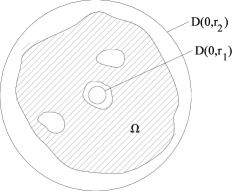
Figure 3.

Proof. Let $A$ be the annulus $D(0,r_{2})\setminus D(0,r_{1})$. Write $|df|$ for the euclidean norm of the euclidean gradient of $f$. Let $\rho$ be the function equal to $|df|$ on $\Omega$ and $0$ on ${\mathbb{C}\,}\setminus\Omega$. Then

$$\iint_{A}\rho^{2}dxdy = \iint_{\Omega}||\nabla_{g}f||_{g}^{2}d\mu_{g}\quad\mbox{ by conformal invariance of the energy}$$

$$\leq \sqrt{2}\iint_{\Omega}\langle\frac{\nabla_{g}f}{W},\nabla_{g}f\rangle_{g}d\mu_{g}\quad\mbox{ because $W\leq\sqrt{2}$ by point (5)}$$

$$= \sqrt{2}\iint_{\Omega}\mbox{\rm\,div\,}_{g}(f\frac{\nabla_{g}f}{W})d\mu_{g}\quad\mbox{ by the minimal surface equation \eqref{mse}}$$

$$= \sqrt{2}\int_{\partial\Omega}\frac{f}{W}\langle\nabla_{g}f,\nu_{g}\rangle_{g}ds_{g}\quad\mbox{ by the divergence theorem}$$

$$= \sqrt{2}\int_{\partial\Omega}\frac{f}{W}\langle\nabla f,\nu\rangle\quad\mbox{ where now all quantities are euclidean}$$

$$= \sqrt{2}\sum_{i=1}^{n}\int_{\gamma_{i}}\frac{f}{W}\langle\nabla f,\nu\rangle\quad\mbox{ by point (1)}$$

$$\leq -2\sqrt{2}h\sum_{i=1}^{n}\int_{\gamma_{i}}\frac{\langle\nabla f,\nu\rangle}{W}\quad\mbox{ by points (3) and (4)}$$

Hence by homology invariance of the flux,

(45) $$\iint_{A}\rho^{2}dxdy\leq 2\sqrt{2}h\phi$$

Consider the ray from $r_{1}e^{i\theta}$ to $r_{2}e^{i\theta}$. The integral of $df$ along this ray, intersected with $\Omega$, is equal to $h$. (If the ray happens to enter one of the disks $D_{i}$, then this is true because $f$ is constant on $\partial D_{i}$.) Integrating for $\theta\in[0,2\pi]$ we get

$$2\pi h \leq \int_{r=r_{1}}^{r_{2}}\int_{\theta=0}^{2\pi}\rho dr\,d\theta$$

$$= \int_{A}\frac{\rho}{r}dx\,dy$$

$$\leq \left(\iint_{A}\rho^{2}dx\,dy\right)^{1/2}\left(\iint_{A}\frac{1}{r^{2}}dx\,dy\right)^{1/2}\quad\mbox{ by Cauchy Schwartz}$$

$$\leq \left(2\sqrt{2}h\phi\right)^{1/2}\left(2\pi\log\frac{r_{2}}{r_{1}}\right)^{1/2}\quad\mbox{ using \eqref{eqq1}}$$

The proposition follows. $\Box$

The next proposition is useful to find circles on which we have a good estimate of $\int|df|$.

Proposition 20.

Under the same hypotheses as Proposition 19, consider some point $p\in\Omega$. Given $0<r^{\prime}_{1}<r^{\prime}_{2}$, there exists $r\in[r^{\prime}_{1},r^{\prime}_{2}]$ such that

$$\int_{C(p,r)\cap\Omega}|df|\leq\sqrt{8}\phi\left(\log\frac{r_{2}}{r_{1}}\right)^{1/2}\left(\log\frac{r^{\prime}_{2}}{r^{\prime}_{1}}\right)^{-1/2}.$$

Proof: Consider the function

$$F(r)=\int_{C(p,r)\cap\Omega}|df|=\int_{\theta=0}^{2\pi}\rho(p+re^{i\theta})rd\theta.$$

Then

$$\min_{r^{\prime}_{1}\leq r\leq r^{\prime}_{2}}F(r)\log\frac{r^{\prime}_{2}}{r^{\prime}_{1}}$$

$$\leq \int_{r=r^{\prime}_{1}}^{r^{\prime}_{2}}\frac{F(r)}{r}dr$$

$$= \int_{r=r^{\prime}_{1}}^{r^{\prime}_{2}}\int_{\theta=0}^{2\pi}\frac{\rho(p+re^{i\theta})}{r}rdrd\theta$$

$$\leq \left(\int_{r^{\prime}_{1}}^{r^{\prime}_{2}}\int_{0}^{2\pi}\rho(p+re^{i\theta})^{2}rdrd\theta\right)^{1/2}\left(\int_{r^{\prime}_{1}}^{r^{\prime}_{2}}\int_{0}^{2\pi}\frac{1}{r^{2}}rdrd\theta\right)^{1/2}$$

$$\leq \left(\int_{A}\rho^{2}dxdy\right)^{1/2}\left(2\pi\log\frac{r^{\prime}_{2}}{r^{\prime}_{1}}\right)^{1/2}$$

$$\leq \left(8\phi^{2}\log\frac{r_{2}}{r_{1}}\log\frac{r^{\prime}_{2}}{r^{\prime}_{1}}\right)^{1/2}\quad\mbox{ using \eqref{eqq1} and Proposition \ref{proposition-height}}$$

The proposition follows. $\Box$

A.5. A Laurent-type formula for $C^{1}$ functions

Proposition 21.

Let $\Omega\subset{\mathbb{C}\,}$ be a domain of the form

$$\Omega=D(0,R)\setminus\bigcup_{i=1}^{n}\overline{D}(p_{i},r_{i}).$$

Here we assume that the closed disks $\overline{D}(p_{i},r_{i})$ are disjoint and are included in $D(0,R)$. Let $f$ be a $C^{1}$ function on $\overline{\Omega}$. Then in $\Omega$,

$$f(z)=f^{+}(z)+\sum_{i=1}^{n}f^{-}_{i}(z)+\frac{1}{2\pi i}\int_{\Omega}\frac{f_{\overline{z}}(w)}{w-z}dw\wedge\overline{dw}$$

where $f^{+}$ is holomorphic in $D(0,R)$ and each $f^{-}_{i}$ is holomorphic in ${\mathbb{C}\,}\setminus\overline{D}(p_{i},r_{i})$. Moreover, these functions have the following series expansion

$$f^{+}(z)=\sum_{k=0}^{\infty}a_{k}z^{k}\qquad\mbox{ with }a_{k}=\frac{1}{2\pi i}\int_{C(0,R)}\frac{f(z)}{z^{k+1}}dz$$

$$f^{-}_{i}(z)=\sum_{k=1}^{\infty}\frac{a_{i,k}}{(z-p_{i})^{k}}\qquad\mbox{ with }a_{i,k}=\frac{1}{2\pi i}\int_{C(p_{i},r_{i})}f(z)(z-p_{i})^{k-1}dz$$

The series converge uniformly in compact subsets of $\Omega$.

Remark 11.

This is the same as the Laurent series theorem except that there is a correction term which vanishes when $f$ is holomorphic. The integration circles in the formula for $a_{n}$ and $a_{i,n}$ cannot be changed (as in the classical Laurent series theorem) since $f$ is not holomorphic.

Proof. By Cauchy Pompeieu integral formula for $C^{1}$ functions:

(46) $$f(z)=\frac{1}{2\pi i}\int_{\partial\Omega}\frac{f(w)}{w-z}dw+\frac{1}{2\pi i}\int_{\Omega}\frac{f_{\overline{z}}(w)}{w-z}dw\wedge\overline{dw}.$$

Define

$$f^{+}(z)=\frac{1}{2\pi i}\int_{C(0,R)}\frac{f(w)}{w-z}dw$$

$$f_{i}^{-}(z)=-\frac{1}{2\pi i}\int_{C(p_{i},r_{i})}\frac{f(w)}{w-z}dw$$

The function $f^{+}$ is holomorphic in $D(0,R)$. The function $f_{i}^{-}$ is holomorphic in ${\mathbb{C}\,}\setminus D(p_{i},r_{i})$ and extends at $\infty$ with $f_{i}^{-}(\infty)=0$. These two functions are expanded in power series exactly as in the proof of the classical theorem on Laurent series (see e.g. Conway [3] page 107). $\Box$

Proposition 22.

Let $\Omega\subset{\mathbb{C}\,}$ be a domain as in Proposition 21. Let $u:\Omega\to{\mathbb{R}}$ be a real-valued function of class $C^{2}$. Take $f=\partial u/\partial z$. Then the coefficients $a_{i,1}$ which appear in the conclusion of Proposition 21 are real.

Proof.

$$\mbox{\rm\,Im\,}a_{i,1} =\frac{-1}{2\pi}\mbox{\rm\,Re\,}\int_{C(p_{i},r_{i})}u_{z}dz$$

$$=\frac{-1}{4\pi}\int_{C(p_{i},r_{i})}u_{z}dz+u_{\overline{z}}d\overline{z}\quad\mbox{ because $u$ is real valued}$$

$$=\frac{-1}{4\pi}\int_{C(p_{i},r_{i})}du=0\quad\mbox{ because $u$ is well defined in $\Omega$}$$

∎

A.6. Residue computation

Proposition 23.

$$\mbox{\rm\,Res\,}_{p}(\log z-\log p)^{-1}=p,\qquad\mbox{\rm\,Res\,}_{p}(\frac{1-z^{2}}{4z^{2}})(\log z-\log p)^{-2}=-\frac{1+p^{2}}{4p}.$$

Proof.

$$\log z-\log p=\log\left(1+\frac{z-p}{p}\right)=\frac{z-p}{p}-\frac{1}{2}\left(\frac{z-p}{p}\right)^{2}+O(z-p)^{3}$$

The first residue follows. Then

$$(\log z-\log p)^{-2}=\left(\frac{z-p}{p}\right)^{-2}\left(1-\frac{1}{2}\left(\frac{z-p}{p}\right)\right)^{-2}=\frac{p^{2}}{(z-p)^{2}}+\frac{p}{z-p}+O(1).$$

Let

$$f(z)=\frac{1-z^{2}}{4z^{2}}=\frac{1}{4z^{2}}-\frac{1}{4}.$$

Then

$$\mbox{\rm\,Res\,}_{p}\left(\frac{1-z^{2}}{4z^{2}}(\log z-\log p)^{-2}\right) =\mbox{\rm\,Res\,}_{p}\left(\frac{f(z)p^{2}}{(z-p)^{2}}\right)+\mbox{\rm\,Res\,}_{p}\left(\frac{f(z)p}{(z-p)}\right)$$

$$=f^{\prime}(p)p^{2}+f(p)p\qquad(\text{by the Taylor expansion for $f$ at $p$})$$

$$=-\frac{1}{2p^{3}}p^{2}+\frac{1-p^{2}}{4p}$$

$$=-\frac{1+p^{2}}{4p}.$$

∎

References

- [1] S. Axler, P. Bourdon, W. Ramey: Harmonic Function Theory. Springer Verlag, New York (1992).
- [2] Alexander I. Bobenko: Helicoids with handles and Baker-Akhiezer spinors. Math. Z. 229:1, 9–29 (1998).
- [3] John B. Conway: Functions of One Complex Variable, Second Edition. Graduate Texts in Mathematics 11. Springer Verlag.
- [4] David Hoffman, Martin Traizet, Brian White: Helicoidal minimal surfaces of prescribed genus, I. Preprint (2013).
- [5] Rick Schoen: Uniqueness, Symmetry, and Embeddedness of Minimal Surfaces. J. of Differential Geometry 18, 791–809 (1983).
- [6] Markus Schmies: Computational methods for Riemann surfaces and helicoids with handles. Thesis, University of Berlin (2005).
- [7] Martin Traizet: A balancing condition for weak limits of minimal surfaces. Comment. Math. Helv. 79, 798–825 (2004).
- [8] Martin Traizet: On minimal surfaces bounded by two convex curves in parallel planes. Comment. Math. Helv. 85, 39–71 (2010).