A note on the CLT of the LSS for sample covariance matrix from a spiked population model

Abstract

In this note, we establish an asymptotic expansion for the centering parameter appearing in the central limit theorems for linear spectral statistic of large-dimensional sample covariance matrices when the population has a spiked covariance structure. As an application, we provide an asymptotic power function for the corrected likelihood ratio statistic for testing the presence of spike eigenvalues in the population covariance matrix. This result generalizes an existing formula from the literature where only one simple spike exists.

T1Research of this author was partly supported by the National Natural Science Foundation of China (Grant No. 11071213), the Natural Science Foundation of Zhejiang Province (No. R6090034), and the Doctoral Program Fund of Ministry of Education (No. J20110031). T2Research of this author was partly supported by the U.S. Army Research Office under Grant W911NF-09-1-0266. T3Research of this author was partly supported by a HKU start-up grant. and and

1 Introduction

Let $(\Sigma_{p})$ be a sequence of $p\times p$ non-random and nonnegative definite Hermitian matrices and let $(w_{ij})$, $i,j\geq 1$ be a doubly infinite array of i.i.d. complex-valued random variables satisfying

$$\;\mathbb{E}(w_{11})=0,\leavevmode\nobreak\ \leavevmode\nobreak\ \;\mathbb{E}(|w_{11}|^{2})=1,\leavevmode\nobreak\ \leavevmode\nobreak\ \;\mathbb{E}(|w_{11}|^{4})<\infty.$$

Write $Z_{n}=(w_{ij})_{1\leq i\leq p,1\leq j\leq n}$, the upper-left $p\times n$ block, where $p=p(n)$ is related to $n$ such that when $n\rightarrow\infty$, $p/n\rightarrow y>0$. Then the matrix $S_{n}=\frac{1}{n}\Sigma_{p}^{1/2}Z_{n}Z_{n}^{*}\Sigma_{p}^{1/2}$ can be considered as the sample covariance matrix of an i.i.d. sample $({\mathbf{x}}_{1},\ldots,{\mathbf{x}}_{n})$ of $p$-dimensional observation vectors ${\mathbf{x}}_{j}=\Sigma_{p}^{1/2}{{\mathbf{u}}_{j}}$ where ${{\mathbf{u}}_{j}}=(w_{ij})_{1\leq i\leq p}$ denotes the $j$-th column of $Z_{n}$. Note that for any nonnegative definite Hermitian matrix $A$, $A^{1/2}$ denotes a Hermitian square root and we call the spectral distribution (SD) the distribution generated by its eigenvalues.

Assume that the SD $H_{n}$ of $\Sigma_{p}$ converges weakly to a nonrandom probability distribution $H$ on $[0,\infty)$. It is then well-known that the SD $F^{S_{n}}$ of $S_{n}$, generated by its eigenvalues $\lambda_{n,1}\geq\cdots\geq\lambda_{n,p}$, converges to a nonrandom limiting SD $G$ (Marčenko and Pastur, 1967; Silverstein, 1995). The so-called null case corresponds to the situation $\Sigma_{p}\equiv I_{p}$, so $H_{n}\equiv\delta_{1}$ and the limiting SD is the seminal Marčenko-Pastur law $G^{y}$ with index $y$ and support $[a_{y},b_{y}]$ where $a_{y}=(1-\sqrt{y})^{2}$, $b_{y}=(1+\sqrt{y})^{2}$, and an additional mass at the origin if $y>1$.

In this paper we consider the spiked population model introduced in Johnstone (2001) where the eigenvalues of $\Sigma_{p}$ are

$$\underbrace{a_{1},\cdots,a_{1}}_{n_{1}},\ldots,\underbrace{a_{k},\cdots,a_{k}}_{n_{k}},\underbrace{1,\cdots,1}_{p-M}.$$ (1.1)

Here $M$ and the multiplicity numbers $(n_{k})$ are fixed and satisfy $n_{1}+\cdots+n_{k}=M$. In other words, all the population eigenvalues are unit except some fixed number of them (the spikes). The model can be viewed as a finite-rank perturbation of the null case. Obviously, the limiting SD $G$ of $S_{n}$ is not affected by this perturbation. However, the asymptotic behaviour of the extreme eigenvalues of $S_{n}$ is significantly different from the null case. The analysis of this new behaviour of extreme eigenvalues has been an active area in the last few years, see e.g. Baik et al. (2005), Baik and Silverstein (2006), Paul (2007), Bai and Yao (2008), Benaych-Georges et al. (2011), Nadakuditi and Silverstein (2010), Benaych-Georges and Nadakuditi (2011) and Bai and Yao (2012). In particular, the base component of the population SD $H_{n}$ in the last three references has been extended to a form more general than the simple Dirac mass $\delta_{1}$ of the null case.

For statistical applications, besides the principal components analysis which is indeed the origin of spiked models (Johnstone (2001)), large-dimensional strict factor models are equivalent to a spiked population model and can be analyzed using the above-mentioned results. Related recent contributions in the area include, among others, Kritchman and Nadler (2008, 2009), Onatski (2009, 2010, 2012) and Passemier and Yao (2012) and they all concern the problem of estimation and testing the number of factors (or spikes).

In this note, we analyze the effects caused by the spike eigenvalues on the fluctuations of linear spectral statistics of the form

$$T_{n}(f)=\sum_{i=1}^{p}f(\lambda_{n,i})=F^{S_{n}}(f)\leavevmode\nobreak\ ,$$ (1.2)

where $f$ is a given function. Similarly to the convergence of the SD’s, the presence of the spikes does not prevent a central limit theorem for $T_{n}(f)$; however as we will see, the centering term in the CLT will be modified according to the values of the spikes. As this term has no explicit form, our main result is an asymptotic expansion presented in Section 2. To illustrate the importance of such expansions, we present in Section 3 an application for the determination of the power function for testing the presence of spikes. The Appendix contains some technical derivations.

2 Centering parameter in the CLT of the LSS from a spiked population model

Fluctuations of linear spectral statistics of form (1.2) are indeed covered by a central limit theory initiated in Bai and Silverstein (2004). The theory was later improved by Pan and Zhou (2008) where the restriction $E(|w_{11}|^{4})=3$ matching the real Gaussian case was removed.

Let $f_{1},\ldots,f_{L}$ be $L$ functions analytic on an open domain of the complex plan including the support of the limiting SD. These central limit theorems state that the random vector

$$(X_{n}(f_{1}),\cdots,X_{n}(f_{L}))\leavevmode\nobreak\ ,$$

where

$$X_{n}(f)=p\left[F^{S_{n}}(f)-F^{y_{n},H_{n}}(f)\right]=p\int f(x)d(F^{S_{n}}-F^{y_{n},H_{n}})(x)\leavevmode\nobreak\ ,$$

converges weakly to a Gaussian vector

$$(X_{f_{1}},\cdots,X_{f_{L}})$$

with known mean function $E[X_{f}]$ and covariance function $Cov(X_{f},X_{g})$ that can be calculated from contour integrals involving parameters $\underline{m}(z)$ and $H$, where $\underline{m}(z)$ is the companion Stieltjes transform corresponding to the limiting SD of $\underline{S}_{n}=\frac{1}{n}Z_{n}^{*}\Sigma_{p}Z_{n}$. If the population has a spiked covariance structure, we know that the limit $H$ and $\underline{m}(z)$ remain the same as the non-spiked case, so the limiting parameters $E[X_{f}]$ and $Cov(X_{f},X_{g})$ are also unchanged.

It is remarked that the centering parameter $pF^{y_{n},H_{n}}(f)$ depends on a particular distribution $F^{y_{n},H_{n}}$ which is a finite-horizon proxy for the limiting SD of $S_{n}$. The difficulty is that $F^{y_{n},H_{n}}$ has no explicit form; it is indeed implicitly defined through $\underline{m}_{n}(z)$ (the finite counterpart of $\underline{m}(z)$), which solves the equation:

$$z=-\frac{1}{\underline{m}_{n}}+y_{n}\int\frac{t}{1+t\underline{m}_{n}}dH_{n}(t)\leavevmode\nobreak\ .$$ (2.3)

This distribution depends on the SD $H_{n}$ which in turn depends on the spike eigenvalues.

More precisely, the SD $H_{n}$ of $\Sigma_{p}$ is

$$H_{n}=\frac{p-M}{p}\delta_{1}+\frac{1}{p}\sum_{i=1}^{k}n_{i}\delta_{a_{i}}\leavevmode\nobreak\ .$$ (2.4)

The term

$$\frac{1}{p}\sum_{i=1}^{k}n_{i}\delta_{a_{i}}$$

vanishes when $p$ tends to infinity, so it has no influence when considering limiting spectral distributions. However for the CLT, the term $pF^{y_{n},H_{n}}(f)$ has a $p$ in front, and $\frac{1}{p}\sum_{i=1}^{k}n_{i}\delta_{a_{i}}$ times $p$ is of order $O(1)$, thus cannot be neglected.

It is here reminded that, following Baik and Silverstein (2006), for a distant spike $a_{i}$ such that $|a_{i}-1|>\sqrt{y}$, the corresponding sample eigenvalue is equal to $\phi(a_{i})=a_{i}+\frac{ya_{i}}{a_{i}-1}$, while for a close spike such that $|a_{i}-1|\leq\sqrt{y}$, the corresponding sample eigenvalue tends to the edge points $a_{y}$ and $b_{y}$.

Our main result is an asymptotic expansion for this centering parameter.

Theorem 1.

Suppose the population has a spiked population structure as stated in (1.1) with $k_{1}$ distant spikes and $k-k_{1}$ close spikes (arranged in decreasing order), Let $f$ be any analytic function on an open domain including the support of M-P distribution $G^{y}$ and all the $\phi(a_{i})$, $i\leq k_{1}$. We have:

$$F^{y_{n},H_{n}}(f)$$

$$= -\frac{1}{2\pi ip}\oint_{\mathcal{C}_{1}}f(-\frac{1}{\underline{m}}+\frac{y_{n}}{1+\underline{m}})(\frac{M}{y_{n}\underline{m}}-\sum_{i=1}^{k}\frac{n_{i}a_{i}^{2}\underline{m}}{(1+a_{i}\underline{m})^{2}})d\underline{m}$$ (2.5)

$$+ \frac{1}{2\pi ip}\oint_{\mathcal{C}_{1}}f^{{}^{\prime}}(-\frac{1}{\underline{m}}+\frac{y_{n}}{1+\underline{m}})\sum_{i=1}^{k}\frac{(1-a_{i})n_{i}}{(1+a_{i}\underline{m})(1+\underline{m})}(\frac{1}{\underline{m}}-\frac{y_{n}\underline{m}}{(1+\underline{m})^{2}})d\underline{m}$$ (2.6)

$$+ (1-\frac{M}{p})G^{y_{n}}(f)+\frac{1}{p}\sum_{i=1}^{k_{1}}n_{i}f(\phi(a_{i}))+O(\frac{1}{n^{2}})\leavevmode\nobreak\ ;$$ (2.7)

Here $\underline{m}=\underline{m}_{n}$ is the companion Stieltjes transform of $F^{y_{n},H_{n}}$ defined in (2.3), $G^{y_{n}}(f)$ is the integral of $f$ with respect to the Marčenko-Pastur distribution with index $y_{n}=p/n$. And

1. when $0<y_{n}<1$, the first $k_{1}$ spike eigenvalues $a_{i}^{\prime}s$ satisfy $|a_{i}-1|>\sqrt{y_{n}}$, the remaining $k-k_{1}$ satisfy $|a_{i}-1|\leq\sqrt{y_{n}}$, $\mathcal{C}_{1}$ is a contour counterclockwise, when restricted to the real axes, encloses the interval $[\frac{-1}{1-\sqrt{y_{n}}},\frac{-1}{1+\sqrt{y_{n}}}]$;

2. when $y_{n}\geq 1$, the first $k_{1}$ spike eigenvalues $a_{i}^{\prime}s$ satisfy $a_{i}-1>\sqrt{y_{n}}$, the remaining $k-k_{1}$ satisfy $0<a_{i}\leq 1+\sqrt{y_{n}}$, $\mathcal{C}_{1}$ is a contour clockwise, when restricted to the real axes, encloses the interval $[-1,\frac{-1}{1+\sqrt{y_{n}}}]$.

If there are no distant spikes then the second term in (2.7) does not appear.

Proof.

We divide the proof into three parts according to whether $0<y_{n}<1$, $y_{n}>1$ or $y_{n}=1$.

Case of $0<y_{n}<1$:

Recall that $G^{y_{n}}(f)=\int f(x)dG^{y_{n}}(x)$ when no spike exists, where $G^{y_{n}}$ is the M-P distribution with index $y_{n}$. And by the Cauchy integral formula, it can be expressed as $-\frac{1}{2\pi i}\oint_{\gamma_{1}}f(z)m(z)dz$, where the integral contour $\gamma_{1}$ is chosen to be positively oriented, enclosing the support of $G^{y_{n}}$ and it’s limit $G^{y}$. Due to the restriction that $0<y_{n}<1$, we choose $\gamma_{1}$ such that the origin $\{z=0\}$ is not enclosed inside.

Using the relationship between $m(z)$ and $\underline{m}(z)$ (the companion Stieltjes transform of $m(z)$):  $\underline{m}(z)=y_{n}m(z)-\frac{1-y_{n}}{z}$, we can rewrite

$$G^{y_{n}}(f) = -\frac{1}{2\pi i}\oint_{\gamma_{1}}f(z)m(z)dz=-\frac{1}{2\pi i}\oint_{\gamma_{1}}f(z)\Big{(}\frac{\underline{m}(z)}{y_{n}}+\frac{1-y_{n}}{y_{n}z}\Big{)}dz$$ (2.8)

$$= -\frac{n}{p}\frac{1}{2\pi i}\oint_{\gamma_{1}}f(z)\underline{m}(z)dz\leavevmode\nobreak\ .$$

Besides, for $z\notin supp(G^{y_{n}})$, $\underline{m}(z)$ satisfies the equation:

$$z=-\frac{1}{\underline{m}}+\frac{y_{n}}{1+\underline{m}}\leavevmode\nobreak\ .$$ (2.9)

Taking derivatives on both sides with respect to $z$, we get:

$$dz=(\frac{1}{\underline{m}^{2}}-\frac{y_{n}}{(1+\underline{m})^{2}})d\underline{m}\leavevmode\nobreak\ .$$

Changing the variable from $z$ to $\underline{m}$ in equation (2.8), we get:

$$G^{y_{n}}(f)=-\frac{n}{p}\frac{1}{2\pi i}\oint_{\mathcal{C}_{1}}f(-\frac{1}{\underline{m}}+\frac{y_{n}}{1+\underline{m}})\underline{m}(z)(\frac{1}{\underline{m}^{2}}-\frac{y_{n}}{(1+\underline{m})^{2}})d\underline{m}\leavevmode\nobreak\ .$$ (2.10)

Here, the contour $\gamma_{1}$ of $z$ in equation (2.8) is transformed into a contour of $\underline{m}$ through the mapping (2.9), denoted as $\mathcal{C}_{1}$.

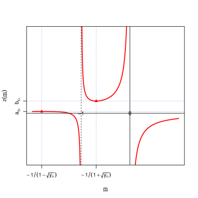
We present the mapping (2.9) when $0<y_{n}<1$ in Figure 1, restricting $z$ and $\underline{m}$ to the real domain. From Silverstein and Choi (1995), we know that the $z^{\prime}s$ such that $z^{{}^{\prime}}(m)>0$ are not in the support of $G^{y_{n}}$. Therefore, we shall focus on the increasing intervals, where a one-to-one mapping between $z$ and $\underline{m}$ exists. From the figure, we see that when $\gamma_{1}$ is chosen to enclose the support of ${\color[rgb]{0,0,0}G^{y_{n}}}$: $[a_{y_{n}},b_{y_{n}}]$, the corresponding $\mathcal{C}_{1}$ will enclose the interval $[\frac{-1}{1-\sqrt{y_{n}}},\frac{-1}{1+\sqrt{y_{n}}}]$, and $\underline{m}=-1$ is the pole contained in this interval. The point on $\gamma_{1}$ intersecting the real line to the left of $a_{y_{n}}$ (right of $b_{y_{n}}$) maps to a point to the left of $\frac{-1}{1-\sqrt{y_{n}}}$ (right of $\frac{-1}{1+\sqrt{y_{n}}}$). Since the imaginary part of $\underline{m}(z)$ is the same sign as the imaginary part of $z$, we see that $\mathcal{C}_{1}$ is also oriented counterclockwise.

Figure 1: The graph of the transform $z(\underline{m})=-\frac{1}{\underline{m}}+\frac{y_{n}}{1+\underline{m}}$ when $0<y_{n}<1$.

When the spiked structure (1.1) exists, by equation (2.3), this time the companion Stieltjes transform $\underline{m}=\underline{m}_{n}$ of $F^{y_{n},H_{n}}$ satisfies

$$z=-\frac{1}{\underline{m}}+\frac{p-M}{p}\frac{y_{n}}{1+\underline{m}}+\frac{y_{n}}{p}\sum_{i=1}^{k}\frac{a_{i}n_{i}}{1+a_{i}\underline{m}}\leavevmode\nobreak\ ,$$ (2.11)

$$dz=\bigg{(}\frac{1}{\underline{m}^{2}}-\frac{p-M}{p}\frac{y_{n}}{(1+\underline{m})^{2}}-\frac{y_{n}}{p}\sum_{i=1}^{k}\frac{a_{i}^{2}n_{i}}{(1+a_{i}\underline{m})^{2}}\bigg{)}d\underline{m}\leavevmode\nobreak\ .$$

Repeating the same computation as before, we get:

$$F^{y_{n},H_{n}}(f)=-\frac{n}{p}\frac{1}{2\pi i}\oint_{\gamma}f(z)\underline{m}(z)dz$$ (2.12)

$$= -\frac{n}{p}\frac{1}{2\pi i}\oint_{\mathcal{C}}f\bigg{(}-\frac{1}{\underline{m}}+\frac{y_{n}}{1+\underline{m}}-\frac{y_{n}}{p}\sum_{i=1}^{k}\frac{(1-a_{i})n_{i}}{(1+\underline{m})(1+a_{i}\underline{m})}\bigg{)}\underline{m}$$

$$\times\bigg{(}\frac{1}{\underline{m}^{2}}-\frac{y_{n}}{(1+\underline{m})^{2}}+\frac{y_{n}}{p}\sum_{i=1}^{k}n_{i}\bigg{[}\frac{1}{(1+\underline{m})^{2}}-\frac{a_{i}^{2}}{(1+a_{i}\underline{m})^{2}}\bigg{]}\bigg{)}d\underline{m},$$

where $\gamma$ is a positively oriented contour of $z$ that encloses the support of $F^{S_{n}}$ and its limit $F^{S}$. From Baik and Silverstein (2006), we know that under the spiked structure (1.1), the support of $F^{S_{n}}$ consists of the support of M-P distribution: $[a_{y_{n}},b_{y_{n}}]$ plus small intervals near $\phi(a_{i})=a_{i}+\frac{y_{n}a_{i}}{a_{i}-1}$ $(i=1,\cdots,k_{1})$. Therefore, the contour $\gamma$ can be expressed as $\gamma_{1}\bigoplus(\bigoplus_{i=1}^{k_{1}}\gamma_{a_{i}})$ ($\gamma_{a_{i}}$ is denoted as the contour that encloses the point of $\phi(a_{i})$). Moreover, $\mathcal{C}$ is the image of $\gamma$ under the mapping (2.11), which can also be divided into $\mathcal{C}_{1}$ plus $\mathcal{C}_{a_{i}}$ $(i=1,\cdots,k_{1})$, with $\mathcal{C}_{a_{i}}$ enclosing $-\frac{1}{a_{i}}$ and all the contours are non-overlapping and positively oriented.

The term

$$\frac{y_{n}}{p}\sum_{i=1}^{k}\frac{(1-a_{i})n_{i}}{(1+\underline{m})(1+a_{i}\underline{m})}$$

is of order $O(\frac{1}{n})$, so we can take the Taylor expansion of $f$ around the value of $-\frac{1}{\underline{m}}+\frac{y_{n}}{1+\underline{m}}$, and the term

$$\frac{y_{n}}{p}\sum_{i=1}^{k}n_{i}\bigg{[}\frac{1}{(1+\underline{m})^{2}}-\frac{a_{i}^{2}}{(1+a_{i}\underline{m})^{2}}\bigg{]}$$

is also of order $O(\frac{1}{n})$. This gives rise to:

$$F^{y_{n},H_{n}}(f)=-\frac{n}{p}\frac{1}{2\pi i}\oint_{\mathcal{C}}f(-\frac{1}{\underline{m}}+\frac{y_{n}}{1+\underline{m}})(\frac{1}{\underline{m}}-\frac{y_{n}\underline{m}}{(1+\underline{m})^{2}})d\underline{m}$$

$$-\frac{n}{p}\frac{1}{2\pi i}\oint_{\mathcal{C}}f(-\frac{1}{\underline{m}}+\frac{y_{n}}{1+\underline{m}})\frac{y_{n}}{p}\sum_{i=1}^{k}n_{i}\bigg{[}\frac{1}{(1+\underline{m})^{2}}-\frac{a_{i}^{2}}{(1+a_{i}\underline{m})^{2}}\bigg{]}\underline{m}d\underline{m}$$

$$+\frac{n}{p}\frac{1}{2\pi i}\oint_{\mathcal{C}}f^{{}^{\prime}}(-\frac{1}{\underline{m}}+\frac{y_{n}}{1+\underline{m}})\frac{y_{n}}{p}\sum_{i=1}^{k}\frac{(1-a_{i})n_{i}}{(1+\underline{m})(1+a_{i}\underline{m})}(\frac{1}{\underline{m}}-\frac{y_{n}\underline{m}}{(1+\underline{m})^{2}})d\underline{m}$$

$$+O(\frac{1}{n^{2}})\leavevmode\nobreak\ .$$ (2.13)

Then, we replace $\mathcal{C}$ appearing in equation (2) by $\mathcal{C}_{1}\bigoplus(\bigoplus_{i=1}^{k_{1}}\mathcal{C}_{a_{i}})$ as mentioned above, and thus we can calculate the value of (2) separately by calculating the integrals on the contour $\mathcal{C}_{1}$ and each $\mathcal{C}_{a_{i}}$ $(i=1,\cdots,k_{1})$. If there are no distant spikes then we will have just $\mathcal{C}=\mathcal{C}_{1}$.

The first term in equation (2) is equal to

$$-\frac{n}{p}\frac{1}{2\pi i}\oint_{\mathcal{C}_{1}}f(-\frac{1}{\underline{m}}+\frac{y_{n}}{1+\underline{m}})(\frac{1}{\underline{m}}-\frac{y_{n}\underline{m}}{(1+\underline{m})^{2}})d\underline{m}$$ (2.14)

for the reason that the only poles: $\underline{m}=0$ and $\underline{m}=-1$ are not enclosed in the contours $C_{a_{i}}$ $(i=1,\cdots,k_{1})$.

Next, we consider these integrals on $\mathcal{C}_{a_{i}}(i=1,\cdots,k_{1})$.

The second term of equation (2) with the contour being $\mathcal{C}_{a_{i}}$ is equal to

$$-\frac{n}{p}\frac{1}{2\pi i}\oint_{\mathcal{C}_{a_{i}}}f(-\frac{1}{\underline{m}}+\frac{y_{n}}{1+\underline{m}})\frac{y_{n}}{p}\sum_{i=1}^{k}n_{i}\bigg{[}\frac{1}{(1+\underline{m})^{2}}-\frac{a_{i}^{2}}{(1+a_{i}\underline{m})^{2}}\bigg{]}\underline{m}d\underline{m}$$

$$= \frac{n}{p}\frac{1}{2\pi in}\oint_{\mathcal{C}_{a_{i}}}f(-\frac{1}{\underline{m}}+\frac{y_{n}}{1+\underline{m}})\sum_{i=1}^{k}\frac{a_{i}^{2}n_{i}\underline{m}}{(1+a_{i}\underline{m})^{2}}d\underline{m}$$

$$= \frac{1}{2\pi ip}\oint_{\mathcal{C}_{a_{i}}}\frac{f(-\frac{1}{\underline{m}}+\frac{y_{n}}{1+\underline{m}})\underline{m}n_{i}}{(\underline{m}+\frac{1}{a_{i}})^{2}}d\underline{m}$$

$$= \frac{n_{i}}{p}\Big{[}f(\phi(a_{i}))-f^{{}^{\prime}}(\phi(a_{i}))\Big{(}a_{i}-\frac{y_{n}a_{i}}{(a_{i}-1)^{2}}\Big{)}\Big{]}\leavevmode\nobreak\ ,$$

and the third term of equation (2) with the contour being $\mathcal{C}_{a_{i}}$ is equal to

$$\frac{n}{p}\frac{1}{2\pi i}\oint_{\mathcal{C}_{a_{i}}}f^{{}^{\prime}}(-\frac{1}{\underline{m}}+\frac{y_{n}}{1+\underline{m}})\frac{y_{n}}{p}\sum_{i=1}^{k}\frac{(1-a_{i})n_{i}}{(1+\underline{m})(1+a_{i}\underline{m})}(\frac{1}{\underline{m}}-\frac{y_{n}\underline{m}}{(1+\underline{m})^{2}})d\underline{m}$$

$$= \frac{-1}{2\pi ip}\oint_{\mathcal{C}_{a_{i}}}f^{{}^{\prime}}(-\frac{1}{\underline{m}}+\frac{y_{n}}{1+\underline{m}})\frac{n_{i}(1-a_{i})}{(\underline{m}+\frac{1}{a_{i}})a_{i}(\underline{m}+1)}(\frac{1}{\underline{m}}-\frac{y_{n}\underline{m}}{(1+\underline{m})^{2}})d\underline{m}$$

$$= \frac{1}{p}n_{i}f^{{}^{\prime}}(\phi(a_{i}))\Big{(}a_{i}-\frac{y_{n}a_{i}}{(a_{i}-1)^{2}}\Big{)}\leavevmode\nobreak\ .$$

Combining these two terms, we get the influence of the distant spikes, that is, the integral on the contours $\bigcup_{i=1,\cdots,k_{1}}\mathcal{C}_{a_{i}}$, which equals to:

$$\frac{1}{p}\sum_{i=1}^{k_{1}}n_{i}f(\phi(a_{i}))\leavevmode\nobreak\ .$$ (2.15)

So in the remaining part, we only need to consider the integral along the contour $\mathcal{C}_{1}$. Consider the second term of (2) with the contour being $\mathcal{C}_{1}$:

$$-\frac{n}{p}\frac{1}{2\pi i}\oint_{\mathcal{C}_{1}}f(-\frac{1}{\underline{m}}+\frac{y_{n}}{1+\underline{m}})\frac{y_{n}}{p}\sum_{i=1}^{k}n_{i}\bigg{[}\frac{1}{(1+\underline{m})^{2}}-\frac{a_{i}^{2}}{(1+a_{i}\underline{m})^{2}}\bigg{]}\underline{m}d\underline{m}$$ (2.16)

$$= -\frac{1}{2\pi ip}\oint_{\mathcal{C}_{1}}f(-\frac{1}{\underline{m}}+\frac{y_{n}}{1+\underline{m}})\bigg{[}\frac{1}{y_{n}}(\frac{M\underline{m}y_{n}}{(1+\underline{m})^{2}}-\frac{M}{\underline{m}})+\frac{1}{y_{n}}\frac{M}{\underline{m}}-\sum_{i=1}^{k}\frac{n_{i}a_{i}^{2}\underline{m}}{(1+a_{i}\underline{m})^{2}}\bigg{]}d\underline{m}$$

$$= -\frac{M}{p}\frac{n}{2\pi ip}\oint_{\mathcal{C}_{1}}f(-\frac{1}{\underline{m}}+\frac{y_{n}}{1+\underline{m}})\big{(}\frac{\underline{m}y_{n}}{(1+\underline{m})^{2}}-\frac{1}{\underline{m}}\big{)}d\underline{m}$$

$$-\frac{1}{2\pi ip}\oint_{\mathcal{C}_{1}}f(-\frac{1}{\underline{m}}+\frac{y_{n}}{1+\underline{m}})\bigg{(}\frac{M}{\underline{m}y_{n}}-\sum_{i=1}^{k}\frac{n_{i}a_{i}^{2}\underline{m}}{(1+a_{i}\underline{m})^{2}}\bigg{)}d\underline{m}\leavevmode\nobreak\ .$$

Combining Equations (2.10), (2.14), (2.15) and (2.16), we get:

$$F^{y_{n},H_{n}}(f)=-\frac{1}{2\pi ip}\oint_{\mathcal{C}_{1}}f(-\frac{1}{\underline{m}}+\frac{y_{n}}{1+\underline{m}})(\frac{M}{\underline{m}y_{n}}-\sum_{i=1}^{k}\frac{n_{i}a_{i}^{2}\underline{m}}{(1+a_{i}\underline{m})^{2}})d\underline{m}$$

$$+\frac{1}{2\pi ip}\oint_{\mathcal{C}_{1}}f^{{}^{\prime}}(-\frac{1}{\underline{m}}+\frac{y_{n}}{1+\underline{m}})\sum_{i=1}^{k}\frac{(1-a_{i})n_{i}}{(1+\underline{m})(1+a_{i}\underline{m})}(\frac{1}{\underline{m}}-\frac{y_{n}\underline{m}}{(1+\underline{m})^{2}})d\underline{m}$$

$$+(1-\frac{M}{p})G^{y_{n}}(f)+\sum_{i=1}^{k_{1}}\frac{n_{i}}{p}f(\phi(a_{i}))+O(\frac{1}{n^{2}})\leavevmode\nobreak\ .$$

Case of $y_{n}>1$:

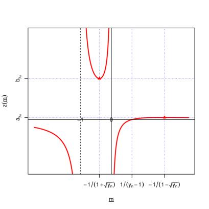
We also present the mapping (2.9) when $y_{n}>1$ in Figure 2 below.

Figure 2: The graph of the transform $z(\underline{m})=-\frac{1}{\underline{m}}+\frac{y_{n}}{1+\underline{m}}$ when $y_{n}>1$.

When $y_{n}>1$ there will be mass $1-1/y_{n}$ at zero. Assume first that $f$ is analytic on an open interval containing 0 and $b_{y_{n}}$ and let $\gamma_{1}$ be a contour covering $[a_{y_{n}},b_{y_{n}}]$. Then we have in place of (2.8),

$$G^{y_{n}}(f) = (1-\frac{1}{y_{n}})f(0)-\frac{1}{2\pi i}\oint_{\gamma_{1}}f(z)m(z)dz$$

$$= (1-\frac{1}{y_{n}})f(0)-\frac{1}{2\pi iy_{n}}\oint_{\gamma_{1}}f(z)\underline{m}(z)dz.$$

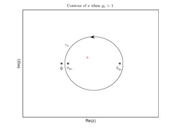
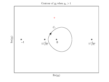
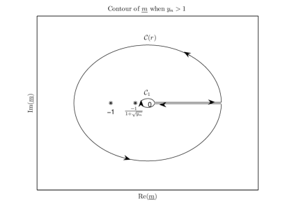
This time the $\underline{m}$ value corresponding to $a_{y_{n}}$, namely $\frac{-1}{1-\sqrt{y_{n}}}$, is positive, and so when changing variables the new contour $\mathcal{C}$ covers $[c_{n},d_{n}]$ where $c_{n}<0$ is slightly to the right of $\frac{-1}{1+\sqrt{y_{n}}}$, and $d_{n}>0$ is slightly to the left of $\frac{-1}{1-\sqrt{y_{n}}}$, This interval includes the origin and not $-1$, and is oriented in a clockwise direction. We present these two contours $\gamma_{1}$ and $\mathcal{C}_{1}$ in Figure 3.

Figure 3: Contours of $z$ and $\underline{m}$ when $y_{n}>1$.

We have in place of (2.10),

$$G_{y_{n}}(f)=(1-\frac{1}{y_{n}})f(0)-\frac{1}{2\pi iy_{n}}\oint_{{\color[rgb]{0,0,0}\mathcal{C}_{1}}}f(-\frac{1}{\underline{m}}+\frac{y_{n}}{1+\underline{m}})\underline{m}(\frac{1}{\underline{m}^{2}}-\frac{y_{n}}{(1+\underline{m})^{2}})d\underline{m}.$$

Extend $\mathcal{C}_{1}$ to the following contour. On the right side on the real line continue $\mathcal{C}_{1}$ to a number large number $r$, then go on a circle $\mathcal{C}(r)$ with radius $r$ in a counterclockwise direction until it returns to the point $r-i0$, then go left till it hits $\mathcal{C}_{1}$. This new contour covers pole $-1$ and not the origin, see Figure 4.

Figure 4: The new contour of $\underline{m}$ when $y_{n}>1$

On $\mathcal{C}(r)$ we have using the dominated convergence theorem

$$\frac{1}{2\pi iy_{n}}\oint_{\mathcal{C}(r)}f(-\frac{1}{\underline{m}}+\frac{y_{n}}{1+\underline{m}})\underline{m}(\frac{1}{\underline{m}^{2}}-\frac{y_{n}}{(1+\underline{m})^{2}})d\underline{m}$$

$$(\text{with }\underline{m}=re^{i\theta})$$

$$= \frac{1}{2\pi y_{n}}\int_{0}^{2\pi}f(-\frac{1}{\underline{m}}+\frac{y_{n}}{1+\underline{m}})(1-\frac{y_{n}\underline{m}^{2}}{(1+\underline{m})^{2}})d\theta$$

$$\to\quad\frac{1-y_{n}}{y_{n}}{\color[rgb]{0,0,0}f(0)}\quad(\text{as }r\to\infty).\quad$$

Therefore

$$G_{y_{n}}(f)=-\frac{n}{p}\frac{1}{2\pi i}\oint_{{\color[rgb]{0,0,0}\mathcal{C}_{1}}}f(-\frac{1}{\underline{m}}+\frac{y_{n}}{1+\underline{m}})\underline{m}(\frac{1}{\underline{m}^{2}}-\frac{y_{n}}{(1+\underline{m})^{2}})d\underline{m}.$$ (2.17)

where $\mathcal{C}_{1}$ just covers $[-1,\frac{-1}{1+\sqrt{y_{n}}}]$.

When there are spikes the only distant ones are those for which $a_{i}>1+\sqrt{y_{n}}$. We will get after the change of variable to $\underline{m}$ a contour which covers now $[c^{\prime}_{n},d^{\prime}_{n}]$ where $c^{\prime}_{n}<0$ is to the right of the largest of $-\frac{1}{a_{i}}$ among the distant spikes (to the right of $\frac{-1}{1+\sqrt{y_{n}}}$ if there are no distant spikes), and $d^{\prime}_{n}>0$ is to the left of $\frac{-1}{1-\sqrt{y_{n}}}$, and oriented clockwise. We can extend the contour as we did before and get the same limit on the circle as when there are no spikes. Therefore we get exactly (2.12) where now the contour $\mathcal{C}$ contains $-1$ and the largest of $-\frac{1}{a_{i}}$ among the distant spikes (contain $\frac{-1}{1+\sqrt{y_{n}}}$ if there are no distant spikes). Next, we can follow the same proof as for the case $0<y_{n}<1$, by slitting the contour $\mathcal{C}$ into $\mathcal{C}=\mathcal{C}_{1}\bigoplus(\bigoplus_{i=1}^{k_{1}}\mathcal{C}_{a_{i}})$, where now $\mathcal{C}_{1}$ just contains the interval $[-1,\frac{-1}{1+\sqrt{y_{n}}}]$ and the contours $\mathcal{C}_{a_{i}}$ contain the influence of $k_{1}$ distant spikes $a_{i}>1+\sqrt{y_{n}}$: $-\frac{1}{a_{i}}$ ($i=1,\cdots,k_{1}$), respectively. We thus obtain the same formula as in the case $0<y_{n}<1$. Therefore Theorem 1 follows where $\mathcal{C}_{1}$ contains just $[-1,\frac{-1}{1+\sqrt{y_{n}}}]$, and none of the $-\frac{1}{a_{i}}$ among the distant spikes ($-\frac{1}{a_{i}}$ are enclosed in the contour $\mathcal{C}_{a_{i}}$ as the case of $0<y_{n}<1$).

Case of $y_{n}=1$:

For $y_{n}=1$ we have $m(z)=\underline{m}(z)$, and the contour defining $G_{1}(f)$ must contain the interval $[0,4]$. The contour in $\underline{m}$ contains $[c_{n},d_{n}]$ where $-\frac{1}{2}<c_{n}<0$, $d_{n}>0$ and again is oriented in the clockwise direction. Extending again this contour we find the limit of the integral on the circle is zero for both $G_{1}(f)$ and $F^{1,H_{n}}(f)$, and we get again Theorem 1 where $\mathcal{C}_{1}$ is a contour containing $[-1,-\frac{1}{2}]$, and not the origin.

The proof of the theorem is complete. ∎

3 An application to the test of presence of spike eigenvalues

In Bai et al. (2009), a corrected likelihood ratio statistic $\tilde{L}^{*}$ is proposed to test the hypothesis

$$H_{0}:\leavevmode\nobreak\ \Sigma=I_{p}\leavevmode\nobreak\ \leavevmode\nobreak\ \leavevmode\nobreak\ vs.\leavevmode\nobreak\ \leavevmode\nobreak\ \leavevmode\nobreak\ H_{1}:\leavevmode\nobreak\ \Sigma\neq I_{p}\leavevmode\nobreak\ .$$

They prove that under $H_{0}$,

$$\tilde{L}^{*}-pG^{y_{n},H_{n}}(g)\Rightarrow N(m(g),v(g))\leavevmode\nobreak\ ,$$

where

$$\tilde{L}^{*}=trS_{n}-\log|S_{n}|-p\leavevmode\nobreak\ ,$$

$$G^{y_{n},H_{n}}(g)=1-\frac{y_{n}-1}{y_{n}}\log(1-y_{n})\leavevmode\nobreak\ ,$$

$$m(g)=-\frac{\log(1-y)}{2}\leavevmode\nobreak\ ,$$

$$v(g)=-2\log(1-y)-2y.$$

At a significance level $\alpha$ (usually 0.05), the test will reject $H_{0}$ when $\tilde{L}^{*}-pG^{y_{n},H_{n}}(g)>m(g)+\Phi^{-1}(1-\alpha)\sqrt{v(g)}$ where $\Phi$ is the standard normal cumulative distribution function.

However, the power function of this test remains unknown because the distribution of $\tilde{L}^{*}$ under the general alternative hypothesis $H_{1}$ is ill-defined. Let’s consider this general test as a way to test the null hypothese $H_{0}$ above against an alternative hypothesis of the form:

$$H_{1}^{*}:\leavevmode\nobreak\ \Sigma_{p}\textrm{ has the spiked structure \eqref{model}.}$$

In other words, we want to test the absence against the presence of possible spike eigenvalues in the population covariance matrix. The general asymptotic expansion in Theorem 1 helps to find the power function of the test.

More precisely, under the alternative $H_{1}^{*}$ and for $f(x)=x-\log x-1$ used in the statistic $\tilde{L}^{*}$, the centering term $F^{y_{n},H_{n}}(f)$ can be found to be

$$1+\frac{1}{p}\sum_{i=1}^{k}n_{i}a_{i}-\frac{M}{p}-\frac{1}{p}\sum_{i=1}^{k}n_{i}\log a_{i}-(1-\frac{1}{y_{n}})\log(1-y_{n})+O(\frac{1}{n^{2}})\leavevmode\nobreak\ ,$$

thanks to the following formulas

$$F^{y_{n},H_{n}}(x)=1+\frac{1}{p}\sum_{i=1}^{k}n_{i}a_{i}-\frac{M}{p}+O(\frac{1}{n^{2}})\leavevmode\nobreak\$$ (3.18)

and

$$F^{y_{n},H_{n}}(\log x)=\frac{1}{p}\sum_{i=1}^{k}n_{i}\log a_{i}-1+(1-\frac{1}{y_{n}})\log(1-y_{n})+O(\frac{1}{n^{2}})\leavevmode\nobreak\ .$$ (3.19)

The details of derivation of these formulas are given in the Appendix A.

Therefore we have obtained that under $H_{1}^{*}$,

$$\tilde{L}^{*}-pF^{y_{n},H_{n}}(f)\Rightarrow N(m(g),v(g))\leavevmode\nobreak\ .$$

It follows that the asymptotic power function of the test is

$$\beta(\alpha)=1-\Phi\Bigg{(}\Phi^{-1}(1-\alpha)-\frac{\sum_{i=1}^{k}n_{i}(a_{i}-1-\log a_{i})}{\sqrt{-2\log(1-y)-2y}}\Bigg{)}\leavevmode\nobreak\ .$$

In the particular case where the spiked model has only one simple close spike, i.e. $k=1$, $k_{1}=0$, $n_{1}=1$, the above power function becomes

$$\beta(\alpha)=1-\Phi\left(\Phi^{-1}(1-\alpha)-\frac{a_{1}-1-\log a_{1}}{\sqrt{-2\log(1-y)-2y}}\right)\leavevmode\nobreak\ ,$$

which is exactly the formula $(5.6)$ found in Onatski et al. (2011). Note that these authors have found this formula using a sophisticated tools of asymptotic contiguity and Le Cam’s first and third lemmas, our derivation is in a sense much more direct.

Appendix A Additional proofs of $\eqref{app1}$ and $\eqref{app2}$

The likelihood ratio test works only when $0<y_{n}<1$, and when $k_{1}+1\leq i\leq k$, the corresponding $a_{i}$ satisfy $|a_{i}-1|\leq\sqrt{y_{n}}$, which is equivalent to $-\frac{1}{a_{i}}\in[\frac{-1}{1-\sqrt{y_{n}}},\frac{-1}{1+\sqrt{y_{n}}}]$, so poles of $\{\underline{m}=-1\}$, $\{\underline{m}=-\frac{1}{a_{i}},i=(k_{1}+1,\cdots,k)\}$ and $\{\underline{m}=\frac{1}{y_{n}-1}\}$ (pole of the function $logz$) should be included in $\mathcal{C}_{1}$. In all the following, we write $m$ to stand for $\underline{m}$ for convenience.

A.1 Proof of $\eqref{app1}$

We have

$$\eqref{th1}=-\frac{1}{2\pi ip}\oint_{\mathcal{C}_{1}}(-\frac{1}{m}+\frac{y_{n}}{1+m})(\frac{M}{y_{n}m}-\sum_{i=1}^{k}\frac{n_{i}a_{i}^{2}m}{(1+a_{i}m)^{2}})dm\leavevmode\nobreak\ ,$$ (A.20)

and its residual at $m=-1$ equals to

$$\frac{M}{p}-\frac{y_{n}}{p}\sum_{i=1}^{k}\frac{n_{i}a_{i}^{2}}{(1-a_{i})^{2}}\leavevmode\nobreak\ .$$ (A.21)

$$\eqref{th2}=\frac{1}{2\pi ip}\oint_{\mathcal{C}_{1}}\sum_{i=1}^{k}\frac{(1-a_{i})n_{i}}{(1+a_{i}m)(1+m)}\bigg{(}\frac{1}{m}-\frac{y_{n}m}{(1+m)^{2}}\bigg{)}dm\leavevmode\nobreak\ ,$$ (A.22)

and its residual at $m=-1$ equals to

$$\frac{1}{p}\sum_{i=1}^{k}\bigg{[}-n_{i}-\frac{1}{2}(1-a_{i})n_{i}y_{n}\frac{\partial}{\partial m^{2}}\Big{(}\frac{m}{1+a_{i}m}\Big{)}^{2}\Big{|}_{m=-1}\bigg{]}$$ (A.23)

$$= \frac{1}{p}\sum_{i=1}^{k}\bigg{[}-n_{i}+\frac{a_{i}n_{i}y_{n}}{(1-a_{i})^{2}}\bigg{]}\leavevmode\nobreak\ .$$

Besides, the residual of (A.20)+(A.22) at $m=-\frac{1}{a_{i}}$, $i=(k_{1}+1,\cdots,k)$ can be calculated as

$$\frac{1}{p}n_{i}\bigg{(}a_{i}+\frac{y_{n}a_{i}}{a_{i}-1}\bigg{)}\leavevmode\nobreak\ .$$ (A.24)

$$\eqref{th3} = 1-\frac{M}{p}+\frac{1}{p}\sum_{i=1}^{k_{1}}n_{i}\bigg{(}a_{i}+\frac{y_{n}a_{i}}{a_{i}-1}\bigg{)}+O(\frac{1}{n^{2}})\leavevmode\nobreak\ .$$ (A.25)

Combine (A.21), (A.23), (A.24) and (A.25), we get:

$$F^{y_{n},H_{n}}(x)=1+\frac{1}{p}\sum_{i=1}^{k}n_{i}a_{i}-\frac{M}{p}+O(\frac{1}{n^{2}})\leavevmode\nobreak\ .$$

A.2 Proof of $\eqref{app2}$

We first calculate (2.5) and (2.6) by considering their residuals at $m=-1$.

$$\eqref{th1} = \frac{-1}{2\pi ipy_{n}}\oint_{\mathcal{C}_{1}}\frac{\log(\frac{y_{n}-1}{m})+\log(\frac{m-\frac{1}{y_{n}-1}}{m+1})}{m}(M-\sum_{i=1}^{k}\frac{n_{i}a_{i}^{2}y_{n}m^{2}}{(1+a_{i}m)^{2}})dm$$ (A.26)

$$= \frac{-M}{2\pi ipy_{n}}\oint_{\mathcal{C}_{1}}\log(\frac{m-\frac{1}{y_{n}-1}}{m+1})\frac{1}{m}dm$$

$$+\frac{1}{2\pi ipy_{n}}\oint_{\mathcal{C}_{1}}\log(\frac{m-\frac{1}{y_{n}-1}}{m+1})\sum_{i=1}^{k}\frac{n_{i}a_{i}^{2}y_{n}m}{(1+a_{i}m)^{2}}dm$$

$$\triangleq A+B\leavevmode\nobreak\ .$$

$$A = \frac{-M}{2\pi ipy_{n}}\oint_{\mathcal{C}_{1}}\log(\frac{m-\frac{1}{y_{n}-1}}{m+1})\cdot d\log m$$ (A.27)

$$= \frac{M}{2\pi ipy_{n}}\oint_{\mathcal{C}_{1}}\log m\cdot d\log(\frac{m-\frac{1}{y_{n}-1}}{m+1})$$

$$= \frac{M}{2\pi ipy_{n}}\cdot\frac{y_{n}}{y_{n}-1}\oint_{\mathcal{C}_{1}}\frac{\log m}{(m+1)(m-\frac{1}{y_{n}-1})}dm$$

$$= -\frac{M}{py_{n}}\log(1-y_{n})\leavevmode\nobreak\ ,$$

$$B = \frac{1}{2\pi ip}\oint_{\mathcal{C}_{1}}\log(\frac{m-\frac{1}{y_{n}-1}}{m+1})\sum_{i=1}^{k}\frac{n_{i}a_{i}^{2}m}{(1+a_{i}m)^{2}}dm$$ (A.28)

$$= \frac{1}{2\pi ip}\sum_{i=1}^{k}\oint_{\mathcal{C}_{1}}\log(\frac{m-\frac{1}{y_{n}-1}}{m+1})n_{i}a_{i}(\frac{1}{1+a_{i}m}-\frac{1}{(1+a_{i}m)^{2}})dm$$

$$\triangleq C-D\leavevmode\nobreak\ ,$$

where

$$C = \frac{1}{2\pi ip}\sum_{i=1}^{k}\oint_{\mathcal{C}_{1}}\log(\frac{m-\frac{1}{y_{n}-1}}{m+1})\frac{n_{i}a_{i}}{1+a_{i}m}dm$$ (A.29)

$$= \frac{1}{2\pi ip}\sum_{i=1}^{k}\oint_{\mathcal{C}_{1}}n_{i}\log(\frac{m-\frac{1}{y_{n}-1}}{m+1})\cdot d\log({1+a_{i}m})$$

$$= \frac{-1}{2\pi ip}\sum_{i=1}^{k}\oint_{\mathcal{C}_{1}}n_{i}\log{(1+a_{i}m)}\cdot d\log(\frac{m-\frac{1}{y_{n}-1}}{m+1})$$

$$= \frac{-1}{2\pi ip}\cdot\frac{y_{n}}{y_{n}-1}\sum_{i=1}^{k}\oint_{\mathcal{C}_{1}}\frac{n_{i}\log{(1+a_{i}m)}}{(m+1)(m-\frac{1}{y_{n}-1})}dm$$

$$= \frac{1}{p}\sum_{i=1}^{k}n_{i}\log(1-a_{i})-\frac{1}{p}\sum_{i=1}^{k}n_{i}\log(1+\frac{a_{i}}{y_{n}-1})\leavevmode\nobreak\ ,$$

and

$$D = \frac{1}{2\pi ip}\sum_{i=1}^{k}\oint_{\mathcal{C}_{1}}\log(\frac{m-\frac{1}{y_{n}-1}}{m+1})\frac{n_{i}a_{i}}{(1+a_{i}m)^{2}}dm$$ (A.30)

$$= \frac{1}{2\pi ip}\sum_{i=1}^{k}\oint_{\mathcal{C}_{1}}\frac{n_{i}}{1+a_{i}m}\cdot d\log(\frac{m-\frac{1}{y_{n}-1}}{m+1})$$

$$= \frac{y_{n}}{2\pi ip(y_{n}-1)}\sum_{i=1}^{k}\oint_{\mathcal{C}_{1}}\frac{n_{i}}{(1+a_{i}m)(m-\frac{1}{y_{n}-1})(m+1)}dm$$

$$= \frac{1}{p}\sum_{i=1}^{k}(\frac{n_{i}}{1+\frac{a_{i}}{y_{n}-1}}-\frac{n_{i}}{1-a_{i}})\leavevmode\nobreak\ .$$

Combine (A.26), (A.27), (A.28), (A.29) and (A.30), we get the residual of (2.5) at $m=-1$:

$$-\frac{M}{py_{n}}\log(1-y_{n})+\frac{1}{p}\sum_{i=1}^{k}n_{i}\log(1-a_{i})-\frac{1}{p}\sum_{i=1}^{k}n_{i}\log(1+\frac{a_{i}}{y_{n}-1})$$

$$-\frac{1}{p}\sum_{i=1}^{k}\frac{n_{i}}{1+\frac{a_{i}}{y_{n}-1}}+\frac{1}{p}\sum_{i=1}^{k}\frac{n_{i}}{1-a_{i}}\leavevmode\nobreak\ .$$ (A.31)

Then, we consider the part (2.6) in the general formula influenced by the pole $m=-1$:

$$\eqref{th2} = -\frac{1}{2\pi ip}\oint_{\mathcal{C}_{1}}f^{{}^{\prime}}(-\frac{1}{m}+\frac{y_{n}}{1+m})\sum_{i=1}^{k}(\frac{n_{i}a_{i}}{1+a_{i}m}-\frac{n_{i}}{1+m})(\frac{1}{m}-\frac{y_{n}m}{(1+m)^{2}})dm$$

$$= -\frac{1}{2\pi ip}\sum_{i=1}^{k}n_{i}\oint_{\mathcal{C}_{1}}\frac{m(m+1)}{y_{n}m-m-1}(\frac{a_{i}}{1+a_{i}m}-\frac{1}{1+m})(\frac{1}{m}-\frac{y_{n}m}{(1+m)^{2}})dm$$

$$\triangleq \frac{-1}{2\pi ip(y_{n}-1)}\sum_{i=1}^{k}n_{i}(E-F-G+H)\leavevmode\nobreak\ ,$$

where

$$E=\oint_{\mathcal{C}_{1}}\frac{a_{i}(m+1)}{(1+a_{i}m)(m-\frac{1}{y_{n}-1})}=2\pi i\frac{y_{n}a_{i}}{y_{n}+a_{i}-1}\leavevmode\nobreak\ ,$$

$$F=\oint_{\mathcal{C}_{1}}\frac{a_{i}y_{n}m^{2}}{(m+1)(1+a_{i}m)(m-\frac{1}{y_{n}-1})}=2\pi i(\frac{a_{i}(y_{n}-1)}{a_{i}-1}+\frac{a_{i}}{y_{n}+a_{i}-1})\leavevmode\nobreak\ ,$$

$$G=\oint_{\mathcal{C}_{1}}\frac{1}{m-\frac{1}{y_{n}-1}}=2\pi i\leavevmode\nobreak\ ,$$

$$H=\oint_{\mathcal{C}_{1}}\frac{y_{n}m^{2}}{(m+1)^{2}(m-\frac{1}{y_{n}-1})}dm=2\pi iy_{n}\leavevmode\nobreak\ .$$

Collecting these four terms, we have the residual of (2.6) at $m=-1$:

$$\frac{1}{p}\sum_{i=1}^{k}(\frac{1}{a_{i}-1}-\frac{a_{i}}{y_{n}+a_{i}-1})n_{i}\leavevmode\nobreak\ .$$ (A.32)

Then we consider the influence of (2.5)+(2.6) caused by the pole $m=-\frac{1}{a_{i}}$, $i=k_{1}+1,\cdots,k$, which can be calculated similarly as

$$\frac{n_{i}}{p}\log(a_{i}+\frac{y_{n}a_{i}}{a_{i}-1})\leavevmode\nobreak\ .$$ (A.33)

Finally, using the known result that $G^{y_{n}}(\log x)=(1-\frac{1}{y_{n}})\log(1-y_{n})-1$, which has been calculated in Bai and Silverstein (2004), and combine (A.2), (A.32), (A.33) and (2.7), we get

$$F^{y_{n},H_{n}}(\log x)=\frac{1}{p}\sum_{i=1}^{k}n_{i}\log a_{i}-1+(1-\frac{1}{y_{n}})\log(1-y_{n})+O(\frac{1}{n^{2}})\leavevmode\nobreak\ .$$

References

• Bai and Silverstein (2004) Bai, Z.D. and Silverstein, J.W. (2004). CLT for linear spectral statistics of large-dimensional sample covariance matrices. Ann. Probab., 32, 553–605.
• Bai and Yao (2008) Bai, Z.D. and Yao, J.F. (2008). CLT for eigenvalues in a spiked population model. Ann. Inst. Henri Poincaré Probab. Stat., 44(3), 447–474.
• Bai et al. (2009) Bai, Z.D., Jiang, D.D., Yao, J.F. and Zheng, S.R. (2009). Corrections to LRT on large dimensional covariance matrix by RMT. Ann. Statist. 37, 3822-3840.
• Bai and Silverstein (2010) Bai, Z.D. and Silverstein, J.W. (2010). Spectral Analysis of Large Dimensional Random Matrices (2nd edition). Springer, 20.
• Bai and Yao (2012) Bai, Z.D. and Yao, J.F. (2012). On sample eigenvalues in a generalized spiked population model. J. Multivariate Anal., 106, 167–177.
• Baik et al. (2005) Baik, J., Ben Arous, G. and Péché, S. (2005). Phase transition of the largest eigenvalue for nonnull complex sample covariance matrices. Ann. Probab., 33(5), 1643–1697.
• Baik and Silverstein (2006) Baik, J. and Silverstein, J.W. (2006). Eigenvalues of large sample covariance matrices of spiked population models. J. Multivariate Anal., 97, 1382–1408.
• Benaych-Georges et al. (2011) Benaych-Georges, F., Guionnet, A. and Maida, M. (2011). Fluctuations of the extreme eigenvalues of finite rank deformations of random matrices. Electron. J. Probab., 16, 1621–1662.
• Benaych-Georges and Nadakuditi (2011) Benaych-Georges, F. and Nadakuditi, R.R. (2011). The eigenvalues and eigenvectors of finite low rank perturbations of large random matrices. Adv. Math., 227(2), 494–521.
• Johnstone (2001) Johnstone, I.M. (2001). On the distribution of the largest eigenvalue in principal components analysis. Ann. Statist., 29(2), 295–327.
• Kritchman and Nadler (2008) Kritchman, S. and Nadler, B. (2008). Determining the number of components in a factor model from limited noisy data. Chem. Int. Lab. Syst. 94, 19-32.
• Kritchman and Nadler (2009) Kritchman, S. and Nadler, B. (2009). Non-parametric detection of the number of signals: Hypothesis testing and random matrix theory. IEEE Trans. Signal Process. 57(10), 3930–3941.
• Marčenko and Pastur (1967) Marčenko, V.A. and Pastur, L.A. (1967). Distribution of eigenvalues for some sets of random matrices. Math. USSR-Sb, 1, 457–483.
• Nadakuditi and Silverstein (2010) Nadakuditi, R.R. and Silverstein, J.W. (2010). Fundamental limit of sample generalized eigenvalue based detection of signals in noise using relatively few signal-bearing and noise-only samples. IEEE J. Sel. Topics Signal Processing. 4(3), 468-480.
• Onatski (2009) Onatski, A. (2009). Testing hypotheses about the number of factors in large factor models. Econometrica, 77(5), 1447-1479.
• Onatski (2010) Onatski, A. (2010). Determining the number of factors from empirical distribution of eigenvalues. Review of Economics and Statistics, 92(4), 1004-1016.
• Onatski et al. (2011) Onatski, A., Moreira, M.J. and Hallin, M. (2011). Asymptotic power of sphericity tests for high-dimensional data. Preprint, available at arXiv:1210.5663v1.
• Onatski (2012) Onatski, A. (2012). Asymptotics of the principal components estimator of large factor models with weakly influential factors. J. Econometrics, 168, 244-258.
• Pan and Zhou (2008) Pan, G.M. and Zhou, W. (2008). Central limit theorem for signal-to-interference ratio of reduced rank linear receiver. Ann. Appl. Probab., 18, 1232-1270.
• Passemier and Yao (2012) Passemier, D. and Yao, J.F. (2012). On determining the number of spikes in a high-dimensional spiked population model. Random Matrix: Theory and Applciations, 1, 1150002
• Paul (2007) Paul, D. (2007). Asymptotics of sample eigenstructure for a large dimensional spiked covariance model. Statist. Sinica., 17, 1617–1642.
• Silverstein (1995) Silverstein, J.W. (1995). Strong convergence of the empirical distribution of eigenvalues of large-dimensional random matrices. J. Multivariate Anal., 55(2), 331–339.
• Silverstein and Choi (1995) Silverstein, J.W. and Choi, S.I. (1995). Analysis of the limiting spectral distribution of large dimensional random matrices. J. Multivariate Anal., 54(2), 295–309.