Size consistency of tensor network methods for quantum many-body systems

Abstract

Recently developed tensor network methods demonstrate great potential for addressing the quantum many-body problem, by constructing variational spaces with polynomially, instead of exponentially, scaled parameters. Constructing such an efficient tensor network, and thus the variational space, is a subtle problem and the main obstacle of the method. We demonstrate the necessity of size consistency in tensor network methods for their success in addressing the quantum many-body problem. We further demonstrate that size consistency is independent of the entanglement criterion, thus providing a general and tight constraint to construct the tensor network method.

The quantum many-body problem is one of the most fascinating topics in modern physics, and as well as one of the most challenging Anderson (1972). The challenges stem from the Hilbert space growing exponentially with the magnitude of the systems if they are treated exactly. Fortunately, we do not need to address the entire Hilbert space, because the physical properties of the quantum many-body systems are determined by the ground state and some low excitation levels Sachdev (2011). Therefore, it is possible to reduce the complexity of the problem using a variational method, which considers the concerned states in a fixed space with polynomially scaled parameters. However, constructing an efficient variational space for a many-body system, which should include the states with which we are concerned, is a subtle problem and the main obstacle of the method. The recently developed variational methods based on tensor network states (TNS), including the matrix product states (MPS) Verstraete et al. (2008); Östlund and Rommer (1995); Kl¨¹mper et al. (1993); Fannes et al. (1992), and the projected entangled pair states (PEPS) Verstraete and Cirac (2004a, b), offer a promising scheme to construct such a variational space. The success of the TNS relies on its satisfaction of certain exact constraints.

One of the widely used constraints in TNS is the entanglement rule. Entanglement is described by the block entropy whose upper bound can be easily determined in TNSAmico et al. (2008). In many of the 2D systems, the block entropy of the ground state is assumed to satisfy the “area law”, which requires the block entropy of a region to be proportional to the area of its boundary, not its volume. Therefore, the state in the variational space must satisfy the same constraint. Under this rule, we can explain the success of the MPS Verstraete et al. (2008); Östlund and Rommer (1995); Kl¨¹mper et al. (1993); Fannes et al. (1992) (which is the variational space for the density-matrix renormalization group (DMRG) White (1992, 1993) method) for 1D many-body systems and the failure of the MPS for the 2D systems. PEPS Verstraete and Cirac (2004a, b), which is a natural development of the MPS to 2D, can properly describe the “area law” for 2D systems.

However, the concrete entanglement character of a system is system dependent and cannot always be known a priori. For some complicated systems, such as fermionic systems, the block entropy of the ground state is beyond the area law, and thus, the PEPS is no longer a proper variational space to approximate the ground state Wolf (2006); Kraus et al. (2010); Verstraete et al. (2006).

In this Letter, we propose another rule: the size consistency, which is an exact constraint to construct the TNS. The size consistency is general and independent of the Hamiltonian and characterizes the property of the variational space itself. We demonstrate that size consistency is essential for the success of the tensor network method and adds more solid ground to the theory. The MPS/DMRG method is size-consistent in 1D but fails in 2D because of its lack of size consistency. However, PEPS is size-consistent in any dimension. More importantly, we demonstrate that a TNS satisfying the area law is not necessarily size-consistent. The size consistency therefore provides an important and independent constraint for the structure of tensor networks.

Size consistency is an important criterion that has been widely used in quantum chemistry and condensed matter calculations Löwdin (1956); Pople et al. (1987); Szabo and Ostlund (1989). A size-consistent theory simply requires that the total energy of two non-interacting systems, $A$ and $B$, that is calculated directly as a super-system, $A\oplus B$, should be the sum of the energies of the two sub-systems calculated separately, i.e., $E_{A\oplus B}=E_{A}+E_{B}$. We can define the size consistency error (SCE) as $\Delta E=E_{A\oplus B}-(E_{A}+E_{B})$ to evaluate the size-consistent character. For a size-consistent theory, the SCE should be zero. The size consistency condition is an exact and general condition that a theory should satisfy, which is independent of the Hamiltonian and the dimension of the system (and only determined by the structure of the variational space in calculation). If a theory is not size-consistent, the quality of the calculations decreases with increasing size of the system and eventually breaks down. In other words, the size of the variational space will dramatically (mostly exponentially) increase to maintain the same precision with the increasing size of the system. In quantum chemistry, the commonly used Hartree-Fock, and full configuration interaction (CI) methods are size-consistent, whereas the truncated configuration interaction method is notorious for its lack of size consistency Szabo and Ostlund (1989), and great efforts have been made to overcome this problem Pople et al. (1987). Because size consistency is not bonded with the Hamiltonian or ground state, this criterion provides an easy and general approach to verify the validity of the methods.

We start to investigating the size consistency problem using the example of the 1D Heisenberg model (although the size consistency problem is only dependent on the structure of the TNS itself and independent of the Hamiltonian), $H=\sum_{\langle i,j\rangle}J_{ij}\,S_{i}\cdot S_{j}$, where ${\langle i,j\rangle}$ represent the nearest spin pairs, and $J_{i,j}$=-1 is the exchange interaction. We study a spin chain of 2$L$ sites, illustrated in Fig. 1. The interaction between the $L$-th site and the $L$+1-th site is set to zero; therefore, the system contains two non-interacting sub-systems, $A$ and $B$. The ground state $|\Psi\rangle$ of the super-system is expressed in MPS form Verstraete et al. (2008) [see Fig. 1(a)],

$$|\Psi_{\text{MPS}}\rangle=\sum^{d}_{{i_{1},\ldots i_{2L}}=1}\left(A^{i_{1}}(1)\ldots A^{i_{2L}}(2L)\right)|i_{1},i_{2},\ldots i_{2L}\rangle\,,$$ (1)

where $d$=2 is the dimension of the physical indices ${i_{k}}$, and $A^{i_{k}}(k)$ are $D$ $\times$ $D$ matrices, where $D$ is the Schmidt cut-off, except that $A^{i_{1}}(1)$ and $A^{i_{2L}}(2L)$ are matrices with dimensions $1\times D$ and $D\times 1$ at the boundary. We obtain the ground state energy $E_{A\oplus B}$ of the super-system using a variational MPS methodVerstraete et al. (2008).

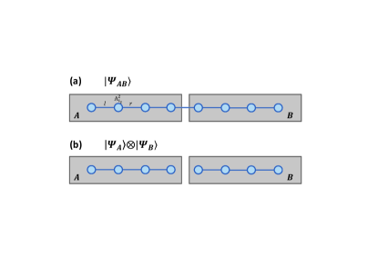
Figure 1: (Color online) $A$ and $B$ are two independent 1D Heisenberg spin chains, each containing $L$-sites. (a) A schematic MPS representation of the $A\oplus B$ super-system. (b) Schematic MPS representations of the sub-systems $A$ and $B$. Each filled circle represents a tensor $A^{i}_{i_{k}}$ and the line connecting them represents their virtual bonds $l$ and $r$.

Alternatively, we can calculate the ground state energies $E_{A}$ and $E_{B}$ of the sub-systems $A$ and $B$ separately [see Fig. 1(b)] and add them to get the total energy of the 2$L$ spin chain. We calculate the SCE for 2$L$ up to 128 sites, using the Schmidt cut-off $D$=1 - 24. We observe that the SCE $\Delta E$=0 for all the spin chain lengths and the Schmidt cut-off $D$, demonstrating that MPS is indeed size-consistent in 1D. Because it has been demonstrated that the DMRG method is equivalent to the variational MPS method, the DMRG method is also size-consistent in 1D. This implies that the MPS/DMRG method can maintain the accuracy of the calculations for larger systems without (at least significantly) increasing $D$, explaining its success in 1D. This result is in contrast with the numerical renormalization group method Wilson (1975), in which one continuously truncates the global variational spaces, and therefore, the variational spaces of the super-system and sub-systems are different, leading to the size inconsistency and failure of the method.

We now move to the 2D case. We study the 2$L\times$2$L$ Heisenberg spin lattice presented in Fig. 2, which contains two non-interacting $L\times 2L$ lattices denoted by $A$ and $B$, as the exchange interactions $J$ are set to zero between the two systems as performed for the 1D spin chain. We compare two kinds of tensor networks: one is a direct generation of MPS, and the other is PEPS.

We first calculate the ground state energies of the 2$L$$\times$2$L$ lattice and $L$$\times$2$L$ lattice and their SCEs using the variational MPS method. When calculating the ground state of the $A\oplus B$ super-system, the MPS is arranged in a snaky manner as illustrated in Fig. 2(a), whereas when we calculate the ground states of $A$ and $B$ separately, the MPS is arranged in the manner illustrated in Fig. 2(b). The relative SCE, $\Delta E/E_{A\oplus B}$, for 2$L$=4, 6, 8 and Schmidt cut-off $D$=1 - 24 are shown in Fig. 3. For all the lattice sizes, the SCE $\Delta E$=0 at $D$=1. This result occurs because at $D$=1, the MPS is a direct product state, resembling the Hartree-Fock method, which is size-consistent. However, for $D>$2, the SCE first increases with $D$ up to a certain value $D_{c}$, and then decreases as $D$ increases. As shown in Fig. 3, $D_{c}$ increases with the system size, and more importantly, the SCE decays much slower as the system size increases. For the 4$\times$4 system, the SCE becomes small for $D>$16, whereas for the 6$\times$6 and 8$\times$8 system, the SCEs are still significant even for $D$=24. These results suggest that to maintain the accuracy of the method, $D$ must increase rapidly with the system size. Indeed, it has been observed that to achieve certain accuracy, the Schmidt cut-off $D$ must grow exponentially with the dimension of the lattice Liang and Pang (1994), leading to the failure of the MPS/DMRG methods at in 2D.

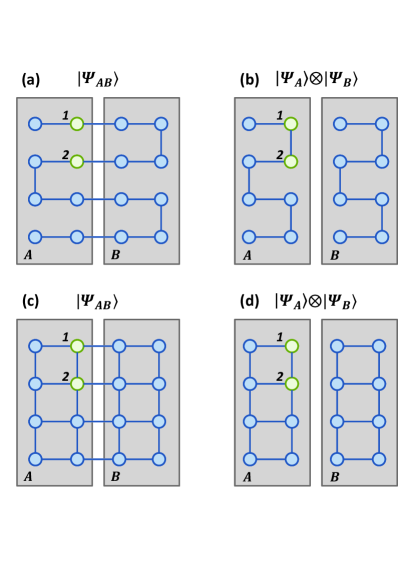
Figure 2: (Color online) $A$ and $B$ are two independent 2D Heisenberg spin lattice, each containing $L\times 2L$-sites. (a) A schematic MPS representation of the $A\oplus B$ super-system. (b) Schematic MPS representations of the sub-systems $A$ and $B$. (c) A schematic PEPS representation of the $A\oplus B$ super-system. (d) Schematic PEPS representations of the sub-systems $A$ and $B$.

PEPS is a natural generalization of MPS to two and higher dimensions from entanglement insight, whose entanglement is bonded by the number of entangled pairs and is determined by some projectors (denoted by some tensors) Verstraete and Cirac (2004a). A PEPS variational wavefunction for the $2L\times 2L$ system can be written as

$$|\Psi_{\text{PEPS}}\rangle=\sum^{d}_{i_{1,1},\ldots,i_{2\text{L},2\text{L}}=1}C\left(\left\{A^{i_{m,n}}(m,n)\right\}\right)|i_{1,1},\ldots,i_{2\text{L},2\text{L}}\rangle.$$ (2)

Similar to MPS, $d$ is the dimension of the physical indices ${i_{m,n}}$. The tensors $\{A^{i_{m,n}}(m,n)\}$ are now four index tensors $A_{u,d,l,r}$ that connects to their neighbor tensors in the up, down, left and right directions with bond dimension $D$, except for the tensors at the four borders of the lattice. The function $C$ contracts all the virtual indices $u$,$d$,$l$,$r$ of all the tensors. $D$ is the dimension of the virtual states. We obtain the ground state using a variational method following Refs. Isacsson and Syljuåsen (2006).

PEPS has been demonstrated to be successful in treating 2D many-body systems Verstraete and Cirac (2004a); Murg et al. (2007); Isacsson and Syljuåsen (2006); Fernández-González et al. (2012); Ji et al. (2011); Corboz et al. (2011). For the Heisenberg model studied here, the PEPS method converges very well to the exact ground state even with a small Schmidt cut-off $D$=4, for the 4$\times$4 lattice. The relative SCEs, $\Delta E/E_{A\oplus B}$, of the PEPS are also presented in Fig. 3 and compared with those of the MPS method for 2$L$=4, 6, 8. Unlike the MPS, we observe that the SCEs of PEPS are all zero within numerical error, regardless of the size and Schmidt cut-off $D$, confirming that PEPS is indeed size-consistent. This implies that we can use a relatively small Schmidt cut-off even for a large system without losing accuracy.

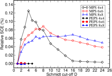
Figure 3: (Color online) The relative SCEs of the 2D Heisenberg model as functions of the Schmidt cut-off for different lattice sizes. The relative SCEs of MPS are represented by in open labels, whereas the relative SCEs of PEPS are represented by solid labels.

With the former intuitive results, we can now discuss the general size consistency of the TNS. To be a size-consistent tensor network theory, the direct product of any wave functions $|\Psi_{A}\rangle$ and $|\Psi_{B}\rangle$ (for two non-interacting sub-systems $A$ and $B$,respectively), which are represented in the tensor network of some fixed bond dimension $D$, should be presented exactly by a tensor network of the super-system $\Psi_{A\oplus B}$ with the same $D$. For the MPS case, this can be done in 1D systems but not in 2D systems. More explicitly, the states of the sub-systems $A$ and $B$, $|\Psi_{A}\rangle$ and $|\Psi_{B}\rangle$, can be represented in the form of Eq.(1) with tensors $A^{i_{1}}(1),\cdots,A^{i_{L}}(L)$ and $B^{i_{1}}(1),\cdots,B^{i_{L}}(L)$, respectively. Note that the direct product of the two sub-systems can be represented in MPS form with $D$=1. Therefore, we can construct a MPS for the supersystem in the form of Eq.(1) with tensors $C^{i_{1}}(1),\cdots,C^{i_{2L}}(2L)$ (with bond dimension $D$), which are defined as:

$$C^{i_{k}}(k) = A^{i_{k}}(k),\,\text{when}\,k=1,2,\cdots,L-1$$ (3)

$$C^{i_{L}}_{l,1}(L) = A^{i_{L}}(L),\,\text{else}\,C^{i_{L}}(L)==0$$

$$C^{i_{L+1}}_{1,m}(L+1) = B^{i_{L}}(L),\,\text{else}\,C^{i_{L+1}}(L+1)==0$$

$$C^{i_{L+k}}(L+k) = B^{i_{L}}(k),\,\text{when}\,k=1,2,\cdots,L-1$$

This MPS is in the super-system $\Psi_{A\oplus B}$ with the same dimension $D$ and exactly equal to the direct product of $|\Psi_{A}\rangle$ and $|\Psi_{B}\rangle$.

A similar construction can be used in two dimensions; however, the resulting state is not in the MPS space in Fig. 2 (a) and (b), because there are some additional bonds in the new state beyond MPS, such as the bond between sites 1 and 2. Therefore, there are two MPS states in the subsystem, whose direct product is not in the MPS space of the super-system, and the MPS method is not size-consistent. The physical reason why MPS is not size-consistent in 2D is described as follows. The entanglement between sites 1 and 2 in sub-system A has to go through B, i.e., the entanglement in a system un-physically depends on the states of another system that has no interaction with the system at all. In this case, if $\Psi_{A\oplus B}$ is written as the direct product of $\Psi_{A}$ and $\Psi_{B}$, similar to Eq. 3, there would be no entanglement between sites 1 and 2 at all.

Fortunately, this result would not occur for the PEPS in 2D. By performing the same trick as in the 1D MPS for all edges linking the two sub-systems in Fig. 2(c) and using the same tensors at all other sites as those of the sub-systems. The resulting state is exactly equal to the product state of the subsystems and in the PEPS space with the same bond dimension $D$.

From the discussion above, we find that the size consistency of a tensor network method can be reduced to the geometry structure of the network and is independent of the system Hamiltonian. The network should have the same structure when two sub-lattices merge into a super-lattice or a super-lattice separates into two sub-lattices, i.e., no additional tensor bonds beyond those in the super-lattice should be presented in the sub-lattice networks. This simple criterion can readily exclude many of the tensor networks. We also note that whereas the truncated CI method suffers from its lack of size consistency, the great advantage of tensor network methods is that much easier to construct a size-consistent theory based on TNS.

The entanglement rule and the size consistency rule originates from the different points of view. In fact, the entanglement is concerned with the global property of the state, whereas the size consistency criterion, defined by the energy relation, is simply determined by the local reduced density matrices. The relation between the global state and its local reduced density matrices is very complicated and subtleColeman (1963). A theory satisfying the size consistency condition may have no entanglement, e.g., the Hartree-Fock and Gutzwiller methods Gutzwiller (1963), whose variational spaces are product states.

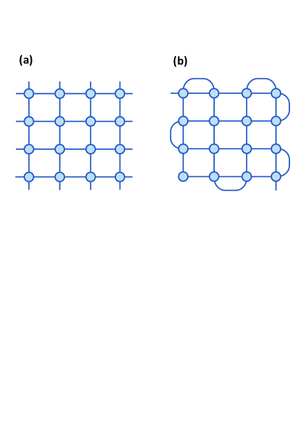
Figure 4: (Color online) The two types of string bond states (SBSs) proposed in Ref.Schuch et al. (2008): (a) horizontal and vertical lines, and (b) a long line covers all the sites.

On the other hand, a theory whose states in the variational space satisfy the area law is not necessarily size-consistent. Figure 4 depicts two types of string bond states (SBSs) proposed by Schuch et al. Schuch et al. (2008), which both satisfy the area law. Whereas the lines SBS in Fig. 4(a) is size-consistent, the long line SBS in Fig. 4 (b) is not. This can be seen by dividing the lattice in Fig. 4(b) into two parts, the long line SBS of the sub-systems have additional bonds beyond those in the super-system.

We note that size consistency is only a necessary but not a sufficient requirement for a “good” theory. Size consistency describes only the additivity property of the energy. If we are only interested in the energies, even a low level a size-consistent theory, such as the Hartree-Fock method or Gutzwiller method etc., may provide a very good approximation to separate the quantum phases from energy. However, in many cases, we are often interested in more subtle physical properties such as the correlations of the ground states, for which these theories may fail. Therefore, a good tensor network method for quantum many-body problems should satisfy the following constraints: (i) The theory must be size-consistent; (ii) The theory must satisfy proper entanglement scaling with system sizes; (iii) The theory must be systematically improvable via some controlling parameters and eventually converge to the exact results; and finally (iv) The theory must be efficient, such that the computational cost scaling with the controlling parameters is modest.

To summarize, we have discussed the size consistency of tensor network methods for quantum many-body systems. We demonstrate that the size consistency is essential for the success of the tensor network method for the quantum many-body problem, which is responsible for the failure of MPS and the success of PEPS in 2D. We further demonstrate that a tensor network state satisfying the area law is not necessarily size-consistent. Size consistency therefore provides an independent and tight constraint in constructing the tensor network method. We propose four criteria for a good tensor network method for the quantum many-body problem.

LH acknowledges the support from the Chinese National Fundamental Research Program 2011CB921200, and the National Natural Science Funds for Distinguished Young Scholars. YH acknowledges the support from the Central Universities WK2470000004, WK2470000006, WJ2470000007 and NSFC11105135.

References

- Anderson (1972) P. W. Anderson, Science 177, 393 (1972).
- Sachdev (2011) S. Sachdev, Quantum Phase Transitions (Cambridge University Press, 2011).
- Verstraete et al. (2008) F. Verstraete, V. Murg, and J. Cirac, Advances in Physics 57, 143 (2008).
- Östlund and Rommer (1995) S. Östlund and S. Rommer, Phys. Rev. Lett. 75, 3537 (1995).
- Kl¨¹mper et al. (1993) A. Kl¨¹mper, A. Schadschneider, and J. Zittartz, EPL 24, 293 (1993).
- Fannes et al. (1992) M. Fannes, B. Nachtergaele, and R. Werner, Communications in Mathematical Physics 144, 443 (1992).
- Verstraete and Cirac (2004a) F. Verstraete and J. I. Cirac, cond-mat/0407066 (2004a).
- Verstraete and Cirac (2004b) F. Verstraete and J. I. Cirac, Phys. Rev. A 70, 060302 (2004b).
- Amico et al. (2008) L. Amico, R. Fazio, A. Osterloh, and V. Vedral, Rev. Mod. Phys. 80, 517 (2008).
- White (1992) S. R. White, Phys. Rev. Lett. 69, 2863 (1992).
- White (1993) S. R. White, Phys. Rev. B 48, 10345 (1993).
- Wolf (2006) M. M. Wolf, Phys. Rev. Lett. 96, 010404 (2006).
- Kraus et al. (2010) C. V. Kraus, N. Schuch, F. Verstraete, and J. I. Cirac, Phys. Rev. A 81, 052338 (2010).
- Verstraete et al. (2006) F. Verstraete, M. M. Wolf, D. Perez-Garcia, and J. I. Cirac, Phys. Rev. Lett. 96, 220601 (2006).
- Löwdin (1956) P. O. Löwdin, Adv. Phys. 5, 1 (1956).
- Pople et al. (1987) J. A. Pople, M. Head-Gordon, and K. Raghavachari, The Journal of Chemical Physics 87, 5968 (1987).
- Szabo and Ostlund (1989) A. Szabo and N. S. Ostlund, Modern Quantum Chemistry (Dover Publications, 1989).
- Wilson (1975) K. G. Wilson, Rev. Mod. Phys. 47, 773 (1975).
- Liang and Pang (1994) S. Liang and H. Pang, Phys. Rev. B 49, 9214 (1994).
- Isacsson and Syljuåsen (2006) A. Isacsson and O. F. Syljuåsen, Phys. Rev. E 74, 026701 (2006).
- Murg et al. (2007) V. Murg, F. Verstraete, and J. I. Cirac, Phys. Rev. A 75, 033605 (2007).
- Fernández-González et al. (2012) C. Fernández-González, N. Schuch, M. M. Wolf, J. I. Cirac, and D. Pérez-García, Phys. Rev. Lett. 109, 260401 (2012).
- Ji et al. (2011) S. Ji, C. Ates, and I. Lesanovsky, Phys. Rev. Lett. 107, 060406 (2011).
- Corboz et al. (2011) P. Corboz, A. M. Läuchli, K. Penc, M. Troyer, and F. Mila, Phys. Rev. Lett. 107, 215301 (2011).
- Coleman (1963) A. J. Coleman, Rev. Mod. Phys. 35, 668 (1963).
- Gutzwiller (1963) M. C. Gutzwiller, Phys. Rev. Lett. 10, 159 (1963).
- Schuch et al. (2008) N. Schuch, M. M. Wolf, F. Verstraete, and J. I. Cirac, Phys. Rev. Lett. 100, 040501 (2008).