Multi-scale dynamical analysis (MSDA) of sea level records versus PDO, AMO, and NAO indexes

Abstract

Herein I propose a multi-scale dynamical analysis to facilitate the physical interpretation of tide gauge records. The technique uses graphical diagrams. It is applied to six secular-long tide gauge records representative of the world oceans: Sydney, Pacific coast of Australia; Fremantle, Indian Ocean coast of Australia; New York City, Atlantic coast of USA; Honolulu, U.S. state of Hawaii; San Diego, U.S. state of California; and Venice, Mediterranean Sea, Italy. For comparison, an equivalent analysis is applied to the Pacific Decadal Oscillation (PDO) index and to the Atlantic Multidecadal Oscillation (AMO) index. Finally, a global reconstruction of sea level (Jevrejeva et al., 2008) and a reconstruction of the North Atlantic Oscillation (NAO) index (Luterbacher et al., 2002) are analyzed and compared: both sequences cover about three centuries from 1700 to 2000. The proposed methodology quickly highlights oscillations and teleconnections among the records at the decadal and multidecadal scales. At the secular time scales tide gauge records present relatively small (positive or negative) accelerations, as found in other studies (Houston and Dean, 2011). On the contrary, from the decadal to the secular scales (up to 110-year intervals) the tide gauge accelerations oscillate significantly from positive to negative values mostly following the PDO, AMO and NAO oscillations. In particular, the influence of a large quasi 60-70 year natural oscillation is clearly demonstrated in these records. The multiscale dynamical evolutions of the rate and of the amplitude of the annual seasonal cycle of the chosen six tide gauge records are also studied.

$\sim$

Cite this article as: Scafetta, N., 2013. Multi-scale dynamical analysis (MSDA) of sea level records vs. PDO, AMO, and NAO indexes. Climate Dynamics. DOI: 10.1007/s00382-013-1771-3

1 Introduction

Understanding the complex dynamics of sea level and tide gauge records is necessary for testing models of sea level changes against data and to provide local governments with efficient forecasts for planning appropriate actions to protect communities from possible sea inundation and for other civil purposes. Long-term sea level variations are driven by numerous coupled processes arising from an interaction of eustatic sea level rise and glacial isostatic subsidence, long-term tidal and solar cycles, oscillations of ocean circulation, variations in temperature and/or salinity and other factors that can be also characteristic of the specific geographical location (e.g: Douglas, 1992; Dean and Houston, 2013; Houston and Dean, 2011; Levermann et al., 2005; Mörner, 1989, 1990, 2010; Sallenger et al., 2012; Woodworth, 1990).

Despite their intrinsic dynamical complexity, tide gauge records are often analyzed using simplistic mathematical approaches, such as fitting one given time interval with a second order polynomial of the type:

$$f(t)=\frac{1}{2}a(t-t_{0})^{2}+v_{0}(t-t_{0})+c_{0},$$ (1)

where $a$ is the sea level average acceleration during the fitted period (it does not depend on $t_{0}$), $v_{0}$ is the sea level rate at $t_{0}$, and $c_{0}$ is the average level at $t_{0}$. The reference date, $t_{0}$, can be changed as necessary.

However, it is easy to demonstrate that fitting tide gauge records within just one generic period can yield severely ambiguous results. In fact, complex signals are characterized by specific multi-scale patterns that a regression analysis on a fixed time interval can obscure. Simply changing the length and the time period used for the analysis can significantly alter the values of the regression parameters.

For example, sea-level accelerations are critical components for understanding the forces that determine their dynamical evolution and for projecting future sea levels. Without any acceleration, the 20th century global sea-level average trend of $\sim 1.7$ $mm/year$ would produce a rise of only $\sim 153$ $mm$ from 2010 to 2100 (Houston and Dean, 2011). However, the scientific literature reports apparently contrasting results about the acceleration values. Let us discuss a few cases.

(1) Church and White (2006) used secular-long time series and estimated that the global sea level from 1880 to 2004 experienced a modest acceleration, $a=0.013\pm 0.006$ $mm/year^{2}$. Church and White (2011) repeated the analysis for the period 1880-2009 and found a slightly smaller value, $a=0.009\pm 0.004$ $mm/year^{2}$. Houston and Dean (2011) analyzed 25 tide gauges for the period 1930 to 2010 and found a mean negative acceleration, $a=-0.0123\pm 0.0104$ $mm/year^{2}$ (95%), where the 17 gauge records for the Atlantic zone had an average acceleration of $a=-0.0138\pm 0.0148$ $mm/year^{2}$ (95%) and 8 gauge records from the Pacific coast had an average acceleration of $a=-0.0091\pm 0.0096$ $mm/year^{2}$(95%). If the above (positive or negative) acceleration values persist also for the 21st century, their overall effect would be modest: the average sea level could rise $\sim 150\pm 100$ $mm$ from 2010 to 2100 by taking into account also the $\sim 1.7$ $mm/year$ average linear rate.

(2) Sallenger et al. (2012) analyzed the period 1950-2009 and found that numerous locations of the Atlantic coast of North America are characterized by strong positive accelerations. Similar results were found also by Boon (2012), who used quadratic polynomial regressions to analyze a number of U.S. and Canadian tide gauge records over the 43 years period from 1969 to 2011. For example, in New York City the acceleration during the 1950-2009 period was estimated to be $a=0.044\pm 0.030$ $mm/year^{2}$ ($1\sigma$ error, annual resolution) (Sallenger et al., 2012, supplementary figure S7). For the periods 1960-2009 and 1970-2009 the acceleration values would progressively increase: $a=0.083\pm 0.049$ $mm/year^{2}$ and $a=0.133\pm 0.093$ $mm/year^{2}$, respectively. The progressive increase of the acceleration value was claimed to depart from past values and was interpreted as due to the anthropogenic warming of the last decades causing significant changes in the strength of the Atlantic Meridional overturning circulation and of the Gulf Stream. Evidently, high positive acceleration values and their progressive increase would be quite alarming if this trend persists also during the 21st century, as the anthropogenic global warming theory would predict (IPCC, 2007). For example, in New York City, if the 1970-2009 acceleration remains constant during the 21st century and the 1970-2009 quadratic polynomial fit is used to extrapolate the 21st century sea level rise, the sea level could increase by $\sim 1129\pm 480$ $mm$ from 2000 to 2100. For New York City, Boon (2012) used his 1969-2011 quadratic polynomial fit to project a sea level rise of 390-750 mm above the 1983-2001 sea level mean by 2050. However, I observe that using the 1900-2000 quadratic polynomial fit extrapolation, which produces an acceleration of just $a=0.0032\pm 0.0079$ $mm/year^{2}$, in New York City the sea level could increase by just $\sim 332\pm 60$ $mm$ from 2000 to 2100 (that is mostly due to the linear rate of $v_{0}=3.16\pm 0.41$ mm/year), which makes a significant difference.

(3) Dean and Houston (2013) analyzed 456 globally distributed monthly tide gauge records and satellite measured records for the period 1993-2011 and found negative average accelerations (with a relatively large uncertainty), $a=-0.041$ $mm/year^{2}$ (gauges) vs. $a=-0.083$ $mm/year^{2}$ (satellites). Therefore, during the last two decades the sea level accelerations have been mostly negative at numerous locations. If these negative accelerations persist during the 21st century, sea level rates would significantly slow down and, eventually, sea levels could even decrease in numerous locations.

(4) Boretti (2012) analyzed two century-long tide gauge records referring to the east and west coast of Australia, Sydney and Fremantle, and found secular accelerations of $a=0.014$ $mm/year^{2}$ and $a=-0.0023$ $mm/year^{2}$, respectively, and for the 20-year period from Jan/1990 to Dec/2009 he found accelerations of $a=0.37$ $mm/year^{2}$ and $a=-0.6$8 $mm/year^{2}$, respectively. Hunter and Brown (2013) used the same tide gauge records used by Boretti but with an annual resolution, and for the 21-year period from 1990 to 2010 found $a=0.44\pm 0.34$ $mm/year^{2}$ (Sydney) and $a=-0.60\pm 0.70$ $mm/year^{2}$ (Fremantle); they also reported the global accelerations measured by satellite altimeters for the 1993-2009 period, $a=-0.027\pm 0.114$ $mm/year^{2}$, and from theoretical computer climate models for the period 1990-2009, $a=0.078\pm 0.107$ $mm/year^{2}$.

As it is evident by comparing the above apparently contrasting results, the evaluated accelerations appear to strongly depend not only on the location, but also on the time intervals chosen for the regression analysis. Sea level records are not just randomly evolving around an acceleration background trending, but they appear to be characterized by complex natural oscillations. Consequently, each of the above estimated acceleration values, by alone, may not tell us much about the true long-range dynamics of tide gauge records. Indeed, those numbers may be highly ambiguous and may generate confusion to some readers, e.g. policy makers, who may wonder whether sea levels are strongly accelerating, or strongly decelerating, or not accelerating or decelerating at all. Moreover, comparing sea level acceleration values from different locations measured using records of different lengths and periods (e.g. as done in: Houston and Dean, 2011; Woodworth et al., 2009) may be equally misleading in presence of oscillations.

Indeed, quasi 20-year and 60-year oscillations have been found in sea level records (Chambers et al., 2012; Jevrejeva et al., 2008; Mörner, 2010), although the patterns referring to individual tide gauge records appear to be quite complex and inhomogeneous (e.g. Woodworth et al., 2009). Cyclic changes could partially explain why the accelerations of these records are close to zero when quasi secular-long records are analyzed (Church and White, 2011; Houston and Dean, 2011), while the same records may present large positive accelerations when short periods of 40-60 years between 1950 to 2009 are analyzed, as done by Sallenger et al. (2012) and by Boon (2012). Cyclic changes could also explain the large volatility measured in the acceleration values at the decadal and bi-decadal scales. Indeed, quasi decadal, bi-decadal and 50-90 year oscillations have been found for centuries and millennia in numerous climate and marine records (Chylek et al., 2011; Klyashtorin et al., 2009; Knudsen et al., 2011; Kobashi et al., 2010; Mazzarella and Scafetta, 2012; Mörner, 1989, 1990). Since 1850 quasi decadal, bidecadal and 60-year oscillations have been found in global temperature records, are typical astronomical/solar oscillations and will likely exist also in the future (Ogurtsov et al., 2002; Scafetta, 2010, 2012a, 2012b; Scafetta and Willson, 2013; Soon and Legates, 2013). Thus, it is legitimate to expect that equivalent oscillations (with appropriate phase shifts depending on the geographical location) may characterize numerous tide gauge records too.

For example, it is possible that Sallenger et al. (2012) found very large positive acceleration values in the tide gauge records for New York City and other U.S. Atlantic cities (the so-called “hot-spots”) simply because these authors compared trends between the periods 1950-1979 and 1980-2009 that could follow from a valley to a peak the 60-year oscillation commonly found in the Atlantic Multidecadal Oscillation (AMO), in the Pacific Decadal Oscillation (PDO) and in the North Atlantic Oscillation (NAO) indexes (Knudsen et al., 2011; Loehle and Scafetta, 2011; Mazzarella and Scafetta, 2012). This 60-year oscillation may have made the tide gauge record for New York City as well as for other U.S. Atlantic cities concave from 1950 to 2009. A similar critique would apply also to the results by Boon (2012), who used 1969-2011 quadratic polynomial fits to project future sea level trends up to 2050. For the same reason, Dean and Houston (2013) found significant negative accelerations for the period 1993-2011 likely because the bidecadal and the 60-year oscillations may have been bending down during this period by making the tide gauge records momentarily convex. Below, I will demonstrate the validity of the critique.

Herein I propose a multi-scale dynamical analysis (MSDA) methodology to study dynamical patterns revealed in tide gauge records. MSDA uses colored palette diagrams to represent local accelerations, rates and average annual seasonal amplitudes at multiple scales and time periods. This methodology aims: (1) to provide a comprehensive dynamical picture of climatic records; (2) to facilitate their physical interpretation by highlighting interconnections and dynamical couplings among climatic indexes; (3) to avoid possible embarrassing ambiguities emerging from arbitrary choices of the time intervals used for the regression analysis; (4) to develop more appropriate forecast models that take into account the real dynamics of these records.

The MSDA visualization technique is used to analyze dynamical details in six secular-long tide gauge records that approximately provide a global coverage of the world oceans. Sydney, Fremantle, and New York City were also analyzed using more simplistic methodologies in Boretti (2012), Hunter and Brown (2013) and Sallenger et al. (2012): so a reader may better appreciate the high performance of MSDA by comparing its results with those recently published by other scientists. The MSDA diagrams are compared versus equivalent diagrams referring to the PDO index and to the AMO index to provide a physical interpretation of the results. The tide gauge records of Honolulu, San Diego and Venice are briefly studied to provide a more worldwide picture of the situation and to highlight additional teleconnection patterns among different regions. Finally, MSDA diagrams are used to compare a global reconstruction of sea level (Jevrejeva et al., 2008) and a reconstruction of the NAO index (Luterbacher et al., 1999): both sequences cover about three centuries since 1700 and can be used to highlight a possible physical coupling and to confirm the presence of a major 60-70 year natural oscillation in these records.

period	Sydney	Fremantle	New York
1/1886 - 12-2010	$+0.014\pm 0.003$
1/1897 - 12/2010	$+0.016\pm 0.003$	$-0.007\pm 0.006$	$+0.008\pm 0.005$
6/1914 - 12/2010	$+0.006\pm 0.005$	$-0.018\pm 0.009$	$+0.002\pm 0.007$
1/1914 - 12/1993	$+0.022\pm 0.008$	$-0.080\pm 0.014$	$-0.026\pm 0.011$
1/1950 - 12/2009	$+0.014\pm 0.016$	$+0.083\pm 0.029$	$+0.043\pm 0.023$
1/1989 - 12/2010	$+0.436\pm 0.201$	$-0.054\pm 0.360$	$-0.158\pm 0.292$
1/1990 - 12/2009	$+0.372\pm 0.257$	$-0.678\pm 0.458$	$-0.337\pm 0.372$
1/1990 - 12/2010	$+0.361\pm 0.228$	$-0.598\pm 0.400$	$+0.061\pm 0.328$
1/1991 - 12/2010	$+0.039\pm 0.254$	$-0.739\pm 0.459$	$+0.423\pm 0.372$
1/1992 - 12/2010	$-0.233\pm 0.287$	$-0.920\pm 0.520$	$+0.676\pm 0.435$
1/1993 - 12/2010	$-0.549\pm 0.327$	$-0.920\pm 0.600$	$+0.923\pm 0.497$

Table 1: Tide gauge level accelerations ($mm/year^{2}$) in Sydney, Fremantle and New York within arbitrary time intervals using Eq. 1.

period	Eq. 1 - year	Eq. 1 - month	Eq. 2 - month
1/1893 - 12/2010	$0.0102\pm 0.0052$	$+0.0078\pm 0.0042$	$+0.0073\pm 0.0031$
1/1900 - 12/2010	$0.0075\pm 0.0062$	$+0.0046\pm 0.0049$	$+0.0041\pm 0.0037$
1/1910 - 12/2010	$0.0028\pm 0.0078$	$-0.0008\pm 0.0061$	$-0.0014\pm 0.0046$
1/1920 - 12/2010	$0.0005\pm 0.0102$	$-0.0042\pm 0.0079$	$-0.0048\pm 0.0060$
1/1930 - 12/2010	$0.0053\pm 0.0138$	$-0.0013\pm 0.0106$	$-0.0020\pm 0.0081$
1/1940 - 12/2010	$0.0414\pm 0.0188$	$+0.0334\pm 0.0148$	$+0.0328\pm 0.0114$
1/1950 - 12/2010	$0.0687\pm 0.0286$	$+0.0583\pm 0.0216$	$+0.0583\pm 0.0169$
1/1960 - 12/2010	$0.1203\pm 0.0455$	$+0.1069\pm 0.0341$	$+0.1086\pm 0.0265$
1/1970 - 12/2010	$0.1941\pm 0.0830$	$+0.1725\pm 0.0601$	$+0.1797\pm 0.0469$
1/1980 - 12/2010	$0.0644\pm 0.1762$	$+0.0163\pm 0.1222$	$+0.0413\pm 0.0950$
1/1990 - 12/2010	$0.2223\pm 0.4678$	$+0.0606\pm 0.3284$	$+0.1096\pm 0.2553$
1/2000 - 12/2010	$2.2596\pm 1.643$	$+2.5584\pm 1.761$	$+2.1697\pm 1.249$

Table 2: Analysis of the acceleration error-bars for the tide gauge record of New York City within different intervals and using: (1) Eq. 1 and the annual average record; (2) Eq. 1 and the monthly average record; (3) Eq. 2 and the monthly average record. The methodology (3) produces the smallest error-bars.

2 Data

Tide gauge records were downloaded from the Permanent Service for Mean Sea Level (PSMSL) (Woodworth and Player, 2003; PSMLS, 2013). The following six monthly resolution records are used: Sydney (Fort Denison, ID #65, Jan/1886 - Dec/1993; Fort Denison 2, ID #196, Jun/1914 - Dec/2010); Fremantle (ID #111, Jan/1897 - Dec/2010); and New York City (the Battery, ID #12, Jan/1856 - Dec/2011); Honolulu (ID #155, Jan/1905 - Dec/2011); San Diego (ID #158, Jan/1906 - Dec/2011); and Venice (ID #168, Jan/1909 - Dec/2000). The two records from Sydney are practically identical during the overlapping period and are combined to form a sequence from 1886 to 2010.

The following monthly records are also used: the Pacific Decadal Oscillation (PDO) index (Jan/1900 - Jan/2013); the Atlantic Multidecadal Oscillation (AMO) index (Jan/1856 - Jan/2013). The PDO and AMO indexes represent modes of variability occurring in the Pacific Ocean and in the North Atlantic Ocean, respectively, which have their principal expression in the sea surface temperature field once linear trends are removed. The oscillations revealed in these records likely arise from a quasi-predictable variability of the ocean–atmosphere system observed for centuries and millenia (Klyashtorin et al., 2009; Knudsen et al., 2011; Mantua et al., 1997; Scafetta, 2010, 2012b; Schlesinger and Ramankutty, 1994), which is expected to influence tide gauge records as well given their dependency on global temperature related climatic changes.

Finally, a global reconstruction of sea level (Jevrejeva et al., 2008) and a reconstruction of the North Atlantic Oscillation (NAO) (Luterbacher et al., 1999, 2002) are also studied: both sequences cover about three centuries from 1700 to 2000. The NAO index is defined as the average air pressure difference between a low latitude region (e.g. Azores) and a high latitude region (e.g. Iceland). These longer records are used to demonstrate the existence of a quasi 60-70 year natural oscillation, which needs to be taken into account for correctly interpreting the results obtained by using multidecadal-long tide gauge records.

Let us run a test to demonstrate that fitting tide gauge records within fixed periods, as done in the studies summarized in the Introduction, yields severely ambiguous results. I used Eq. 1 to fit generic intervals and the results referring to Sydney, Fremantle and New York City are reported in Table 1. The acceleration values change greatly from significantly positive to significantly negative values. In particular, at the bidecadal scales the variation of the acceleration can be quite significant and sudden. For example, for Sydney a strong positive acceleration, $a=+0.36\pm 0.23$ $mm/year^{2}$, is found for the 21-year period from Jan/1990 to Dec/2010 (as found also in Hunter and Brown, 2013), but a strong negative acceleration, $a=-0.55\pm 0.32$ $mm/year^{2}$, is found for the 18-year period from Jan/1993 to Dec/2010. The results obtained for Fremantle are also interesting: always negative acceleration values are found with the exception of the 60-year period 1950-2009 (which is the period chosen by Sallenger et al., 2012) when the acceleration is significantly positive. Thus, tide gauge records are statistically and dynamically complex, and estimating a single acceleration value within an arbitrarily chosen time interval, in particular at scales shorter than 60-70 years, can give extremely ambiguous and misleading results.

3 Multi-scale dynamical analysis (MSDA) of tide gauge records

To reduce the ambiguities highlighted above, tide gauge rates and accelerations have to be computed using moving time windows of different length. Recently Parker (2012a, b, 2013) used moving time windows of 20, 30 and 60 years to demonstrate the presence of oscillations in tide gauge records at the chosen scales. However, a comprehensive dynamical picture can be provided by analyzing all available scales at once. For example, Jevrejeva et al. (2008, figure 2) calculated acceleration coefficients using variable windows (from 10 to 290 years) of their global sea level record. This multi-scale technique and its graphical representation will be herein extended, applied to local and global sea level records and used for comparisons against the PDO, AMO and NAO indexes. The proposed methodology aims to provide sufficiently compact and eye-catching diagrams to facilitate the study of these records and to rapidly evaluate, even visually, dynamical patterns and cross-correlations among alternative climatic records that can be physically coupled and/or teleconnected to each other.

Records with a monthly resolution are adopted because the statistical error for the regression coefficients is normally smaller than using the annual resolution records due to the fact that the monthly data are not Gaussian-distributed around an average trend but are autocorrelated because constrained by the annual seasonal cycle (e.g.: Church and White, 2011, figure 3). However, the mean regression coefficients do not change significantly using the annual instead of the monthly resolution, in particular for longer scales. In any case, because the monthly tide gauge records are characterized by a strong annual seasonal cycle, Eq. 1 should be substituted with

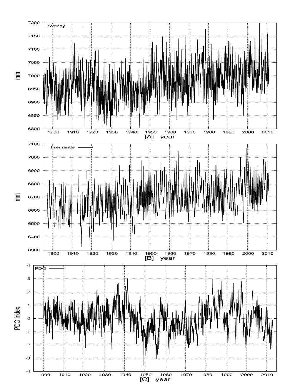
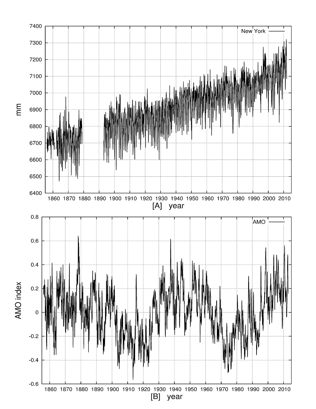
Figure 1: [A] Tide gauge record in Sydney. [B] Tide gauge record in Fremantle. [C] The Pacific Decadal Oscillation (PDO) index.

Figure 2: [A] The tide gauge record in New York. [B] The Atlantic Multidecadal Oscillation (AMO) index.

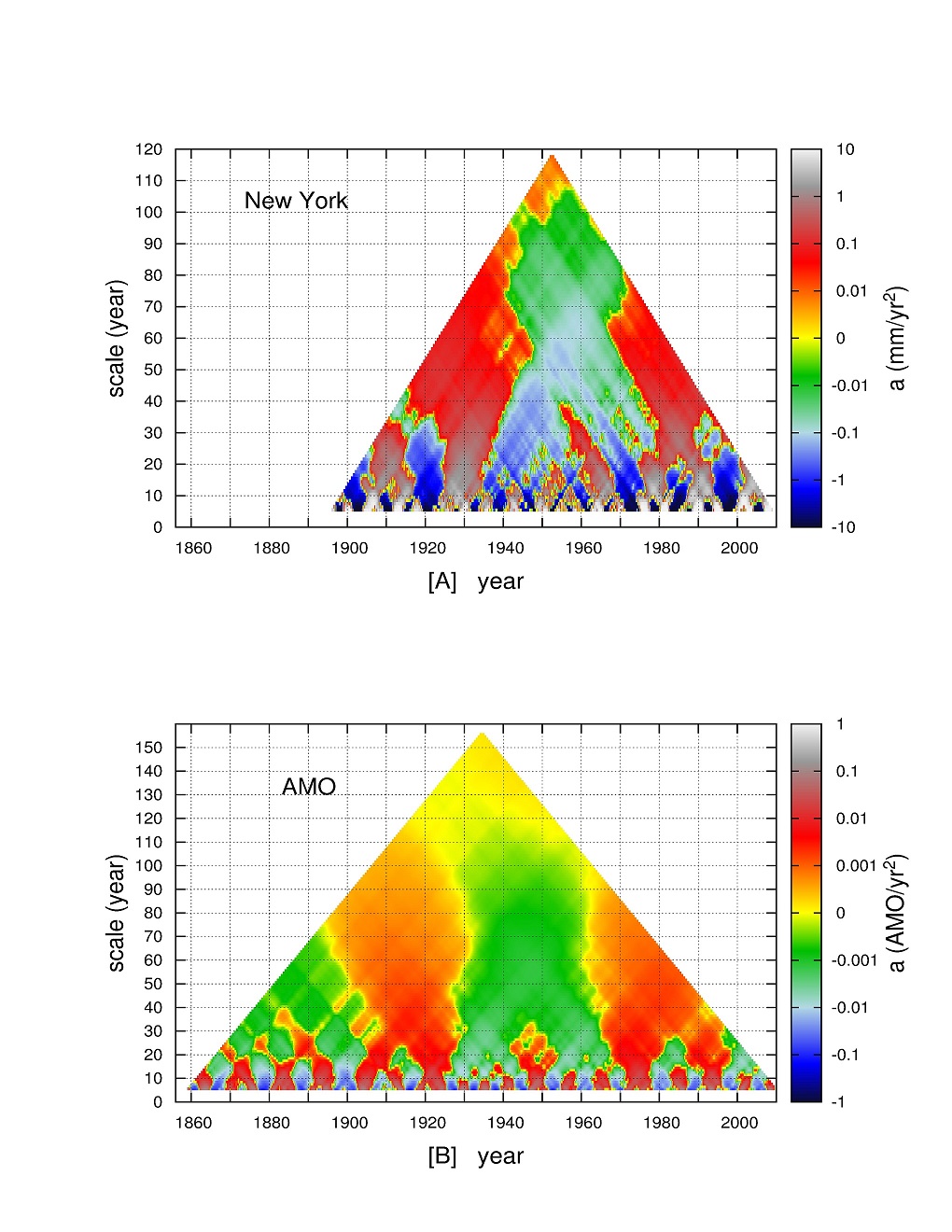
Figure 3: MSAA colored diagrams for: [A] the tide gauge record in Sydney; [B] the tide gauge record in Fremantle; [C] for the Pacific Decadal Oscillation (PDO) index (here the colors are inverted).

Figure 4: MSAA colored diagrams for: [A] the tide gauge record in New York; [B] the Atlantic Multidecadal Oscillation (AMO) index.

$$f(t)=\frac{1}{2}a(t-t_{0})^{2}+v_{0}(t-t_{0})+c_{0}+H_{c}\cos(2\pi t)+H_{s}\sin(2\pi t),$$ (2)

which takes into account the annual seasonal cycle too and could further reduce the regression uncertainties.

A test was run to evaluate how the regression error associated to the acceleration depends on different regression methodologies. Table 2 shows the difference of using: (1) the annual resolved records fit with Eq. 1 (e.g. as used in Hunter and Brown, 2013); (2) the monthly resolved records fit with Eq. 1; (3) the monthly resolved records fit with Eq. 2. The acceleration results reported in Table 2 indicate that the methodology (1) provides the worst results (= the largest error bars) at all time scales; the methodologies (2) and (3) produce almost identical average values although in the case (3) the regression algorithm would produce smaller error bars. Adopting the methodology (3) instead of the methodology (1) reduces the error bars by $\sim 40\%$. Thus, the methodology (3) should be preferred for tide gauge records if high precision is required for specific purposes.

3.1 Multi-scale acceleration analysis (MSAA)

The multi-scale acceleration analysis (MSAA) methodology evaluates the acceleration values using Eq. 2 for all possible available time window lengths, which are called “scales”, and plot the acceleration results in a colored palette diagram in function of the time position of the regression interval (abscissa) and of the scale (ordinate). The pictures are then studied for dynamical patterns and compared to equivalent diagrams referring to other records to identify possible dynamical correlations, couplings, coherences and teleconnections. No significant visible changes would be obtained by adopting Eq. 1.

Figure 1 shows the tide gauge records for Sydney and Fremantle vs. the PDO index. Figure 2 shows the tide gauge records for New York City vs. the AMO index. Figure 3 depicts the MSAA diagrams for the tide gauge records of Sydney and Fremantle, and compare them with that for the PDO index. In the latter case the colors are inverted for reasons explained below. Figure 4 depicts the MSAA diagrams for the tide gauge record of New York City (since 1893) and for the AMO index. Time scales from a minimum of 5-year periods to the total length of the data are used. The 5-year period is just a lower limit, which is chosen because it allows to detect the decadal oscillations that are known to exist in the climate system (e.g.: Scafetta, 2009, 2010, 2012a; Manzi et al., 2012).

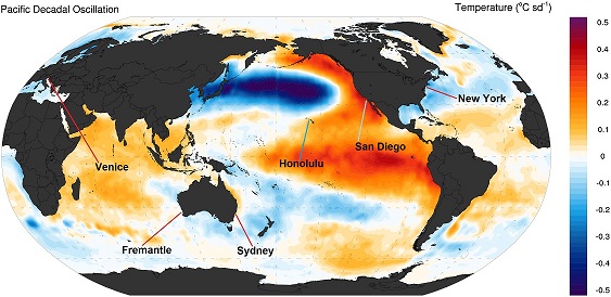
Figure 5: Pacific Decadal Oscillation (PDO), positive phase and global pattern. (Picture adapted from wikipedia, http://en.wikipedia.org/wiki/Pacific_decadal_oscillation). The figure shows also the locations of the six chosen sites studied in the paper.

The MSAA diagrams for the sea level records use a logarithmic scale for accelerations $|a|\geq 0.001$ $mm/year^{2}$ and a linear scale for $|a|\leq 0.001$ $mm/year^{2}$. The MSAA diagrams for the PDO and AMO indexes use a logarithmic scale for accelerations $|a|\geq 0.0001$ $mm/year^{2}$ and a linear scale for $|a|\leq 0.0001$ $mm/year^{2}$. Alternative scales for the acceleration, e.g. a cube root scale, can be adopted but do not give better results. The ordinate axis for the time interval scale adopts a linear scale, which produces triangle-shaped MSAA diagrams; however, a log-scale can be adopted for longer sequences and/or for highlighting the shortest scales as done in Section 4.

The interpretation of the diagrams is as follows. The color at specific coordinates, let us say at $x=1940$ and $y=40$, gives the acceleration calculated using Eq. 2 to fit the data for the 40-year long interval (scale $y=40$ years) from 1920 to 1960 (period centered in $x=1940$), and so on. Orange to red to white colors indicate incrementally positive accelerations, while green to blue to black colors indicate incrementally negative accelerations. Yellow colors indicate acceleration values very close to zero. The accelerations for the tide gauges are calculated in $mm/year^{2}$, while for the PDO and AMO indexes the units are those of these indexes, which are temperature related, per $year^{2}$.

The statistical error bars associated to the single acceleration measurements depend on the specific tide gauge record and on the scale. As Table 2 show, the error bars may vary from about $\pm 0.003$ $mm/year^{2}$ at the secular scale to about $\pm 1$ $mm/year^{2}$ at the decadal one using Eq. 2 with monthly records. However, when multiple acceleration values corresponding to a single scale are compared to determine a dynamical pattern, the average statistical error associated to it becomes smaller than the statistical error associated to each single acceleration value by a factor equal to the root of the number of degrees of freedom that may be approximately estimated to be equal to the ratio between the length of the data and the analyzed scale: e.g. for a 100-year sequence the error in the dynamical pattern may vary from about $\pm 0.003$ $mm/year^{2}$ at the secular scale to about $\pm 0.3$ $mm/year^{2}$ at the decadal one. This error bars are relatively small relatively to the maximum and minimum acceleration values observed at each scale. Therefore, the observed patterns cannot emerge from just statistical noise but are dynamically relevant. Moreover, as demonstrated below, similar patterns emerge in alternative records, which further demonstrates their physical origin.

The diagrams for the tide gauge records indicate: (1) these records are characterized by alternating periods of positive and negative accelerations at the decadal and multidecadal scales; (2) at the decadal and bi-decadal scales, strong quasi periodic oscillations are observed, as indicated by the quasi-periodic shifts from deep green regions to deep red regions; (3) at larger scales from about 30-year to 110-year, the accelerations are moderately positive both at the beginning and at the end of the records (in particular from Fremantle and New York), while in the middle of the records large regions with negative accelerations are observed, this pattern may indicate the presence of a large multidecadal oscillation that will be better discussed in Section 4; (4) the accelerations converge to small values close to zero (green-yellow-orange color) at the secular scale, which is indicated at the top of the triangle.

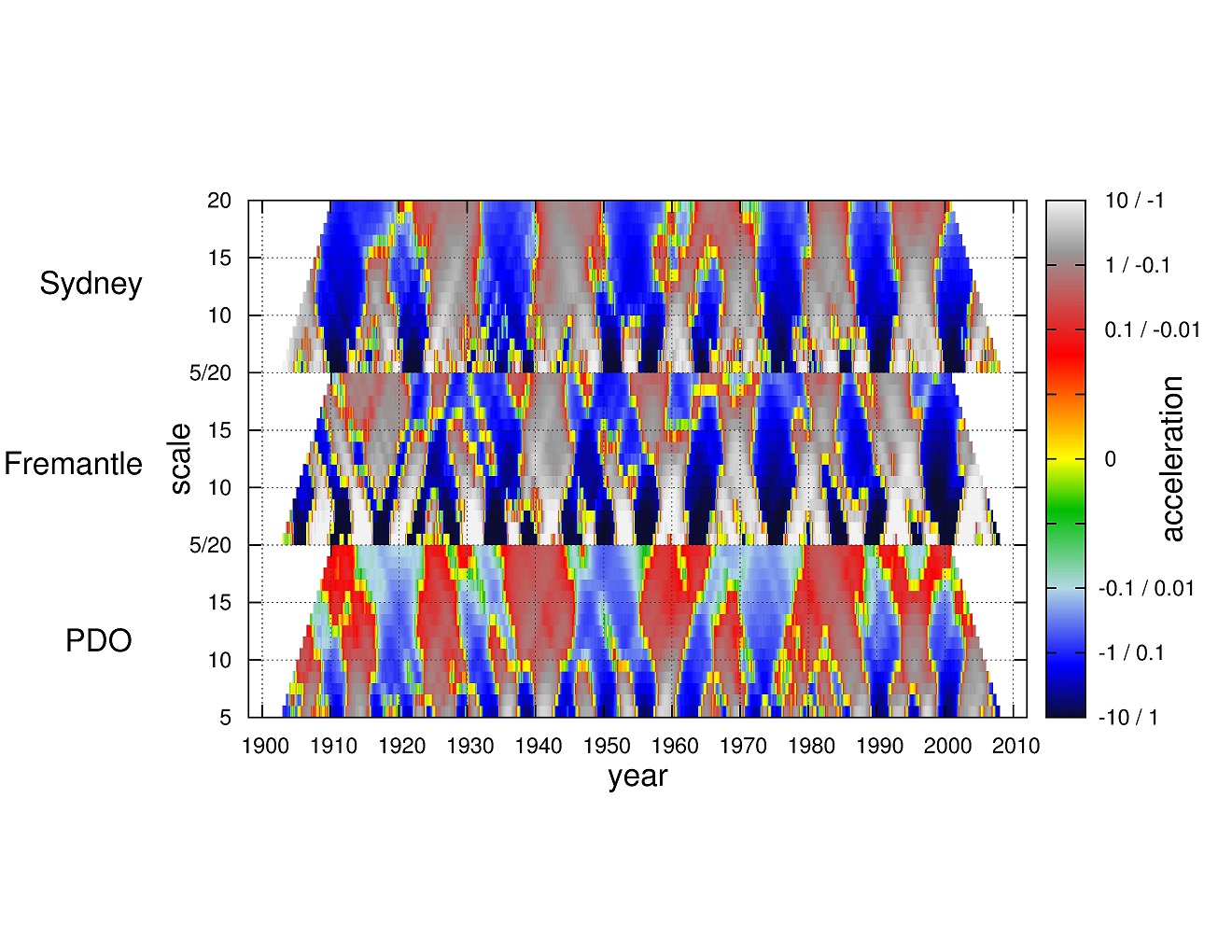
Figure 6: Zoom of Figure 3 within the scales from 5 to 20 years to highlight the good cross correlation among the three records at the decadal/bidecadal scales. Table 3 reports the cross-correlation coefficients referring to each annual scale.

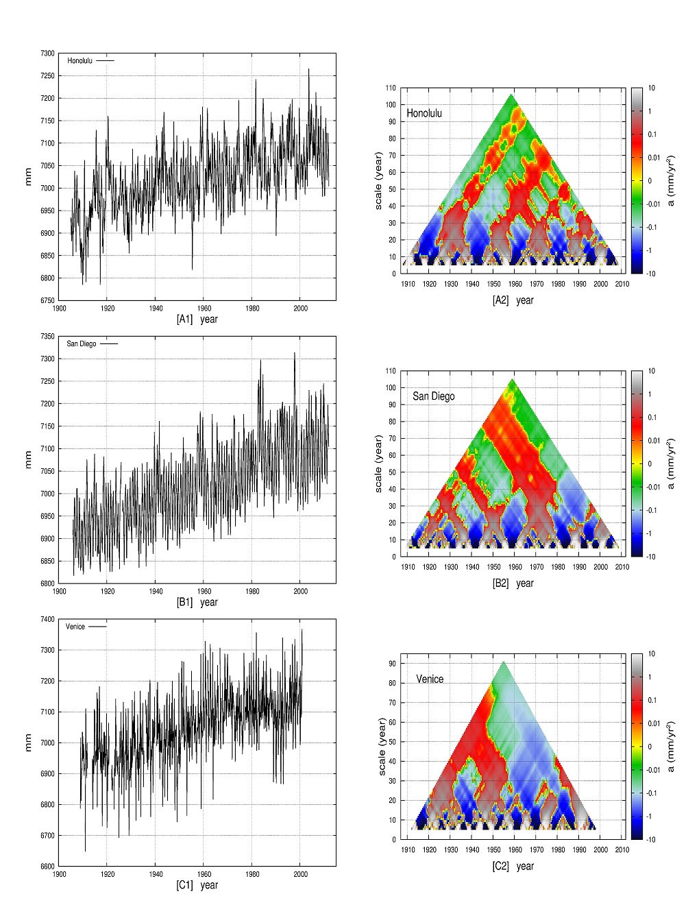
Figure 7: Tide gauge records (left) and MSAA colored diagrams (right) for: [A] Honolulu, U.S. state of Hawaii; [B] San Diego, U.S. state of California; [C] Venice, Italy.

The diagram referring to the PDO index (Fig. 3C) is plotted with inverted colors (that is, green/blue is used for positive accelerations while orange/red for negative accelerations) because when the PDO is in its “warm”, or “positive” phase, the west South Pacific (e.g. around Australia) cools while part of the eastern Pacific ocean warms; the opposite pattern occurs during the “cool” or “negative” PDO phase. For example, Figure 5 shows the PDO positive phase global pattern. So, during the PDO warm phase, the sea level around Australia may decrease, and the accelerations patterns between PDO and tide gauges in Australia may be negatively correlated.

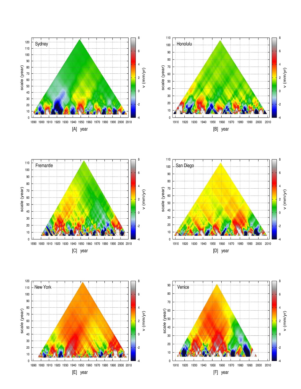
Figure 8: MSRA colored diagrams for: [A] Sydney, Australia (East coast); [B] Honolulu, U.S. state of Hawaii; [C] Fremantle, Australia (West coast); [D] San Diego, U.S. state of California; [E] New York, U.S. state of New York; [F] Venice, Italy.

The comparison between Sydney (Fig. 3A) and PDO (Fig. 3C) suggests a good negative (this is because the PDO diagram uses inverted colors) correlation, which is indicated by a same blue and red region correspondence at the 10-30 year scales. For example, note the same blue areas in both the sea level diagrams and the PDO diagram around 1910, 1920, 1930-1940, 1950-1960, 1970-1980, 1990 and 2000. At larger scales the correlation pattern is more uncertain and, as Fig. 3A shows, for Sydney the correlation with the PDO patterns becomes positive at higher scales. However, in general, long-range patterns in tide gauge records may be driven by numerous physical processes, not just the temperature related ones, but studying the precise cause of an observed pattern is beyond the purpose of the present work.

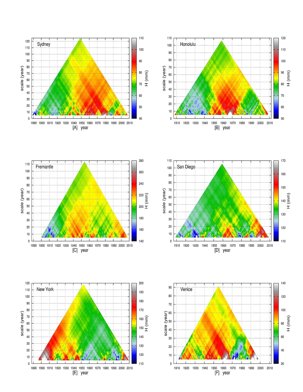
Figure 9: MSACAA colored diagrams for: [A] Sydney, Australia (East coast); [B] Honolulu, U.S. state of Hawaii; [C] Fremantle, Australia (West coast); [D] San Diego, U.S. state of California; [E] New York, U.S. state of New York; [F] Venice, Italy.

The comparison between Fremantle (Fig. 3B) and PDO (Fig. 3C) suggests extended (negative) correlations (indicated by a same color area correspondence) at almost all scales, in particular since 1930. The influence of the quasi 60-year oscillation is evident. There appears to be a small phase shift that depends on the scale. In addition, since 1930 the PDO index may be more accurate because before 1930 the uncertainties in sea surface temperature records are significantly higher and, in general, the uncertainties are smaller for the Indian and Atlantic Oceans than for the Pacific Ocean (Kennedy et al., 2011a, b).

scale (year)	PDO-Fremantle	PDO-Sydney
5	-0.44	-0.18
6	-0.43	-0.25
7	-0.45	-0.35
8	-0.44	-0.41
9	-0.38	-0.37
10	-0.29	-0.42
11	-0.31	-0.37
12	-0.36	-0.40
13	-0.38	-0.41
14	-0.38	-0.38
15	-0.35	-0.30
16	-0.27	-0.23
17	-0.24	-0.22
18	-0.26	-0.22
19	-0.30	-0.24
20	-0.32	-0.20

Table 3: Cross-correlation coefficient $r$ between annual MSAA lines for: (1) PDO and Fremantle; (2) PDO and Sydney. See Figure 6.

Figure 6 zooms and compares the three MSAA diagrams for Sydney, Fremantle and PDO within the scales from 5 to 20 years. Extended cross-correlations of the two tide gauge records with the PDO index are evident. The cross-correlation coefficient between Sydney and PDO MSAA diagram areas within the chosen 5-20 year scale is $r=-0.31$ and between Fremantle and PDO is $r=-0.37$. These cross-correlation values are highly significant considering the length of the records. See Table 3 for cross-correlation values for each annual scale.

The comparison between New York (Fig. 4A) and AMO (Fig. 4B) MSAA diagrams suggests extended correlations at almost all scales, although an evident time-lag of about 10-15 years is observed at the scales from 30 to 110 years. This scale range also highlights the strong influence of the 60-year AMO oscillation on this tide gauge record. Time-lags between the AMO and PDO indexes and tide gauge records depend on the specific location because a change of the temperature may induce variation in the ocean circulation that effects differently each location (e.g.: Woodworth et al., 2009).

Figure 7 shows the data and the MSAA diagrams for the tide gauge records of Honolulu, San Diego and Venice. All three records present a negative acceleration at the secular scale (green color at the top of the triangles). At the 10-30 year scales, Honolulu and San Diego present large and synchronous quasi bi-decadal oscillations (the color alternate between blue and red every about 20 years). At scales larger than 30 years the MSAA for Honolulu and San Diego reveals interesting symmetric patterns with green and red oblique bands moving in opposite directions. This pattern may emerge because according to Figure 5 during the PDO warm phase San Diego warms while Hawaii is located in a boundary region of the Pacific Ocean between the warm and the cold regions. The tide gauge record for Venice presents some similarity with the other records at the 10-30 year scales with clear decadal and bi-decadal oscillations, in particular with the AMO index (Fig. 4B). In Venice the sea level acceleration was moderately positive during the beginning of the 20th century, while it became moderately negative at the end of the 20th century for scales larger than 30 years.

An extended quantitative analysis of the time-lags and cross-correlation patterns among different records, which may also be scale dependent, is left to future research and it is not relevant for this work. A visual cross-correlation study among different records and scales can be in first approximation easily accomplished on a computer screen by drawing a vertical line crossing the MSAA diagrams (which in the used figures are carefully alined) and moving the line horizontally to analyze the areas of interest.

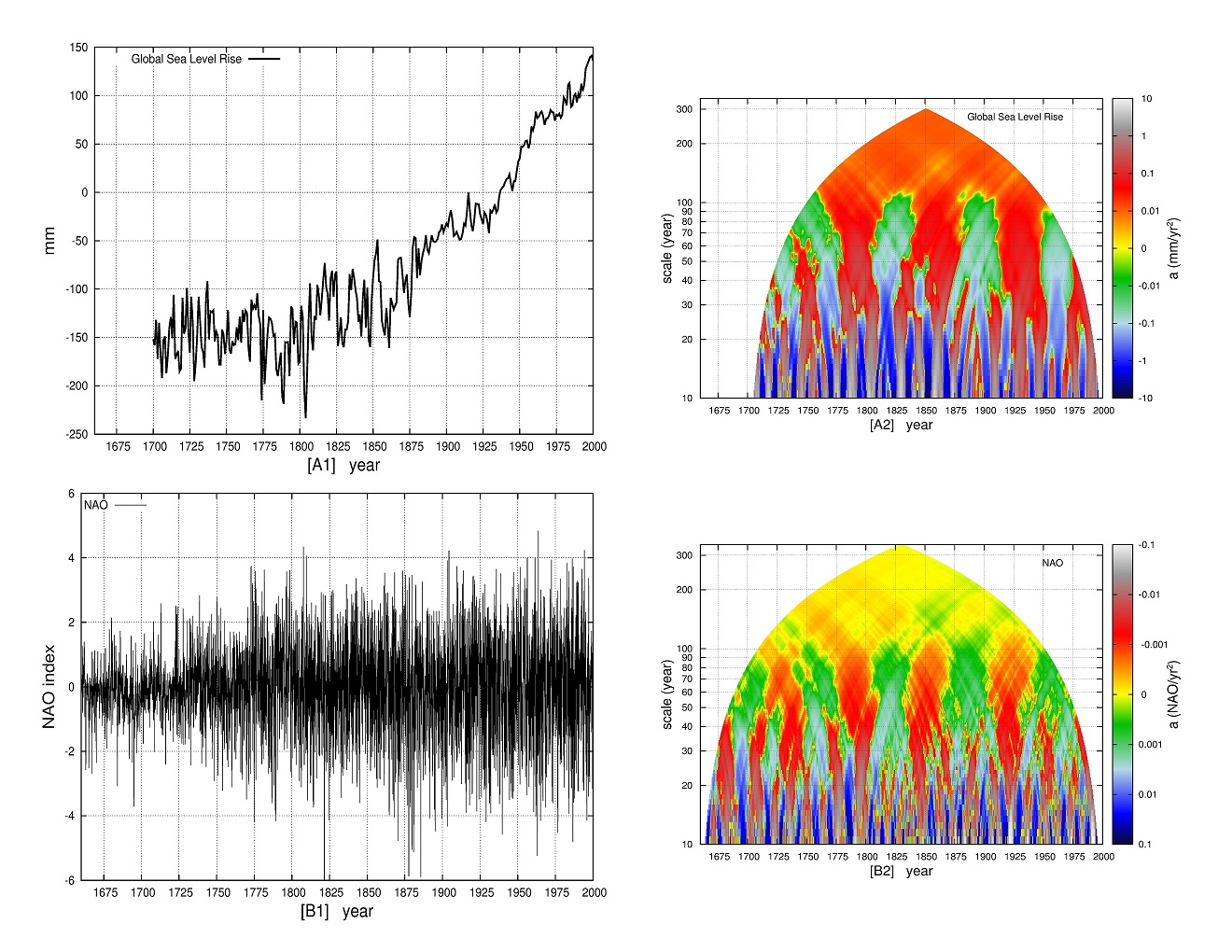
Figure 10: [A] Global sea level record (Jevrejeva et al., 2008) (left) and its MSAA colored diagram (right). [B] North Atlantic Oscillation (NAO) (Luterbacher et al., 1999, 2002) (left) and its MSAA colored diagram (right). In [B] the colors are inverted. Note the common 60-70 year oscillation since 1700 indicated by the alternating green and red regions within the 30-110 year scales.

3.2 Multi-scale rate analysis (MSRA)

The “acceleration” used in the MSAA can be substituted with other physical measures (e.g., rates, etc.) as necessary. Here a multi-scale rate analysis (MSRA) is proposed. For example, for determining the average rate, $v$, during a specific time period, the data have to be fit with a linear function of the type:

$$g(t)=v(t-t_{0})+c_{0}+H_{c}\cos(2\pi t)+H_{s}\sin(2\pi t),$$ (3)

where $v$ is the average rate in $mm/year$ during the analyzed period, and $c_{0}$is the level at $t_{0}$. The annual oscillation is added in the regression model for improved accuracy although almost no difference in the colored diagrams would be observed for tide gauge records. Once the rate values are calculated for all available time intervals and scales, they can be plotted using a colored palette diagram. Figure 8 shows the results obtained for the six tide gauge records used in the paper.

Evidently, also the rate changes and oscillates in function of the time interval and of the scale. At smaller scales (10-30 year) a large volatility is observed, and also negative rates are observed during specific periods. Extended periods with rates close to zero (green color) are observed in many records.

The color at the top of the triangles gives the average secular rate at the highest available scale, that is, for the entire available record. The following secular rate values are obtained: [A] Sydney, $v=0.63\pm 0.04$ $mm/year$; [B] Honolulu, $v=1.44\pm 0.04$ $mm/year$; [C] Fremantle, $v=1.51\pm 0.09$ $mm/year$; [D] San Diego, $v=2.04\pm 0.06$ $mm/year$; [E] New York, $v=2.99\pm 0.06$ $mm/year$; [F] Venice, $v=2.4\pm 0.1$ $mm/year$.

3.3 Multi-scale annual cycle amplitude analysis (MSACAA)

Eq. 2 contains harmonic constructors that can be used to evaluate the average amplitude and phase of the annual cycle presents in the tide gauge records. For example, for each scale and period it is possible to evaluate a total average amplitude (from minimum to maximum) with the equation:

$$H=2\sqrt{H_{c}^{2}+H_{s}^{2}}.$$ (4)

The MSACAA diagrams for the six tide gauge records are shown in Figure 9.

Also the average seasonal annual amplitude of the tide gauge records varies with the scale and the time period. In the case of Sydney, Hononulu, Fremantle and Sydney, which are within the area of influence of the Pacific Ocean, the amplitude of the annual cycle increased on average almost at all scales above 20 years from 1900 to 2000, as demonstrated by the predominantly green colors on the left side of the diagrams that slightly become yellow/red on the right side. However, the opposite pattern is observed for New York City and Venice, which are within the area of influence of the Atlantic Ocean. Thus, the analysis appears to reveal an important asymmetric and compensating dynamical evolution between the Pacific and the Atlantic oceans. Extending the analysis to additional records may clarify this issue. At smaller scales, several oscillations are observed.

4 Multisecular MSAA comparison between the global sea level record and the NAO index

Figure 10A depicts a global sea level record (Jevrejeva et al., 2008) (left) and its MSAA (right). Eq. 1 is used because the record has an annual resolution. Figure 10B depicts a reconstruction of the North Atlantic Oscillation (NAO) (Luterbacher et al., 1999, 2002) (left) and its MSAA (right). Both records cover about 300 years from 1700 to 2002 and from 1658 to 2001, respectively. In Figure 10B, which refers to the NAO index, the colors of the MSAA diagram are inverted. Note that Jevrejeva et al. (2008, figure 2) used a linear scale truncated at $\pm 0.03$ $mm/year^{2}$, while I propose to use a logarithmic scale to cover a wider and more comprehensive range of $\pm 10$ $mm/year^{2}$.

It is easy to notice that the two records present well correlated quasi 60-70 year oscillations since 1700, as indicated by the alternating green and red regions: there appear to be a small phase-lag of a few years. This result indicates that at the 30-100 year time scales the local accelerations of this global sea level record and of the NAO index are negatively correlated. Thus, in the global sea level record proposed by Jevrejeva et al. (2008) the sea level decreases when NAO is positive, that is the air pressure at the lower latitudes is high.

The following cross-correlation coefficients between the two MSAA area diagrams are found: within the 20-100 year scales, $r=-0.29$; within the 30-100 year scales, $r=-0.44$; within the 40-100 year scales, $r=-0.57$. These correlation values are highly significant.

For scales larger than 110 years up to 300 years, the sea level presents quasi uniform accelerations of about $0.01$ $mm/year^{2}$ from 1700 to 2000, as indicated by the orange color in Figure 10A2. For example, fitting the global sea level record during the 1700-2000 period gives $a=0.0092\pm 0.0004$ $mm/year^{2}$, during the preindustrial 1700-1900 period gives $a=0.0093\pm 0.0013$ $mm/year^{2}$, and during the industrial 1900-2000 period gives $a=0.010\pm 0.004$ $mm/year^{2}$. This result might also suggest that the observed background multisecular acceleration of about $0.01$ $mm/year^{2}$ has a natural origin and may be independent of the late 20th century anthropogenic warming. Indeed, the quasi-millennial solar/climate cycle observed throughout the Holocene has been in its warming phase since the 17th century, which experienced the coldest period of the Little Ice Age during the Maunder solar minimum, and may reach a maximum during the second half of 21st century (Humlum et al., 2011; Scafetta, 2012b).

Using Eq. 1 for the 1700-2002 period, the regression rate in $t_{0}=2000$ is $v_{0}=2.3\pm 0.06$ $mm/year$. If the 1700-2002 acceleration, $a=0.0092\pm 0.0004$ $mm/year^{2}$, persists during the 21th century, by extrapolating the 1700-2002 quadratic fit, the global sea level may increase by $\sim 277\pm 7$ $mm$ from 2000 to 2100.

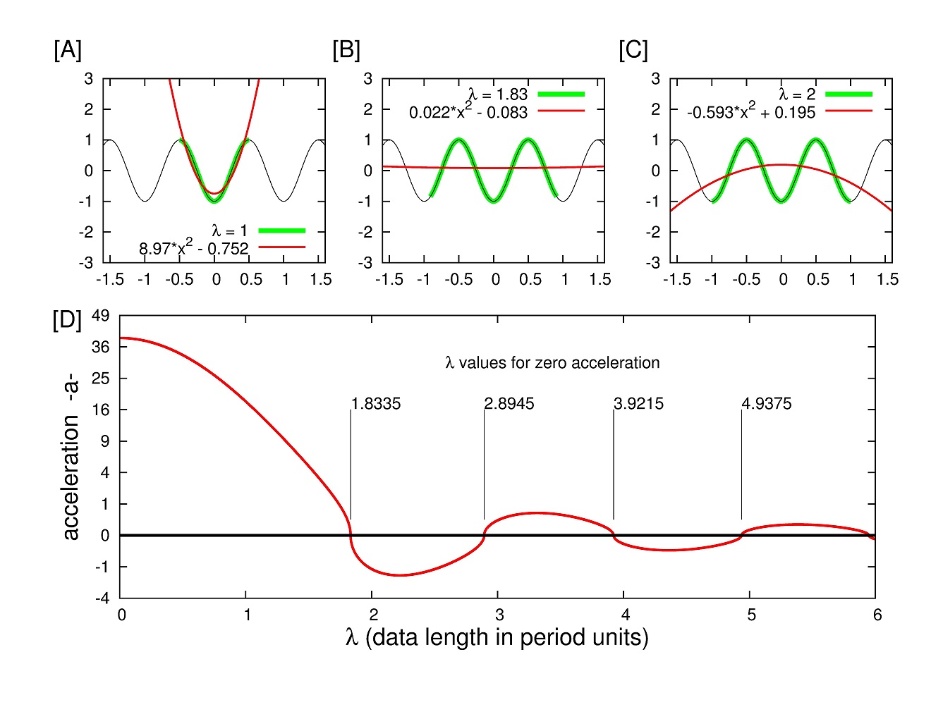
Figure 11: [A], [B] and [C] show a stationary harmonic signal (black) of unit period fit with Eq. 1 (red) within three different intervals (indicated in green) of length $\lambda=$ $1$, $1.83$ and $2$, respectively. [D] The regression acceleration coefficient in function of the record length $\lambda$. The figure demonstrates that the acceleration oscillates in function of the length interval used for the regression analysis. The values of $\lambda$ that make the acceleration $a=0$, corresponding to a fully orthogonality between the harmonic signal and the quadratic polynomial constructor are also reported.

5 Conclusion

Herein I have proposed a multi-scale dynamical analysis (MSDA) to study climatic records. The proposed technique uses graphical diagrams that greatly facilitate a comparative analysis among tide gauge records and other climatic indexes such as PDO, AMO and NAO. These records are found to be characterized by significant oscillations at the decadal and multidcadal scales up to about 110-year intervals. Within these scales both positive and negative accelerations are found if a record is sufficiently long. This result suggests that acceleration patterns in tide gauge records are mostly driven by the natural oscillations of the climate system. The volatility of the acceleration increases drastically at smaller scales such as at the bi-decadal ones.

MSAA clearly reveals a macroscopic influence of the quasi 60-year PDO and AMO oscillation in the tide gauge records, in particular for Fremantle and New York City. In fact, although during the last 40-60 years positive accelerations are typically observed in tide gauge records, as found by Sallenger et al. (2012) and by Boon (2012), also during 40-60 year intervals since the beginning of the 20th century equivalent or even higher positive accelerations are typically observed. On the contrary, at these same time scales, negative accelerations are observed during the middle of the 20th century. This pattern demonstrates the influence of a large multidecadal 60-year natural cycle, which has been found in climate and solar/astronomical records by numerous authors (e.g: Klyashtorin et al., 2009; Jevrejeva et al., 2008; Chambers et al., 2012; Scafetta, 2010, 2012a; Scafetta and Willson, 2013; Soon and Legates, 2013; Ogurtsov et al., 2002). The existence of a 60-70 year oscillation is evident in Figure 10 that shows the MSAA comparison between a global reconstruction of the sea level and of the NAO index from 1700 to 2000. The figure demonstrates that the sea level acceleration patterns during the last 60 years are not particularly anomalous relative to previous periods because they repeat quasi-periodically for three hundred years and well correlate with an independent climatic index such as the long NAO reconstruction record by Luterbacher et al. (1999, 2002).

Because of the presence of a quasi 60-year oscillation, a background secular acceleration (e.g. one that could be caused by the 20th century anthropogenic warming) can be properly evaluated only for tide gauge records longer than about 110 years, as Figure 10A2 implicitly shows. If only shorter periods are available, separating a background acceleration from a 60-year oscillation is quite difficult because the record would not be sufficiently long to determine the correct amplitude and phase of the oscillation, which are required to separate the oscillation from a background quadratic polynomial term. More precisely, if the time interval to be fitted is significantly shorter than about 2 periods of the oscillation, a quadratic polynomial constructor would be too collinear with a sinusoidal oscillation, and in collinearity cases the linear regression algorithm becomes highly unreliable. The test depicted in Figure 11 demonstrates that the minimum length that a record must have for making a quadratic polynomial constructor fully orthogonal to a sinusoidal curve is $\lambda=1.8335$ the period of the oscillation: that is, a 110-year long record is necessary for fully filtering out a 60-year periodic cycle from a background quadratic polynomial trend. In general, as Figure 11D implies, in the case of a record characterized by a 60-year cycle, using 100-year or longer records would be sufficiently fine, but using, for example, 60-year long or shorter records (e.g. as done in Sallenger et al., 2012) can be highly misleading because the quadratic fit would interpret the bending of the 60-year oscillation as a strongly accelerating trend.

When about 100-year long records are studied the evaluated average accelerations are (positively or negatively) close to zero (Church and White, 2011; Houston and Dean, 2011). Among the analyzed six tide gauge records (Sydney, Fremantle, New York, Honolulu, San Diego and Venice) two records present a slight positive secular acceleration ($\sim 0.01$ $mm/year^{2}$), while the other four records present a slight negative secular acceleration ($\sim-0.01$ $mm/year^{2}$). The 1700-2000 global sea level index proposed by Jevrejeva et al. (2008) shows an almost uniform acceleration ($\sim 0.01$ $mm/year^{2}$) at scales larger than 110 years spanning from the Little Ice Age in 1700 to modern times. Thus, it is difficult to determine whether the late 20th century anthropogenic warming had a significant effect on tide gauge records. An anthropogenic warming effect appears to be in any case too small to be clearly separated from the multidecadal and multisecular natural variability. For example, because the global sea level record proposed by Jevrejeva et al. (2008) presents an uniform secular-scale acceleration of about $\sim 0.01$ $mm/year^{2}$ since 1700, a theoretical post-1900 sea level acceleration associated to the anthropogenic warming could be constrained between $\sim 0.0$ $mm/year^{2}$ and $\sim 0.02$ $mm/year^{2}$, where the upper limit would apply in the eventuality that the natural acceleration component from 1700 to 1900 was due to a millennial oscillation that since 1900 changed inflection by turning the natural component of the acceleration into a negative value of $\sim-0.01$ $mm/year^{2}$. Indeed, the slight negative secular acceleration found in a majority of tide gauge records (Houston and Dean, 2011) may also be due to the quasi millennial oscillation typically found in numerous climatic and solar indexes throughout the Holocene, which will reach its millennium maximum during the 21st century (Humlum et al., 2011; Scafetta, 2012b).

In conclusion, at scales shorter than 100-years, the measured tide gauge accelerations are strongly driven by the natural oscillations of the climate system (e.g. PDO, AMO and NAO). At the smaller scales (e.g. at the decadal and bi-decadal scale) they are characterized by a large volatility due to significant decadal and bi-decadal climatic oscillations (Scafetta, 2009, 2010, 2012a; Manzi et al., 2012). Therefore, accelerations, as well as linear rates evaluated using a few decades of data (e.g. during the last 20-60 years) cannot be used for constructing reliable long-range projections of sea-level for the 21st century. The oscillating natural patterns need to be included in the models for producing reliable forecasts at multiple time scales. The proposed MSDA methodologies (e.g. MSAA, MSRA and MSACAA) provide a comprehensive picture to comparatively study dynamical patterns in tide gauge records. The techniques can be efficiently used for a quick and robust study of alternative climatic sequences as well.

Appendix: data

Data can be downloaded from the following web-sites:

Tide gauge records: http://www.psmsl.org/data/obtaining/

PDO: http://jisao.washington.edu/pdo/PDO.latest

AMO: http://www.esrl.noaa.gov/psd/data/correlation/amon.us.long.data

NAO: http://www.esrl.noaa.gov/psd/gcos_wgsp/Timeseries/RNAO/

Global sea level: http://www.psmsl.org/products/reconstructions/jevrejevaetal2008.php

References

- Boon (2012) Boon, J.D., 2012. Evidence of sea level acceleration at U.S. and Canadian tide stations, Atlantic Coast, North America. J. Coastal Research 28(6), 1437–1445.
- Boretti (2012) Boretti, A., 2012. Is there any support in the long term tide gauge data to the claims that parts of Sydney will be swamped by rising sea levels? Coastal Engineering 64, 161–167.
- Chambers et al. (2012) Chambers, D.P., Merrifield, M.A., and Nerem, R.S., 2012. Is there a 60-year oscillation in global mean sea level? Geophysical Research Letters 39, L18607.
- Church and White (2006) Church, J.A., White, N.J., 2006. A 20th century acceleration in global sea level rise. Geophysical Research Letters 33, L01602.
- Church and White (2011) Church, J.A., White, N.J., 2011. Sea-level rise from the late 19th to the early 21st Century. Surveys in Geophysics 32 (4–5), 585–602.
- Chylek et al. (2011) Chylek, P., Folland, C.K., Dijkstra, H.A., Lesins, G., and Dubey, M.K., 2011. Ice-core data evidence for a prominent near 20 year time-scale of the Atlantic Multidecadal Oscillation. Geophysical Research Letters 38, L13704.
- Douglas (1992) Douglas, B. C., 1992. Global sea level acceleration. J. Geophys. Res. 97, 12699-12706.
- Dean and Houston (2013) Dean, R.G., Houston, J.R., 2013. Recent sea level trends and accelerations: Comparison of tide gauge and satellite results. Coastal Engineering, 75, 4–9.
- Houston and Dean (2011) Houston, J.R., Dean, R.G., 2011. Sea-Level Acceleration Based on U.S. Tide Gauges and Extensions of Previous Global-Gauge Analyses. Journal of Coastal Research 27, 409–417.
- Humlum et al. (2011) Humlum, O., Solheim, J.-K., Stordahl, K., 2011. Identifying natural contributions to late Holocene climate change. Global and Planetary Change 79, 145–156.
- Hunter and Brown (2013) Hunter, J.R., Brown, M.J.I, 2013. Discussion of Boretti, A., ‘Is there any support in the long term tide gauge data to the claims that parts of Sydney will be swamped by rising sea levels?’, Coastal Engineering, 64, 161–167, June 2012. Coastal Engineering 75, 1–3.
- IPCC (2007) IPCC: Solomon, S., et al. (eds) in Climate Change 2007: The Physical Science Basis.Contribution of Working Group I to the Fourth Assessment Report of the Intergovernmental Panel on Climate Change, (Cambridge University Press, Cambridge, 2007).
- Jevrejeva et al. (2008) Jevrejeva, S., et al., 2008. Recent global sea level acceleration started over 200 years ago? Geophysical Research Letters 35, L08715.
- Kennedy et al. (2011a) Kennedy, J. J., Rayner, N. A., Smith, R. O., Saunby, M., Parker, D. E., 2011a. Reassessing biases and other uncertainties in sea-surface temperature observations since 1850 part 1: measurement and sampling errors. J. Geophys. Res., 116, D14103.
- Kennedy et al. (2011b) Kennedy, J. J., Rayner, N. A., Smith, R. O., Saunby, M. and Parker, D. E., 2011b. Reassessing biases and other uncertainties in sea-surface temperature observations since 1850 part 2: biases and homogenisation. J. Geophys. Res., 116, D14104, doi:10.1029/2010JD015220
- Klyashtorin et al. (2009) Klyashtorin, L.B., Borisov, V., Lyubushin, A., 2009. Cyclic changes of climate and major commercial stocks of the Barents Sea. Marine Biology Research 5, 4-17.
- Knudsen et al. (2011) Knudsen, M.F., Seidenkrantz, M-S., Jacobsen, B.H., Kuijpers, A., 2011. Tracking the Atlantic Multidecadal Oscillation through the last 8,000 years. Nature Communications 2, 178.
- Kobashi et al. (2010) Kobashi, T., Severinghaus, J., Barnola, J.-M., Kawamura, K., Carter, T., Nakaegawa, T., 2010. Persistent multi-decadal Greenland temperature fluctuation through the last millennium. Climate Change 100, 733-756.
- Levermann et al. (2005) Levermann, A., Griesel, A., Hofmann, M., Montoya, M., Rahmstorf, S., 2005. Dynamic sea level changes following changes in the thermohaline circulation. Clim. Dynam. 24, 347–354.
- Loehle and Scafetta (2011) Loehle, C., N. Scafetta, N., 2011. Climate Change Attribution Using Empirical Decomposition of Climatic Data. The Open Atmospheric Science Journal 5, 74-86.
- Luterbacher et al. (1999) Luterbacher, J., Schmutz, C., Gyalistras, D., Xoplaki, E., Wanner, H., 1999. Reconstruction of monthly NAO and EU indices back to AD 1675. Geophys. Res. Lett. 26, 2745-2748.
- Luterbacher et al. (2002) Luterbacher, J., Xoplaki, E., Dietrich, D., Jones, P. D., Davies, T. D., Portis, D., Gonzalez-Rouco, J. F., von Storch, H., Gyalistras, D., Casty, C., and Wanner, H., 2002. Extending North Atlantic Oscillation Reconstructions Back to 1500. Atmos. Sci. Lett., doi:10.1006/asle.2001.0044.
- Mantua et al. (1997) Mantua, N. J., Hare, S. R., Zhang, Y., Wallace, J. M., Francis, R. C., 1997. A Pacific Interdecadal Climate Oscillation with Impacts on Salmon Production. Bull. Amer. Meteor. Soc. 78, 1069–1079.
- Manzi et al. (2012) Manzi V., Gennari, R., Lugli, S., Roveri, M., Scafetta, N., Schreiber, C., 2012. High-frequency cyclicity in the Mediterranean Messinian evaporites: evidence for solar-lunar climate forcing. Journal of Sedimentary Research 82, 991-1005.
- Mazzarella and Scafetta (2012) Mazzarella, A., Scafetta, N., 2012. Evidences for a quasi 60-year North Atlantic Oscillation since 1700 and its meaning for global climate change. Theoretical and Applied Climatology 107, 599-609.
- Mörner (1989) Mörner, N.-A., 1989. Changes in the Earth’s rate of rotation on an El Nino to century basis. In: Geomagnetism and Paleomagnetism ( F.J. Lowes et al., eds), 45-53, Kluwer Acad. Publ.
- Mörner (1990) Mörner, N.-A., 1990. The Earth’s differential rotation: hydrospheric changes. Geophysical Monographs, 59, 27-32, AGU and IUGG.
- Mörner (2010) Mörner, N.-A., 2010. Some problems in the reconstruction of mean sea level and its changes with time. Quaternary International 221 (1-2), 3-8.
- Ogurtsov et al. (2002) Ogurtsov, M. G., Nagovitsyn, Y. A., Kocharov, G. E., Jungner, H., 2002. Long-period cycles of the Sun’s activity recorded in direct solar data and proxies. Solar Physics 211, 371-394.
- Parker (2012a) Parker, A., 2012a. Oscillations of sea level rise along the Atlantic coast of North America north of Cape Hatteras. Natural Hazards 65, 991–997.
- Parker (2012b) Parker, A., 2012b. Sea level trends at locations of the United States with more than 100 years of recording. Natural Hazards 65, 1011–1021.
- Parker (2013) Parker, A., 2013. Natural oscillations and trends in long-term tide gauge records from the Pacific. Pattern Recogn. Phys., 1, 1-13.
- PSMLS (2013) Permanent Service for Mean Sea Level (PSMSL), 2013. Tide Gauge Data. The records were downloaded during Feb 2013.
- Sallenger et al. (2012) Sallenger Jr., A.H., Doran, K.S., Howd, P.A., 2012. Hotspot of accelerated sea-level rise on the Atlantic coast of North America. Nature Climate Change 2, 884-888.
- Scafetta (2009) Scafetta N., 2009. Empirical analysis of the solar contribution to global mean air surface temperature change. Journal of Atmospheric and Solar-Terrestrial Physics 71, 1916-1923.
- Scafetta (2010) Scafetta, N., 2010. Empirical evidence for a celestial origin of the climate oscillations and its implications. Journal of Atmospheric and Solar-Terrestrial Physics 72, 951-970.
- Scafetta (2012a) Scafetta N., 2012a. Testing an astronomically based decadal-scale empirical harmonic climate model versus the IPCC (2007) general circulation climate models. Journal of Atmospheric and Solar-Terrestrial Physics 80, 124-137.
- Scafetta (2012b) Scafetta N., 2012b. Multi-scale harmonic model for solar and climate cyclical variation throughout the Holocene based on Jupiter-Saturn tidal frequencies plus the 11-year solar dynamo cycle. Journal of Atmospheric and Solar-Terrestrial Physics 80, 296-311.
- Scafetta and Willson (2013) Scafetta, N., Willson, R. C., 2013. Planetary harmonics in the historical Hungarian aurora record (1523–1960). Planetary and Space Science 78, 38-44.
- Schlesinger and Ramankutty (1994) Schlesinger, M. E., Ramankutty, N., 1994. An oscillation in the global climate system of period 65-70 years. Nature 367, 723-726.
- Soon and Legates (2013) Soon, W., Legates, D. R., 2013. Solar irradiance modulation of Equator-to-Pole (Arctic) temperature gradients: Empirical evidence for climate variation on multi-decadal timescales. J. of Atmospheric and Solar-Terrestrial Physics 93, 45-56.
- Woodworth (1990) Woodworth, P. L., 1990. A search for accelerations in records of European mean sea-level. Int. J. Climatol. 10, 129-143.
- Woodworth and Player (2003) Woodworth, P. L., Player, R., 2003. The Permanent Service for Mean Sea Level: an update to the 21st century. Journal of Coastal Research, 19, 287-295.
- Woodworth et al. (2009) Woodworth, P. L., White, N. J. Jevrejeva, S., Holgate, S. J., Church, J. A., Gehrels, W. R., 2009. Evidence for the accelerations of sea level on multi-decade and century timescales. Int. J. Climatol. 29, 777-789.