Soft computing-based calibration of microplane M4 model parameters: Methodology and validation

Abstract

Constitutive models for concrete based on the microplane concept have repeatedly proven their ability to well-reproduce non-linear response of concrete on material as well as structural scales. The major obstacle to a routine application of this class of models is, however, the calibration of microplane-related constants from macroscopic data. The goal of this paper is two-fold: (i) to introduce the basic ingredients of a robust inverse procedure for the determination of dominant parameters of the M4 model proposed by Bažant and co-workers in [5] based on cascade Artificial Neural Networks trained by Evolutionary Algorithm and (ii) to validate the proposed methodology against a representative set of experimental data. The obtained results demonstrate that the soft computing-based method is capable of delivering the searched response with an accuracy comparable to the values obtained by expert users.

Department of Mechanics, Faculty of Civil Engineering

Czech Technical University in Prague

Thákurova 7, 166 29 Prague, Czech Republic

Dedicated to Professor Zdeněk Bittnar in occasion of his 70th birthday.

Keywords: computational simulation of concrete, microplane model M4, inverse analysis, neural networks, global sensitivity analysis, evolutionary algorithm.

1 Introduction

Despite long-term use of concrete in civil engineering industry, development of an exhaustive constitutive model for concrete still remains in the focus of engineering materials science. The difficulty in constitutive modeling is directly linked to the complexity of the material itself: the quasi-brittle response of concrete as seen on macroscale is a consequence of non-linear interactions of its numerous constituents over a wide range of lengthscales. As a result, a formulation of a concise model reproducing experimental data while satisfying the constraints of continuum thermodynamics is far from being trivial.

One of the most successful modeling approaches stems from the microplane concept, in which the response of a macroscopic material point results from contributions of planes of all possible orientations, see e.g. [12, Chapter 25]. The potential of this modeling paradigm was perhaps best demonstrated by the M4 model for concrete introduced by Bažant and co-workers [5], which has repeatedly shown its capacity to realistically reproduce response of complex three-dimensional structures under general loading conditions. In addition, an efficient parallelization strategy [27] or model adaptivity [32] were proposed to compensate for an increased computational cost of the microplane models with respect to traditional approaches.

The major strength of the microplane concept – the implicit format of the macroscopic constitutive law – is however closely linked to its major obstacle: the model constants are directly linked to the microplane level and as such are difficult to interpret and identify from experiments performed at the macroscopic level. In the particular case of the M4 model for concrete, Caner and Bažant proposed in [7] a heuristic sequence of experiments to calibrate adjustable parameters of the model. Nevertheless, the procedure is still based on a hand-fitting procedure, thereby requiring an expert user or a tedious trial-and-error calibration procedure. To relax this constraint, hereafter we introduce a robust automated procedure for the calibration of the M4 model constants.

An independent certificate to the non-trivial character of the automated M4 model calibration is provided by difficulties associated with the selection of an appropriate class of optimization algorithms to solve the resulting optimization problem based on the minimization of the objective function. Following the well-established classification of the inverse algorithms introduced by Mahnken in [21], the most efficient solution strategies are typically based on gradient-based optimization methods. Although several successful applications to quasi-brittle materials have been reported in the past, e.g. [22], they cannot be applied in the microplane setting since a closed-form tangent is not available, resulting in a non-smooth objective function.

The requirements of smoothness can be relaxed by resorting to the evolutionary algorithms. Although these methods were successfully applied to inverse analysis of a variety of engineering constitutive models, see e.g. [16] and references therein, their extremely high demand for a number of function calls combined with computational cost of the microplane model prohibits their use even in the parallel environment, see [20].

To reduce the high computational cost of the resulting problem, one may reconcile oneself to an approximate solution by resorting to an inexpensive approximation of the quantity of interest. At this step, network-type approximations are frequently employed due to their simplicity and extremely high degree of flexibility. In general, two complementary strategies to an approximate identification problem can be distinguished [16]: (i) the forward mode, where either the systems’ response or the objective function itself is to be replaced and (ii) the inverse mode where an approximate map from measurable quantities to model parameters is to be established. The former model was, e.g., successfully applied to complex geotechnical problems [30] or to an identification of parameters for damage-plasticity models from large-scale tests by Kučerová et. al [17]. Extensions towards the microplane case, however, suffer from the fact that an accurate representation of the load-displacement curve or the objective function itself still requires a significant number of degrees of freedom, which, when to be determined reliably, leads to an excessive number of simulations. Moreover, a high accuracy of approximations is usually needed to obtain the identified parameters with an acceptable accuracy [17]. Therefore, high computational costs make it difficult to successfully implement this strategy for the microplane identification problem.

The inverse identification mode, on the other hand, is substantially more computationally efficient and is being widely used in a wide range of material calibration problems, see again [16] and references therein. The critical issue in this case remains the inherent ill-conditioning of the problem, especially when determining a parameter with a low sensitivity for the executed experiment. This fact was exactly the reason for the failure of our early applications of the inverse mode to the microplane identification problem, see [9] for a particular illustration of this issue. Fortunately, efficient small-size procedures are currently available to estimate the sensitivity of a particular parameter and, as demonstrated by our recent work [14], present a natural choice to identify the model parameters.

In the current work, we introduce a well-defined procedure for the identification of material parameters for M4 microplane model. The procedure itself is based on work by Novák and Lehký [25] and has been successfully verified against artificially generated sets of data in [19]. Here, we present an independent validation and comparison with expert user guesses.

The remainder of the paper is organized as follows. The next section is devoted to the short introduction and a description of our implementation of M4 microplane model. The inverse mode of parameters’ estimation is presented next with an emphasis put on artificial neural networks and their training. The main part is describing the methodology behind the identification of all pertinent M4 model parameters. To get reliable results, two “tricks” are used. The first one is usage of cascade neural networks [33] where some already identified parameters serve as inputs to later stages of identification. The second one is the combination of two models for closely interacting parameters. The combination defines a nonlinear equation which can be easily solved numerically. The main part is – according to M4 authors – divided to three sections corresponding to the tests needed for M4 parameters estimation: the uniaxial, hydrostatic and triaxial tests. In the closing section, the presented text is accompanied by the analysis of the computational demands which present the main drawbacks of the presented methodology.

2 COMPUTATIONAL MODEL

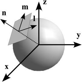
In contrary to traditional approaches to constitutive modeling, which build on description via second-order strain and stress tensors at individual points in the $(x,y,z)$ coordinate system, the microplane approach builds the descriptions on planes of arbitrary spatial orientations – so-called microplanes, related to a macroscopic point, see Figure 1. This allows to formulate constitutive equations in terms of stress and strain vectors in the coordinate system $(\mathbf{l},\mathbf{m},\mathbf{n})$ associated with a microplane oriented by a normal vector $\mathbf{n}$. The general procedure of evaluation of a strain-driven microplane model response for a given “macroscopic” strain tensor $\mbox{\boldmath$\varepsilon$}(\mathbf{x})$ can be described as follows: (i) for a given microplane orientation $\mathbf{n}$ normal “macroscopic” strain tensor $\mbox{\boldmath$\varepsilon$}(\mathbf{x})$ is projected onto the normal “microstrain” vector $\mathbf{\varepsilon}(\mathbf{n})$ and the shear microstrains $\mathbf{\varepsilon}(\mathbf{m})$ and $\mathbf{\varepsilon}(\mathbf{l})$, (ii) the normal and shear microstresses $\mathbf{\sigma}(\mathbf{n}),\mathbf{\sigma}(\mathbf{m})$ and $\mathbf{\sigma}(\mathbf{l})$ are evaluated using microplane constitutive relations, (iii) the “macroscopic” stress tensor $\mbox{\boldmath$\sigma$}(\mathbf{x})$ is reconstructed from the microscopic ones using the principle of virtual work, see, e.g., [12, Chapter 25] for more details. In the particular implementation, 28 microplanes with a pre-defined orientation on the unit hemisphere are used to evaluate the response of the model.

Figure 1: Concept of microplane modeling

To close the microplane model description, the appropriate microplane constitutive relation must be provided to realistically describe material behavior. The model examined in the current work is the microplane model M4 [5]. The model uses volumetric-deviatoric split of the normal components of the stress and strain vectors, treats independently shear components of a microplane and introduces the concept of “boundary curves” to limit unrealistically high values predicted by earlier version of the model. As a result, the strain-to-stress map $\mbox{\boldmath$\varepsilon$}(\mathbf{x})\mapsto\mbox{\boldmath$\sigma$}(\mathbf{x})$ is no longer smooth, which complicates the formulation of consistent tangent stiffness matrix [27] and, subsequently, gradient-based approaches to material model parameters identification.

In overall, the microplane model M4 needs seven parameters to describe a certain type of concrete, namely: Young’s modulus $E$, Poisson’s ratio $\nu$, and other five parameters ($k_{1}$, $k_{2}$, $k_{3}$, $k_{4}$, $c_{20}$), which do not have a simple physical interpretation, and therefore it is difficult to determine their values from experiments. The only information available in the open literature are the bounds shown in the Table 1.

Parameter		Bounds
$E$	$\in$	$\langle 20.0,50.0\rangle$ GPa
$\nu$	$\in$	$\langle 0.1,0.3\rangle$
$k_{1}$	$\in$	$\langle 0.00008,0.00025\rangle$
$k_{2}$	$\in$	$\langle 100.0,1000.0\rangle$
$k_{3}$	$\in$	$\langle 5.0,15.0\rangle$
$k_{4}$	$\in$	$\langle 30.0,200.0\rangle$
$c_{20}$	$\in$	$\langle 0.2,5.0\rangle$

Table 1: Bounds for the microplane model parameters

In the present work, the computational model of a structure is provided by the object-oriented C++ finite element code OOFEM 1.5 [29, 28]. Spatial discretization is performed using linear brick elements with eight integration points. The arc-length method with elastic stiffness matrix is used to determine the load-displacement curve related to the analyzed experiment.

3 PARAMETER IDENTIFICATION METHODOLOGY

The problem of model parameters identification starts by the design and realization of a suitable experiment $E({\bf x}^{\mathrm{E}})={\bf y}^{\mathrm{E}}$, which connects material properties ${\bf x}^{\mathrm{E}}$ with some observable quantities ${\bf y}^{\mathrm{E}}$ under some given loading conditions. Then we assume to have an appropriate numerical model $M({\bf x}^{\mathrm{M}})={\bf y}^{\mathrm{M}}$ approximating the experiment in an efficient and accurate way. The goal is then to estimate the values of the model parameters ${\bf x}^{\mathrm{M}}$ minimizing the difference between the model outputs ${\bf y}^{\mathrm{M}}$ and observed data ${\bf y}^{\mathrm{E}}$.

As it was mentioned in introduction, many different identification methodologies are available in literature. Nevertheless, only a limited number of them were reliably verified. As the authors of [3] introduced terms verification and validation for numerical models of physical events, we will follow here the definition of those terms in the field of parameters identification presented in [16]:

• Verification: The process of determining whether the identification method is able to re-find the model parameters ${\bf x}^{\mathrm{M}}$ from the outputs ${\bf y}^{\mathrm{ref}}$ of the reference simulation done for any choice of original inputs ${\bf x}^{\mathrm{ref}}$.

• Validation: The process of determining whether the identification method is able to find the model parameters ${\bf x}^{\mathrm{M}}$ corresponding to the experimental outputs ${\bf y}^{\mathrm{E}}$.

In this paper, we focus on an inverse mode of an identification strategy, which was already verified for parameters identification on microplane model [19] and we would like to extend this work by validation on experimental data. Therefore, we just briefly review the main principles of the applied methodology and an interested reader can find more information in [19].

The methodology assumes an existence of an inverse relationship between model outputs ${\bf y}^{\mathrm{M}}$ and model inputs ${\bf x}^{\mathrm{M}}$, i.e. there is an inverse model $M_{\mathrm{inv}}$ associated to the model $M$, which fulfils ${\bf x}^{\mathrm{M}}=M_{\mathrm{inv}}({\bf y}^{\mathrm{M}})$. Generally, this inverse model does not need to exist. Nevertheless, we assume that the inverse model can be found sufficiently precise on some closed subdomain of the parameter space. Next, we will limit our attention to an approximation of the inverse relationship, not its exact description. A quality of this approximation is easy to measure since a pair ${\bf x}$, ${\bf y}$ obtained using inverse model $M_{\mathrm{inv}}(\cdot)$ should also fulfill the forward model relation $M(\cdot)$. Final usage of this methodology is trivial because a desired value ${\bf x}^{\mathrm{M}}$ can be simply obtained as ${\bf x}^{\mathrm{M}}=M_{\mathrm{inv}}({\bf y}^{\mathrm{E}})$.

The main advantage is clear. If an inverse relationship is established, then the retrieval of desired inputs is a matter of seconds even if executed repeatedly. This can be utilized for frequent identification of one model. On the contrary, the main disadvantages are an exhausting search for the inverse relationship, the existence problems for the whole search domain and inability to solve the problem of several global optima.

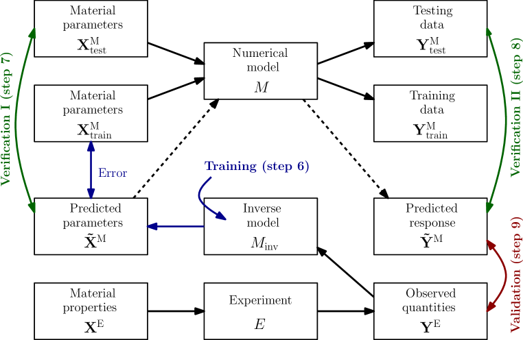
The presented identification strategy is based on an approximation of inverse relation using an artificial layered neural network (ANN), which is known as a very general and robust approximation tool. Individual steps of the identification strategy involve:

Step 1

Setup of an experimental test used for the identification procedure and storing the observed quantities ${\bf y}^{\mathrm{E}}$.

Step 2

Randomization of input parameters. Input data are typically assumed to be random variables uniformly distributed on a given interval, which roughly lead to equally distributed precision of an ANN over the parameter domain. Of course, any other distribution for parameters is admissible to improve the ANN’s accuracy e.g. in the vicinity of particular parameter values. A representative set of input vectors ${\bf X}^{\mathrm{M}}_{\mathrm{train}}=\left[{\bf x}_{1}^{\mathrm{M}},{\bf x}_{2}^{\mathrm{M}},\dots,{\bf x}_{n_{\mathrm{train}}}^{\mathrm{M}}\right]$ is carefully chosen for ANN training following the design of experiments methodology [23]. Another set of input vectors ${\bf X}^{\mathrm{M}}_{\mathrm{test}}=\left[{\bf x}_{1}^{\mathrm{M}},{\bf x}_{2}^{\mathrm{M}},\dots,{\bf x}_{n_{\mathrm{test}}}^{\mathrm{M}}\right]$ is randomly chosen for ANN testing. $n_{\mathrm{train}}$ and $n_{\mathrm{test}}$ denote the number of training and testing samples, respectively.

Step 3

Training and testing data sets preparation. The computational model $M$ is applied to simulate the experiment $E$ for all training and testing input vectors in order to obtain corresponding output vectors ${\bf Y}^{\mathrm{M}}_{\mathrm{train}}=\left[{\bf y}_{1}^{\mathrm{M}},{\bf y}_{2}^{\mathrm{M}},\dots,{\bf y}_{n_{\mathrm{train}}}^{\mathrm{M}}\right]$ and ${\bf Y}^{\mathrm{M}}_{\mathrm{test}}=\left[{\bf y}_{1}^{\mathrm{M}},{\bf y}_{2}^{\mathrm{M}},\dots,{\bf y}_{n_{\mathrm{test}}}^{\mathrm{M}}\right]$, respectively, where ${\bf y}_{i}^{\mathrm{M}}=M({\bf x}^{\mathrm{M}}_{i})$.

Step 4

Global sensitivity analysis using the training simulations. This provides us with relevant model parameters which can be reliably identified from the computational simulation. Usually this step is performed by calculation the correlation between inputs ${\bf X}^{\mathrm{M}}_{\mathrm{train}}$ and outputs ${\bf Y}^{\mathrm{M}}_{\mathrm{train}}$.

Step 5

Definition of the topology of an ANN used for the identification procedure.

Step 6

Training of the ANN, i.e. developing $M_{\mathrm{inv}}$. Usually an optimization algorithm is needed to appropriately setup values of synaptic weights ${\bf w}$ of the ANN by minimizing the error function $E({\bf w})=\|(M_{\mathrm{inv}}({\bf Y}^{\mathrm{M}}_{\mathrm{train}},{\bf w})-{\bf X}^{\mathrm{M}}_{\mathrm{train}}\|$.

Step 7

Verification I of the ANN with respect to the computational model. This step is usually performed by comparing the ANN’s prediction of model input parameters ${\bf{\tilde{X}}}^{\mathrm{M}}_{\mathrm{test}}=M_{\mathrm{inv}}({\bf Y}^{\mathrm{M}}_{\mathrm{test}},{\bf w})$, with the original one ${\bf X}^{\mathrm{M}}_{\mathrm{test}}$ for unseen testing (or reference) data.

Step 8

Verification II of the ANN with respect to the computational model. In this step, a computational model should be evaluated for predicted values ${\bf{\tilde{X}}}^{\mathrm{M}}_{\mathrm{test}}$ in order to obtain corresponding model outputs ${\bf{\tilde{Y}}}^{\mathrm{M}}_{\mathrm{test}}$. Then the outputs ${\bf{\tilde{Y}}}^{\mathrm{M}}_{\mathrm{test}}$ are compared with the original ones ${\bf Y}^{\mathrm{M}}_{\mathrm{test}}$. This step is not necessary, but is utmost recommended.

Step 9

Validation of the ANN with respect to the experiment. The trained ANN is evaluated for experimental data ${\bf y}^{\mathrm{E}}$ in order to obtain corresponding input values ${\bf{\tilde{x}}}^{\mathrm{E}}=M_{\mathrm{inv}}({\bf y}^{\mathrm{E}})$ of the computation model $M$. The model $M$ is then evaluated for obtained inputs ${\bf{\tilde{x}}}^{\mathrm{E}}$ and results ${\bf{\tilde{y}}}^{\mathrm{E}}=M({\bf{\tilde{x}}}^{\mathrm{E}})$ are compared with original measured data ${\bf y}^{\mathrm{E}}$.

For clarity, the scheme of such identification procedure is displayed in Figure 2.

Figure 2: Scheme of inverse analysis procedure

3.1 NEURAL NETWORKS ARCHITECTURE

Multilayer neural networks became very popular as an universal approximation tool [2]. The ANN is composed of a set of simple operational units - neurons. Each neuron is represented by an activation function, which defines the relation between an input and output value of the neuron. In the multi-layered neural network, neurons are ordered into layers, where outputs of neurons from one layer multiplied by appropriate synaptic weights serve as input values for a neuron in the next layer, see e.g. [6] for more details.

When looking for a suitable neural network, two non-trivial tasks must be solved [34]: (a) a choice of an appropriate architecture and (b) a search for optimal values of synaptic weights, i.e. so-called training of a neural network. In our applications, we follow the premise that only three layers with enough hidden neurons are sufficient to describe any relation [8], therefore only three layers are used in our computations. Another premise used is that it is easier to train several networks with one output value than one complex network with several outputs [13]. Hence, one neural network is trained for each model parameter and the inverse model is then composed by a set of simple ANNs.

Another trick used in our computations is a cascade neural network. Here, a sequential way of identification of the individual inputs $x_{i}$ is utilized to increase the prediction abilities of the ANN-based methodology by reducing the complexity of the approximated relationship. The predictions of some parameters identified in the preceding steps are assumed as known and serve as inputs during the development of inverse models in following steps. Several applications of this methodology to parameters identification are presented e.g. in [33].

Finally, a number of input neurons that corresponds to the number of relevant observable quantities should be selected. Since in many engineering problems, measurements are represented by single or several curves usually discretized into discrete points, a number of observed quantities is often very large. Therefore, a global sensitivity analysis is applied to choose only quantities important for a particular model parameter to be identified [25]. A number of neurons in hidden layer is determined by consecutively increasing their number taking the over-training and under-training issues into account. Particularly, a goal is to find a trade-off between errors in prediction for training and testing data, respectively.

3.2 NEURAL NETWORK TRAINING

Once the architecture of the ANN is chosen, the training process can start. The most famous training algorithm still remains a relatively simple backpropagation, especially because of its simple interpretation and implementation. As the name suggests, the error in prediction of the output layer is propagated back to previous layers and according to an error’s value, synaptic weights are updated. From the optimization point of view, it is a gradient-based algorithm, which suffers from premature convergence.

Therefore, GRADE evolutionary algorithm extended by a niching strategy CERAF is used here as a more robust optimization algorithm. This algorithm was derived from its predecessor SADE algorithm, which provided better results in ANN training against the back-propagation as was presented in [9]. GRADE is a population-based real-coded algorithm consisting of three genetic operators, which are applied to a set of solutions. Particularly, it involves mutation, differential cross-over and inverse tournament selection. CERAF is a multistart strategy enhanced with memory that increases the ability of a population-based algorithm to escape from local extremes. An interested reader can find more details about both methods in [16] or [18, 15], where C++ and MATLAB implementations are available. For information on other possible training algorithms see e.g. [13] or a review [34].

4 EXPERIMENTAL VALIDATION

Following the heuristic calibration procedure suggested in [7], we examine three specific experimental tests: (i) uniaxial compression, (ii) hydrostatic test and (iii) triaxial test. Advantage of these tests is their simplicity and availability in most experimental facilities. Moreover, authors in [7] claim that these experiments are sufficient to determine all parameters of the microplane model M4. The results presented in this section can be understood as a verification of this claim.

In our previous contribution [19], we have shown that the proposed methodology is able to identify all parameters from computer-simulated curves. To demonstrate the applicability of the proposed procedure, a real experiment should be examined. Since the measurements from different loading tests are obtained for different concretes, this section does not represent a validation of proposed identification strategy in general, but only the validation of application of particular inverse models.

Each neural network is obtained by the procedure described previously. More precisely, a fully connected three-layer perceptron with bias neurons is applied to map discrete values from stress-strain diagrams to microplane model parameters. Log-sigmoid functions are considered as activation functions in all neurons. In all cases studied in this work, 60 training samples are generated by Latin Hypercube Sampling method and optimized by Simulated Annealing in order to minimize the correlation among all samples [25]. Those two methods are implemented in FREET software [26] that has been used. Next, 10 testing samples are obtained for random parameters from given bounds. Relevant values selected from stress-strain diagram as ANN’s inputs are chosen by hand with respect to the results of global sensitivity analysis. Here, the Pearson product-moment correlation coefficient [11] is evaluated between the discrete values of stresses (or strains) and corresponding values of microplane model parameters. For the ANN training the GRADE algorithm supported by CERAF strategy is used and calculation is stopped after 1,000,000 iterations of the algorithm. Finally, all three following compression tests are performed on the cylinders with a radius equal to 75 mm and the height of 300 mm.

4.1 UNIAXIAL COMPRESSION TEST

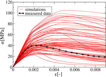
Experimental data are taken from [7, Figure 1a]. Note that the original source comes from [31]. A suite of 70 training and testing simulations and the resulting bundle of curves together with the experimental data is shown in Figure 3a.

(a)	(b)

Figure 3: Bundle of curves of uniaxial compression test simulation with experimental data for varying (a) all parameters and (b) only the constant $c_{20}$.

Only for illustrative purposes, the evolution of global sensitivity during the loading process (horizontal axis) is depicted in Figure 4a and is omitted for other two tests. The results indicate that the most sensitive parameters are Young’s modulus $E$, the coefficient $k_{1}$ and, for the later stages of loading, the coefficient $c_{20}$. Therefore, one can expect that only these parameters can be reliably identified from this test. Poisson’s ratio $\nu$ can be also identified from this type of experiment, but only if lateral deformation is measured.

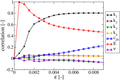(a)	(b)

Figure 4: Sensitivity analysis for uniaxial compression test: (a) evolution during the loading process and (b) peak coordinates [$\epsilon_{\mathrm{peak}}$,$\sigma_{\mathrm{peak}}$] of stress-strain curves.

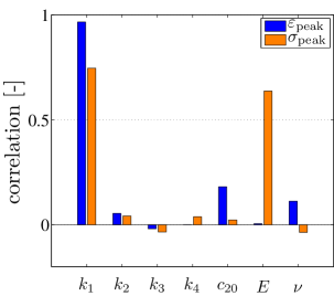
Moreover, the impact of individual parameters on a position of a peak of stress-strain curves is computed. The results of a sensitivity analysis using Pearson’s product moment correlation coefficient of peak coordinates [$\epsilon_{\mathrm{peak}}$,$\sigma_{\mathrm{peak}}$] are plotted in Fig 4b. Results indicate particularly strong influence of the $k_{1}$ parameter, which promise its reliable determination.

Based on the results of sensitivity analysis, the neural network training can be performed using a nested strategy of cascade neural networks. First, Young’s modulus $E$ with sensitivity $\approx 1$ in the initial stage is easily identified. To this end, the following ANN’s inputs are chosen: the values of stresses $\sigma_{[\hat{\epsilon}]}$, where $\hat{\epsilon}$ is a particular level of deformation with extremal Pearson’s correlation coefficient, here the starting of the loading curve, particularly $\hat{\epsilon}=0.0005;0.001$ and $0.0015$, respectively. The hidden layer contains two neurons only; the output layer consists of one neuron corresponding to the predicted value of Young’s modulus $E$, see also notation used in Table 2. Similar approach is used for $k_{1}$ parameter with the architecture described in Table 2. Note the usage of Young’s modulus $E$ estimation from the previous ANN. Errors for both ANN’s predictions are then listed in Table 3.

Parameter	Topology	Inputs
$E$	$3+2+1$	$\sigma_{[0.0005]},\sigma_{[0.001]},\sigma_{[0.0015]}$
$k_{1}$	$5+3+1$	$\sigma_{[0.0025]},\sigma_{[0.009]},\epsilon_{\mathrm{peak}},\sigma_{\mathrm{peak}}$, prediction of $E$

Table 2: Topology of neural networks for uniaxial compression test.

Parameter	Training data		Testing data
	Maximal error	Average error	Maximal error	Average error
$E$	1.97	1.01	1.50	0.81
$k_{1}$	2.68	1.57	2.63	1.50

Table 3: Errors in ANN’s prediction relative to the size of admisible domain given for the parameters in [%].

Next, the trained neural networks were applied on measured data and the following values were obtained: $E=36057$ MPa and $k_{1}=0.000196$, while the M4 authors suggest in [7] $E=32173$ MPa and $k_{1}=0.000165$.

Since the lateral deformation is missing in measured data, Poison’s ratio cannot be identified. Its value is chosen according to microplane authors’ recommendations $\nu=0.2$. According to sensitivity analysis, other parameters should not be important. Therefore their values are set to mean values of predefined intervals: $k_{2}=550$, $k_{3}=10$ and $k_{4}=115$.

Finally, the value of the constant $c_{20}$ recommended by M4 authors is $c_{20}=1.0$. In Figure 5, measured data are compared to the simulation obtained for the predicted parameters and to the simulation obtained by M4 authors using a hand-fitting method.

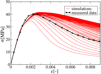
Following our experience [24], it is interesting to predict also the value of the constant $c_{20}$. Therefore, new 70 simulations (60 for training and 10 for testing purposes, respectively) were performed with fixed values of $E$, $\nu$ and $k_{1}$ parameters. The resulting bundle of curves can be compared to measured data, see Figure 3b. The same discretization was respected. The topology and inputs for the neural network are presented in Table 4 and errors in ANN’s predictions are listed in Table 5.

Parameter	Topology	Inputs
$c_{20}$	$4+2+1$	$\sigma_{[0.003]},\sigma_{[0.004]},\sigma_{[0.006]},\sigma_{[0.008]}$

Table 4: Topology of neural network for constant $c_{20}$ identification.

Parameter	Training data		Testing data
	Maximal error	Average error	Maximal error	Average error
$c_{20}$	11.18	6.02	11.27	6.15

Table 5: Errors in ANN’s prediction of constant $c_{20}$ relative to the size of admisible domain given for the $c_{20}$ parameter in [%].

Neural networks were applied on measured data and following value was obtained: $c_{20}=0.72785$.

Figure 5: Comparison of measured data and predicted simulations for uniaxial compression test.

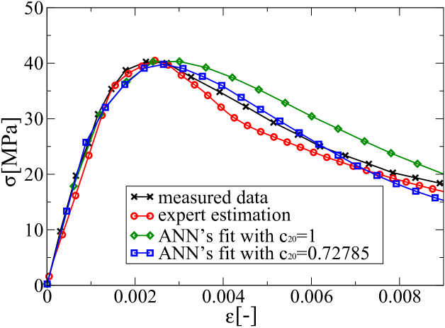
The final comparison of measured data and predicted simulations is shown in Figure 5. To show some more objective comparison of presented simulations, the error between measured data and simulated curves can be summarized over discrete points corresponding to measured data, i.e.

$$E=\|\mbox{\boldmath$\sigma$}-\tilde{\mbox{\boldmath$\sigma$}}\|,$$ (1)

where $\mbox{\boldmath$\sigma$}=[\dots,\sigma_{i},\dots]$ corresponds to stresses measured in discrete points $i$ and $\tilde{\mbox{\boldmath$\sigma$}}=[\dots,\tilde{\sigma}_{i},\dots]$ are corresponding simulated values. Values of the error defined by Equation 1 are shown in Table 6.

Prediction	Error $E$
expert estimation [7]	8.30
ANN + $c_{20}=1$	12.88
ANN + $c_{20}=0.72785$	6.97

Table 6: Comparison of errors of predicted simulations.

4.2 HYDROSTATIC COMPRESSION TEST

The next independent test used for the identification problem is the hydrostatic compression test, where a concrete cylinder is subjected to an increasing uniform pressure. Experimental data come again from [7]. These data were obtained by authors Green and Swanson [10]. The stress-strain diagram represents the relation of hydrostatic pressure $\sigma$ and axial deformation $\varepsilon$. The results from simulation performed for microplane model parameters obtained by expert estimation are there also available in comparison with measured data.

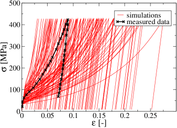
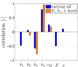
We suppose that values of Young’s modulus, Poisson’s ratio and $k_{1}$ parameter can be reliably obtained from uniaxial compression test. If not, they cannot be easily estimated from hydrostatic compression as their sensitivity to this experiment is relatively low, see Figure  6b, where maximal achieved sensitivities are plotted for the case of varying all the microplane parameters and the case with their fixed (known) values. Nevertheless, their low influence on the material behavior is still high enough to deteriorate the sensitivity of $k_{3}$ and $k_{4}$ parameters which may be then harder to identify.

Since the values of Young’s modulus, Poisson’s ratio and $k_{1}$ parameter are nevertheless not available for the concrete observed here, their values are taken directly from [7]. Then, the goal is to identify values of parameters $k_{3}$ and $k_{4}$; parameter $k_{2}$ attains almost zero sensitivity here. The bundle of resulting stress-strain diagrams for training and testing sets can be compared with measured data in Figure 6a.

(a)	(b)

Figure 6: Hydrostatic compression test: (a) comparison of measured data and results of 70 simulations; (b) maximal sensitivities.

Parameter	ANN’s layout	Input values
$k_{4}$	3 + 2 + 1	$k_{3}$, $\epsilon_{\mathrm{peak}}$, $\epsilon_{[85.5],\mathrm{unload}}$

Table 7: Neural network architecture for $k_{4}$ parameter identification; $\epsilon_{[85.5],u}$ is the deformation corresponding to hydrostatic stress $\hat{\sigma}=85.5$ MPa in the unloading phase.

During the verification process, we have not been able to properly identify the $k_{3}$ and $k_{4}$ parameters. Since all other parameters have very small or zero correlation, we suppose that the nonlinearity in the parameter $k_{3}$ identification is caused by $k_{4}$ parameter and vice-versa. In other words, these difficulties can be caused by some level of correlation between the parameters $k_{3}$ and $k_{4}$. Therefore, to eliminate unknown correlation between the parameters $k_{3}$ and $k_{4}$, their values are used also as inputs into ANNs.

All the inputs and architecture of the ANN for predicting $k_{4}$ parameter are given in Table 7. The inputs to an ANN for prediction of $k_{3}$ parameter were chosen in two different ways in order to show an impact of their particular selection to prediction of the post-elastic loading part of the stress-strain diagram. Two neural networks were trained with the deformation value (i) in the middle of loading phase with stress $\hat{\sigma}=214$ MPa and (ii) in its thirds: $\hat{\sigma}=137$ MPa and $\hat{\sigma}=308$ MPa leading to topologies given in Table 8. Note that the second ANN puts more emphasis on the post-elastic part of the diagram than the first one.

	Topology	Inputs
ANN1	$4+2+1$	$k_{4}$, $\epsilon_{\mathrm{peak}}$, $\epsilon_{\mathrm{yield}}$, $\epsilon_{[214],\mathrm{load}}$
ANN2	$5+2+1$	$k_{4}$, $\epsilon_{\mathrm{peak}}$, $\epsilon_{\mathrm{yield}}$, $\epsilon_{[137],\mathrm{load}}$, $\epsilon_{[308],\mathrm{load}}$

Table 8: Description of two neural networks trained to predict $k_{3}$ parameter

Parameter	Training data		Testing data
	Average error	Maximal error	Average error	Maximal error
$k_{3}$	1.40	2.59	1.71	3.07
$k_{4}$	1.51	2.52	1.21	2.13

Table 9: Error in ANN’s predictions relative to the size of admisible domain given for the parameters in [%].

Errors in predictions for training and testing data are listed in Table 9. For the sake of brevity only the errors corresponding to the first ANN trained for $k_{3}$ parameter are presented. The errors of the second network were negligibly higher.

Figure 7: Relations of $k_{3}$ and $k_{4}$ parameters for measured data: red continuous curve represents ANN trained to predict $k_{4}$ parameter, black dash-and-dot curve corresponds to ANN trained to predict $k_{3}$ parameter with four inputs (ANN₁) and blue dash curve to five inputs (ANN₂).

Two neural networks obtained to predict the $k_{3}$ and $k_{4}$ parameters with inputs taken from measured data represent system of two non-linear equations, which can be solved numerically. Solutions of particular equations are shown in Figure 7. The intersection of presented curves (i.e. solution of both equations) defines the predicted values of $k_{3}$ and $k_{4}$ parameters corresponding to measured data, in this case $k_{3}=12.34$, $k_{4}=98.19$ and $k_{3}=11.20$, $k_{4}=91.85$ for first and second neural networks, respectively.

In both cases, the predicted values differ from values given by authors in [7], where $k_{3}=9$ and $k_{4}=82$. The comparison of measured data with simulated diagrams obtained for parameters given in [7] and for two couples of parameters predicted by neural networks is depicted in Figure 8.

Figure 8: Comparison of measured data and simulated diagrams of hydrostatic compression test for predicted parameters.

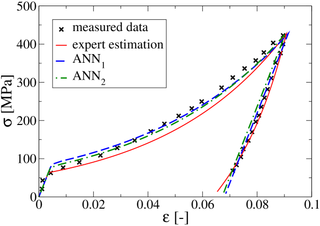
It is not so easy to judge which predicted simulation really better corresponds to measured data. A simulation presented in [7] relatively well fits the measured data at the end of elasticity and at the end of loading. Nevertheless, there is a significant error in the middle of the loading part of the diagram. One can notice that the accuracy of ANN’s prediction correspond to the choice of ANN’s inputs. The simulation for the ANN₁ prediction fits relatively well the measured data in the middle of the loading diagram, while the simulation for the ANN₂ prediction fits the data better near to the end of elasticity and to the end of the loading. To show more objective comparison of presented simulations, the error between measured data and simulated curves can be evaluated similarly to Eq. (1) just in terms of deformation instead of stresses. The values of the resulting error are presented in Table 10.

Prediction	Error $E$
expert estimation [7]	0.0257
ANN1	0.0163
ANN2	0.0161

Table 10: Comparison of errors of predicted simulations.

From the comparison presented in Table 10 it is clearly visible that simulations performed for parameters predicted by both neural networks fit the measured data better than the simulation done for parameters obtained by expert estimation presented in [7]. Moreover, it is also visible that simulations predicted by neural networks are somehow handicapped. Particular implementation of the microplane model M4 in the OOFEM software is slightly simplified and thus it does not properly describe material behavior during the hydrostatic unloading. While the full microplane model accounts for nonlinear response within the unloading phase, the version in OOFEM software assumes here only linear behavior. This model imperfection of course induce higher error in the experimental data fits obtained for ANNs’ predictions and one can expect that for the full microplane model simulations ANNs will achieve even better results.

4.3 TRIAXIAL COMPRESSION TEST

The last experiment, used for the purpose of parameter identification, is a triaxial compression test. To this end, a specimen is subjected to the hydrostatic pressure $\sigma_{H}$. After the peak value of $\sigma_{H}$ is reached, the axial stress is proportionally increased. The “excess” axial strain $\varepsilon=\varepsilon_{T}-\varepsilon_{H}$, where $\varepsilon_{T}$ and $\varepsilon_{H}$ denote the total and hydrostatic axial strain, is measured as a function of the overall stress $\sigma$. Similarly to the hydrostatic compression test, also for triaxial compression test we use measured data from [7]. These data were obtained by Balmer [4]. Again, the presented measured data are accompanied by the simulation performed by the authors of [7] for parameter values established by the expert estimation. The triaxial compression test is supposed to be the last experiment needed to identify parameters, which cannot be identified by uniaxial or hydrostatic compression tests, i.e. $k_{2}$ parameter. Therefore, Young’s modulus, Poisson’s ratio, $k_{1}$, $k_{3}$ and $k_{4}$ parameters are supposed to be known and their values are taken directly from [7].

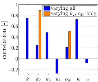
If the triaxial test is the only one available, the other parameters can be also identified. However, they will be predicted probably with higher errors, since the sensitivity analysis for varying all the parameters shows the highest value of sensitivity to Young’s modulus only $0.723$ (see Figure  9b), while its value in uniaxial test achieves $0.996$. Nevertheless, despite the uniaxial or hydrostatic tests, the triaxial test is the only one sensitive to all the microplane parameters.

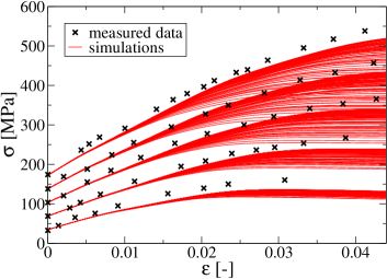
Five different measurements for the triaxial compression test are available in [7] corresponding to five different levels of a hydrostatic pressure $\sigma_{H}$ applied to specimens ($\sigma_{H}\in\{34.5,68.9,103.4,137.9,172.4\}$ MPa). The bundle of 70 resulting stress-strain diagrams can be compared with measured data in Figure 9a.

(a)	(b)

Figure 9: Triaxial compression test: (a) comparison of measured data and results of 70 simulations; (b) maximal sensitivities.

In Figure 9a it is clearly visible that measured data are remote from all simulated curves. This can be caused by wrong limits for $k_{2}$ parameter, i.e. $k_{2}\in(100;1000)$, however an increase of the upper bound by a factor of two did not bring substantial shift towards experimental data [16]. The discrepancy can be also caused by other parameters. Nevertheless, the goal of this Section is not to identify these parameters from triaxial compression test and therefore, we will test the ability of a neural network to cope with this problem.

Parameter	ANN’s layout	Input values
$k_{2}$	3 + 2 + 1	$\sigma_{\mathrm{peak}}$, $\sigma_{[0.0128]}$, $\sigma_{[0.0308]}$

Table 11: Neural network architecture for $k_{2}$ parameter identification.

A neural network with an architecture presented in Table 11 was trained on simulated data and then applied to predict a value of $k_{2}$ parameter for measured data. Note that only data from the lowest loading level were used. Errors of ANN’s predictions on training and testing samples are written in Table 12.

Parameter	Training data		Testing data
	Average error	Maximal error	Average error	Maximal error
$k_{2}$	2.63	5.82	2.37	6.23

Table 12: Error in ANN’s predictions relative to the size of admisible domain given for the $k_{2}$ parameter in [%].

The prediction of the neural network for measured data is $k_{2}=1193$, while $k_{2}=1000$ is suggested in [7]. It is not surprising that the neural network needs to extrapolate and its prediction exceeds the limit given for $k_{2}$ parameter. Although layered neural networks are known to be good in approximations, they are week in extrapolation. Moreover, there is a question, whether it is possible to find appropriate value of $k_{2}$ parameter to fit measured data, since it is probable that a more important error is hidden elsewhere. Finally, Figure 10 shows the comparison of measured data, a simulation given in [7] and a simulation for the parameter value predicted by the neural network.

Figure 10: Comparison of measured data and simulated diagrams of triaxial compression test for predicted parameters.

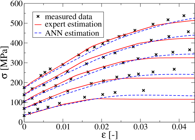
Similarly to previous sections, errors between measured data and simulated curves can be calculated. Resulting values for all five experiments corresponding to different levels of hydrostatic pressure $\sigma_{H}$ are shown in Table 13.

$\sigma_{H}$ [MPa]	expert estimation [7]	ANN’s predictions
34.5	64	43
68.9	87	60
103.4	73	45
137.9	70	39
172.4	43	60

Table 13: Comparison of errors of predicted simulations for triaxial compression test.

Errors in Table 13 are very similar for both simulations. It is possible to conclude that even for remote input data the neural network is able to predict a reasonable value of $k_{2}$ parameter and the resulting simulation seems to be better than the one obtained by the expert estimation. Moreover, the data from only one test with an arbitrary level of hydrostatic pressure $\sigma_{H}$ are sufficient for the parameter estimation and prediction of material behavior in case of different level of hydrostatic pressure.

5 Conclusions

In this contribution, an example of the engineering problem, which is difficult to be solved by traditional procedures, was solved using soft computing methods. Particularly, cascade neural networks were used to estimate required microplane material model parameters in a sequential way. As the training procedure, the evolutionary-based method GRADE extended by CERAF strategy was used. A number of needed simulations is reduced by the application of the Latin Hypercube Sampling method accompanied by the optimization by Simulated Annealing. The global sensitivity analysis shows not only the influence of individual parameters but also approximately predicts the errors produced by neural networks.

Parameter Test ANN’s topology ANN’s inputs $E$ Uniaxial compression $3+2+1$ $\sigma_{[0.0005]}$, $\sigma_{[0.001]}$, $\sigma_{[0.0015]}$ $k_{1}$ Uniaxial compression $5+3+1$ $\sigma_{[0.0025]}$, $\sigma_{[0.009]}$, $\sigma_{\mathrm{peak}}$, $\epsilon_{\mathrm{peak}}$, prediction of $E$ $k_{2}$ Triaxial loading $3+2+1$ $\sigma_{\mathrm{peak}}$, $\sigma_{[0.0128]}$, $\sigma_{[0.0308]}$ $k_{3}$ Hydrostatic loading $5+2+1$ $k_{4}$, $\epsilon_{\mathrm{yield}}$, $\epsilon_{[137],\mathrm{load}}$, $\epsilon_{[308],\mathrm{load}}$, $\epsilon_{\mathrm{peak}}$ $k_{4}$ Hydrostatic loading $3+2+1$ $k_{3}$, $\epsilon_{\mathrm{peak}}$, $\epsilon_{[85.5],\mathrm{unload}}$ $c_{20}$ Uniaxial compression $4+2+1$ $\sigma_{[0.003]}$, $\sigma_{[0.004]}$, $\sigma_{[0.006]}$, $\sigma_{[0.008]}$

Table 14: Final status of M4 identification project

Results, see Table 14, confirm the claims made by authors [7] of the microplane M4 model on individual parameters fitting. However, the validation of the complete process cannot be done, since the experimental data for all three loading tests performed on one concrete are not available and probably still do not exist. Therefore, the validation demonstrated in this paper is done only for particular identification steps.

Figure 11: Time required to access particular point on the uniaxial load-deflection curve.

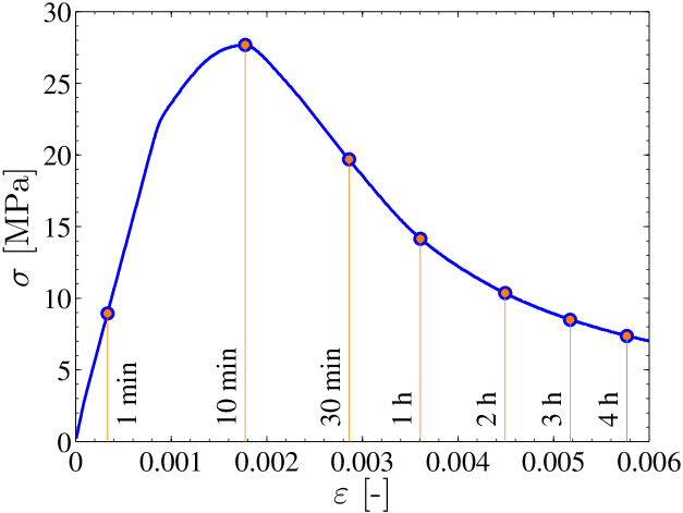
The rather severe disadvantage of the microplane model, and also of the proposed methodology, is an extreme demand of computational time. However, especially the uniaxial test dramatically depends on how far the computation will be processed. If we inspect Figure 11, every $0.001$ move on the softening branch costs in average one hour on a single processor PC with the Pentium IV 3400 MHz processor and 3 GB RAM. However there is a problem that individual compositions lead to big differences in times. This is illustrated in Figure 12, where the scatter of times is shown in a form of histograms. The averages are 8 minutes, 19 minutes and one hour for hydrostatic, triaxial and uniaxial compression tests, respectively. However note, that in cases that the material is very soft and the load-deflection curve is long, some computations longer than 6 hours can appear.

Figure 12: Histogram of times needed to run individual tests. The uniaxial test is measured at $\epsilon=0.004$ to fit the figure.

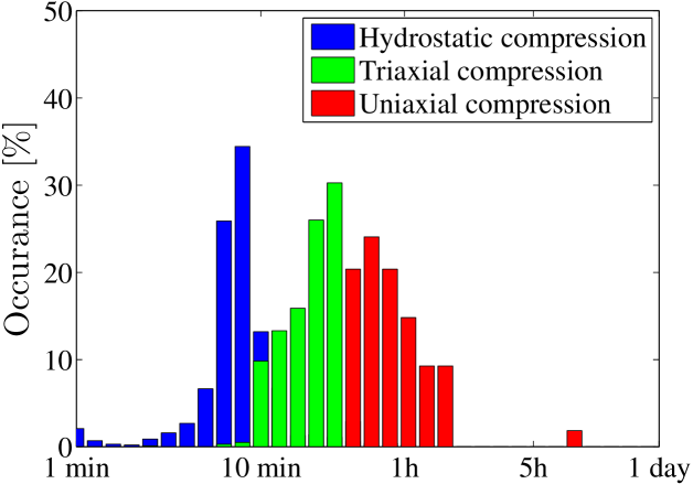
Because the identification procedure consists of developing cascade neural networks, all but one level inverse models should be recalculated for any new measured data. Fortunately, the most time consuming simulations of the uniaxial compression test are necessary for training of the first three neural networks predicting Young’s modulus, Poisson’s ratio and $k_{1}$ and can be used repeatedly for any new measurement. Then the proposed methodology still needs to compute 30 uniaxial tests to properly identify $c_{20}$ parameter and a set of 30 hydrostatic and triaxial tests to fit $k_{3}$, $k_{4}$ and $k_{2}$.

Acknowledgement

Financial support for this work was provided by the project CEZ MSM 6840770003 of Ministry of Education, Youth and Sports of the Czech Republic and by the projects P105/11/P370 and P105/12/1146 of the Czech Science Foundation. The financial support is gratefully acknowledged.

References

- [1]
- [2] H. Adeli. Neural networks in civil engineering: 1989–2000. Computer-Aided Civil and Infrastructure Engineering, 16(2):126–142, 2001.
- [3] I. Babuska and J. T. Oden. Verification and validation in computational engineering and science: basic concepts. Comput. Methods Appl. Mech. Engrg., 193:4057–4066, 2004.
- [4] G. G. Balmer. Shearing strength of concrete under high triaxial stress computation of mohr s envelope as a curve. Technical Report No. SP-23, U.S. Department of the Interior and Bureau of Reclamation, Denver, 1949.
- [5] Z.P. Bažant, F.C. Caner, I. Carol, M.D. Adley, and S.A. Akers. Microplane model M4 for concrete. I: Formulation with work-conjugate deviatoric stress. Journal of Engineering Mechanics-ASCE, 126(9):944–953, 2000.
- [6] Ch. M. Bishop. Neural Networks for Pattern Recognition. Oxford University Press, 1995.
- [7] F.C. Caner and Z.P. Bažant. Microplane model M4 for concrete. II: Algorithm and calibration. Journal of Engineering Mechanics-ASCE, 126(9):954–961, 2000.
- [8] G.V. Cybenko. Approximation by superpositions of a sigmoidal function. Mathematics of Control, Signals and Systems, 2(4):303–314, 1989.
- [9] J. Drchal, A. Kučerová, and J. Němeček. Optimizing synaptic weights of neural networks. In B.H.V. Topping and Z. Bittnar, editors, Proceedings of the Third International Conference on Engineering Computational Technology, Civil-Comp Press, Stirlingshire, UK, Paper 86, 2002. doi:10.4203/ccp.76.86.
- [10] S. J. Green and S. R. Swanson. Static constitutive relations for concrete. Technical Report AFWL-TR-72-2, Air Force Weapons Lab., Kirtland Air Force Base, Albuquerque, N.M., 1973.
- [11] Peter Holmes. Correlation: From picture to formula. Teaching Statistics, 23(3), Autumn 2001.
- [12] M. E. Jirásek and Z. P. Bažant. Inelastic Analysis of Structures. John Wiley & Sons, 2001.
- [13] P. Kordík. GAME – hybrid self-organizing modeling system based on GMDH. In Hybrid Self-Organizing Modeling Systems, volume 211 of Studies in Computational Intelligence, pages 233–280. Springer Berlin / Heidelberg, 2009.
- [14] A. Kučerová and T. Mareš. Self-adaptive Artificial Neural Network in Numerical Models Calibration. In Artificial Neural Networks - ICANN 2010, volume 1, pages 347–350, Berlin, 2010. Springer-Verlag.
-
[15]
A. Kučerová.
Homepage of CERAF.
http://klobouk.fsv.cvut.cz/~anicka/ceraf/ceraf.html. - [16] A. Kučerová. Identification of nonlinear mechanical model parameters based on softcomputing methods. PhD thesis, Ecole Normale Supérieure de Cachan, Laboratoire de Mécanique et Technologie, 2007.
- [17] A. Kučerová, D. Brancherie, A. Ibrahimbegović, J. Zeman, and Z. Bittnar. Novel anisotropic continuum-discrete damage model capable of representing localized failure of massive structures. part ii: identification from tests under heterogeneous stress field. Engineering Computations, 26(1/2):128–144, 2009.
[18]
A. Kučerová and M. Lepš.
Homepage of GRADE.
http://klobouk.fsv.cvut.cz/~anicka/grade/grade.html. - [19] A. Kučerová, M. Lepš, and J. Zeman. Back analysis of microplane model parameters using soft computing methods. Computer Assisted Mechanics and Engineering Sciences, 14(2):219–242, 2007. (Special issue of The International Symposium on Neural Networks and Soft Computing (NNSC-2005)).
- [20] M. Lepš. Load-balancing of Master-Slave Evolutionary Algorithm for Parameters Identification. In Proceedings of the First International Conference on Parallel, Distributed and Grid Computing for Engineering, Stirling, 2009. Civil-Comp Press Ltd.
- [21] R. Mahnken. Encyclopedia of Computational Mechanics Part 2. Solids and Structures, chapter Identification of Material Parameters for Constitutive Equations. John Wiley & Sons, Ltd., 2004.
- [22] R. Mahnken and E. Stein. Parameter identification for viscoplastic models based on analytical derivatives of a least-squares functional and stability investigations. International Journal of Plasticity, 12(4):451–479, 1996.
- [23] D. C. Montgomery. Design and Analysis of Experiments. John Wiley and Sons, 6 edition, 2005.
- [24] J. Němeček. Modeling of Compressive Softening of Concrete. PhD thesis, Czech Technical University in Prague, Praha, 2000.
- [25] D. Novák and D. Lehký. ANN inverse analysis based on stochastic small-sample training set simulation. Engineering Applications of Artificial Intelligence, 19:731–740, 2006.
- [26] D. Novák, M. Vořechovský, and R. Rusina. Small-sample probabilistic assessment - software FREET. In Proceedings of 9 International Conference on Applications of Statistic and Prabability in Civil Engineering - ICASP 9, pages 91–96, San Francisco, USA, 2003. Millpress, Rotterdam.
- [27] J. Němeček, B. Patzák, D. Rypl, and Z. Bittnar. Microplane models: Computational aspects and proposed parallel algorithm. Computers & Structures, 80(27–30):2099–2108, 2002.
- [28] B. Patzák. OOFEM home page. http://www.oofem.org, 2012.
- [29] B. Patzák and Z. Bittnar. Design of object oriented finite element code. Advances in Engineering Software, 32(10-11):759–767, 2001.
- [30] B. Pichler, R. Lackner, and H.A. Mang. Back analysis of model parameters in geotechnical engineering by means of soft computing. International Journal for Numerical Methods in Engineering, 57(14):1943–1978, 2003.
- [31] J. G. M. van Mier. Strain-softening of concrete under multiaxial loading conditions. PhD thesis, De Technische Hogeschool Eindhoven, The Netherlands, 1984.
- [32] J. Červenka, Z.P. Bažant, and M. Wierer. Equivalent localization element for crack band approach to mesh-sensitivity in microplane model. International Journal for Numerical Methods in Engineering, 62(5):700–726, 2005.
- [33] Z Waszczyszyn and L. Ziemiański. Parameter identification of materials and structures, chapter Neural networks in the identification analysis of structural mechanics problems, pages 265–340. Springer Wien / NewYork, 2005.
- [34] X. Yao. Evolving artificial neural networks. Proceedings of the IEEE, 87(9):1423–1447, 1999.