Discontinuous Galerkin method for fractional convection-diffusion equations

Abstract

We propose a discontinuous Galerkin method for convection-subdiffusion equations with a fractional operator of order $\alpha(1<\alpha<2)$ defined through the fractional Laplacian. The fractional operator of order $\alpha$ is expressed as a composite of first order derivatives and fractional integrals of order $2-\alpha$, and the fractional convection-diffusion problem is expressed as a system of low order differential/integral equations and a local discontinuous Galerkin method scheme is derived for the equations. We prove stability and optimal order of convergence ${\cal O}(h^{k+1})$ for subdiffusion, and an order of convergence of ${\cal O}(h^{k+\frac{1}{2}})$ is established for the general fractional convection-diffusion problem. The analysis is confirmed by numerical examples.

1 Introduction

In this paper we consider the following convection diffusion equation

$$\left\{\begin{array}[]{ll}\frac{\partial u(x,t)}{\partial t}+\frac{\partial}{\partial x}f(u)=\varepsilon\left(-(-\Delta)^{\alpha/2}\right)u(x,t),\quad x\in\mathbb{R},t\in(0,T],\\ u(x,0)=u_{0}(x),\quad x\in\mathbb{R}\end{array}\right.$$ (3)

where $f$ is assumed to be Lipschitz continuous and the subdiffusion is defined through the fractional Laplacian $-(-\Delta)^{\alpha/2}(\alpha\in(0,2])$, which can be defined using Fourier analysis as[22, 33, 37, 24],

$$-\widehat{(-\Delta)^{\alpha/2}}u(\xi)=(2\pi)^{\alpha}|\xi|^{\alpha}\hat{u}(\xi)$$ (4)

Equivalently, the fractional Laplacian can also be defined by a singular integral[3, 33],

$$-(-\Delta)^{\frac{\alpha}{2}}u(x)=c_{\alpha}\int_{|z|>0}\frac{u(x+z)-u(x)}{|z|^{1+\alpha}}dz$$ (5)

Equation (3), also known as a fractional conservation law, can be viewed as a generalization of the classical convection diffusion equation. During the last decade, it has arisen as a suitable model in many application areas, such as geomorphology[25, 26, 2], overdriven detonations in gases[14, 1], signal processing[5], anomalous diffusion in semiconductor growth [36] etc. With the special choice of $f(u)=u^{2}/2$, it is recognized as a fractional version of the viscous Burgers’ equation. Fractional conservation laws, especially Burgers’ equation, has been studied by many authors from a theoretical perspective, mainly involving questions of well-posedness and regularity of the solutions[27, 3, 31, 30, 20]. In the case of $\alpha<1$, the solution is in general not smooth and shocks may appear even with smooth initial datum. Similar to the classical scalar conservation laws, an appropriate entropy formulation is needed to guarantee well-posedness[3, 4]. For the case $\alpha>1$, the existence and uniqueness of a regular solution has been proved in [3, 30]. In this case, the nonlocal term serves as subdiffusion term, and smooth out discontinuities from initial datum.

Numerical studies of partial differential equations with nonlocal operator have attracted a lot of interest in recent years. Liu, Deng et al. have worked on numerical methods for fractional diffusion problems with fractional Laplacian operators or Riesz fractional derivatives [17, 40, 29, 19]. Briani, Cont, Matache, et al. have considered numerical methods for financial model with fractional Laplacian operators[9, 16, 32]. However, for conservation laws with fractional Laplacian operators, the development of accurate and robust numerical methods remains limited. Droniou is the first to analyze a general class of difference methods for fractional conservation laws[21]. Azeras proposed a class of finite difference schemes for solving a fractional antidiffusive equation[6]. Bouharguane proposed a splitting methods for the nonlocal Fowler equation in [8]. For the case $\alpha<1$, Cifani et al. [12, 13] applied the discontinuous Galerkin method to the fractional conservation law and degenerate convection diffusion equations and developed some error estimation. Unfortunately, their numerical results failed to confirm their analysis.

The discontinuous Galerkin method is a well established method for classical conservation laws [28]. However, for equations containing higher order spatial derivatives, discontinuous Galerkin methods cannot be directly applied[15, 39]. A careless application of the discontinuous Galerkin method to a problem with high order derivatives could yield an inconsistent method. The idea of local discontinuous Galerkin methods [15] for time dependent partial differential equations with higher derivatives is to rewrite the equation into a first order system and then apply the discontinuous Galerkin method to the system. A key ingredient for the success of this methods is the correct design of interface numerical fluxes. These fluxes must be designed to guarantee stability and local solvability of all the auxiliary variables introduced to approximate the derivatives of the solution.

In this paper, we will consider fractional convection diffusion equations with a fractional Laplacian operator of order $\alpha(1<\alpha<2)$. Especially for $1<\alpha<2$, it is conceptionally similar to a fractional derivative with an order between 1 and 2. To obtain a consistent and high accuracy method for this problem, we shall rewrite the fractional operator as a composite of first order derivatives and a fractional integral, and convert the fractional convection diffusion equation into a system of low order equations. This allows us to apply the local discontinuous Galerkin method.

This paper is organized as follows. In Section 2, we introduce some basic definitions and state a few central lemmas. In Section 3, we will derive the discontinuous Galerkin formulation for the fractional convection-diffusion law. In section 4, we develop stability and convergence analysis for fractional diffusion and convection-diffusion equations. In Section 5 some numerical examples are carried out to support our analysis. Conclusions are offered in Section 6.

2 Background and definitions

Apart from the definitions of the fractional Laplacian based on the Fourier and integral form above, it can also be defined using ideas of fractional calculus[22, 33, 40], as

$$-(-\Delta)^{\alpha/2}u(x)=\frac{\partial^{\alpha}}{\partial|x|^{\alpha}}u(x)=-\frac{{{}_{-\infty}D_{x}^{\alpha}}u(x)+{{}_{x}D_{\infty}^{\alpha}}u(x)}{2\cos\left(\frac{\alpha\pi}{2}\right)}$$ (6)

where $\prescript{}{-\infty}{D}_{x}^{\alpha}$ and $\prescript{}{x}{D}_{\infty}^{\alpha}$ refer to the left and right Riemann-Liouville fractional derivatives, respectively, of $\alpha$’th order. This definition is also known as a Riesz derivative. In this paper, we will based our developments and analysis mainly on this definition and will, in preparation, introduce a few definitions and properties of fractional integral/derivative to set the stage.

The left and right fractional integrals of order $\alpha$ are defined as

$${{}_{-\infty}I_{x}^{\alpha}}u(x)=\frac{1}{\Gamma(\alpha)}\int_{-\infty}^{x}(x-t)^{\alpha-1}u(t)dt$$ (7)

$${{}_{x}I_{\infty}^{\alpha}}u(x)=\frac{1}{\Gamma(\alpha)}\int^{\infty}_{x}(t-x)^{\alpha-1}u(t)dt$$ (8)

This allows for the definition of the left and right Riemann-Liouville fractional derivative of order $\alpha$ $(n-1<\alpha<n)$ as,

$${{}_{-\infty}D_{x}^{\alpha}}u(x)=\frac{1}{\Gamma(n-\alpha)}\left(\frac{d}{dx}\right)^{n}\int_{-\infty}^{x}(x-t)^{n-1-\alpha}u(t)dt=D^{n}({{}_{-\infty}I_{x}^{n-\alpha}}u(x))$$ (9)

$${{}_{x}D_{\infty}^{\alpha}}u(x)=\frac{1}{\Gamma(n-\alpha)}\left(-\frac{d}{dx}\right)^{n}\int^{\infty}_{x}(t-x)^{n-1-\alpha}u(t)dt=(-D)^{n}({{}_{x}I_{\infty}^{n-\alpha}}u(x))$$ (10)

Mirroring this, Caputo’s left and right fractional derivatives of order $\alpha$ $(n-1<\alpha<n)$ are defined as

$${\prescript{C}{-\infty}{D}_{x}^{\alpha}}u(x)=\frac{1}{\Gamma(n-\alpha)}\int_{-\infty}^{x}(x-t)^{n-1-\alpha}\left(\frac{d}{dt}\right)^{n}u(t)dt={{}_{-\infty}I_{x}^{n-\alpha}}(D^{n}u(x))$$ (11)

$${\prescript{C}{x}{D}_{\infty}^{\alpha}}u(x)=\frac{1}{\Gamma(n-\alpha)}\int^{\infty}_{x}(t-x)^{n-1-\alpha}\left(-\frac{d}{dt}\right)^{n}u(t)dt={{}_{x}I_{\infty}^{n-\alpha}}\left((-D)^{n}u(x)\right)$$ (12)

The two definitions, the Riemann-Liouville fractional derivative and Caputo’s fractional derivatives, are naturally related and they are equivalent provided all derivatives less than order $n$ of $u(x)$ disappear when $x\to\pm\infty$.

Fractional integrals and derivatives satisfy the following properties,

Lemma 1.

(Linearity[34]).

$$\prescript{}{-\infty}{I}_{x}^{\alpha}(\lambda f(x)+\mu g(x))=\lambda\prescript{}{-\infty}{I}_{x}^{\alpha}f(x)+\mu\prescript{}{-\infty}{I}_{x}^{\alpha}g(x)$$ (13)

$$\prescript{}{-\infty}{D}_{x}^{\alpha}(\lambda f(x)+\mu g(x))=\lambda\prescript{}{-\infty}{D}_{x}^{\alpha}f(x)+\mu\prescript{}{-\infty}{D}_{x}^{\alpha}g(x)$$ (14)

Lemma 2.

(Semigroup property[34]). For $\alpha,\beta>0$

$$\prescript{}{-\infty}{I}_{x}^{\alpha+\beta}f(x)=\prescript{}{-\infty}{I}_{x}^{\alpha}\left(\prescript{}{-\infty}{I}_{x}^{\beta}f(x)\right)=\prescript{}{-\infty}{I}_{x}^{\beta}\left(\prescript{}{-\infty}{I}_{x}^{\alpha}f(x)\right)$$ (15)

Lemma 3.

[34] Suppose $u^{(j)}(x)=0$,when $x\to\pm\infty,\forall\,0\leqslant j\leqslant n$ ( $n-1<\alpha<n$), then

$$\prescript{}{-\infty}{D^{\alpha}_{x}}u(x)=D^{n}\left(\prescript{}{-\infty}{I^{n-\alpha}_{x}}u(x)\right)=\prescript{}{-\infty}{I^{n-\alpha}_{x}}\left(D^{n}u(x)\right)$$ (16)

$$\prescript{}{x}{D^{\alpha}_{\infty}}u(x)=(-D)^{n}\left(\prescript{}{x}{I^{n-\alpha}_{\infty}}u(x)\right)=\prescript{}{x}{I^{n-\alpha}_{\infty}}\left((-D)^{n}u(x)\right)$$ (17)

From Lemma 3, we get, for $1<\alpha<2$ and a continuous function $u$ with $u^{(j)}(x)=0,x\to\pm\infty,0\leqslant j\leqslant 2$

$$-(-\Delta)^{\alpha/2}u(x) = -\frac{1}{2\cos(\alpha\pi/2)}\frac{d^{2}}{dx^{2}}\left({{}_{-\infty}I_{x}^{2-\alpha}}u(x)+{{}_{x}I_{\infty}^{2-\alpha}}u(x)\right)$$

$$= -\frac{1}{2\cos(\alpha\pi/2)}\frac{d}{dx}\left({{}_{-\infty}I_{x}^{2-\alpha}}\frac{du(x)}{dx}+{{}_{x}I_{\infty}^{2-\alpha}}\frac{du(x)}{dx}\right)$$

$$= -\frac{1}{2\cos(\alpha\pi/2)}\left({{}_{-\infty}I_{x}^{2-\alpha}}\frac{d^{2}u(x)}{dx^{2}}+{{}_{x}I_{\infty}^{2-\alpha}}\frac{d^{2}u(x)}{dx^{2}}\right)$$

For $0<s<1$, we define

$$\Delta_{-s/2}u(x)=-\frac{{{}_{-\infty}D_{x}^{-s}}u(x)+{{}_{x}D_{\infty}^{-s}}u(x)}{2\cos\left(\frac{(2-s)\pi}{2}\right)}=\frac{{{}_{-\infty}I_{x}^{s}}u(x)+{{}_{x}I_{\infty}^{s}}u(x)}{2\cos\left(\frac{s\pi}{2}\right)}$$

When $1<\alpha<2$, we have

$$-(-\Delta)^{\alpha/2}u(x)=\frac{d^{2}}{dx^{2}}\left(\Delta_{(\alpha-2)/2}u\right)=\Delta_{(\alpha-2)/2}\left(\frac{d^{2}u}{dx^{2}}\right)=\frac{d}{dx}\left(\Delta_{(\alpha-2)/2}\frac{du}{dx}\right)$$ (19)

To carry out the analysis, we introduce appropriate fractional spaces.

Definition 4.

(Left fractional space[23] ). We define the following seminorm

$$|u|_{J_{L}^{\alpha}(\mathbb{R})}=\|\prescript{}{-\infty}{D^{\alpha}_{x}}u\|_{L^{2}(\mathbb{R})}$$ (20)

and the norm

$$\|u\|_{J_{L}^{\alpha}(\mathbb{R})}=\left(|u|^{2}_{J_{L}^{\alpha}(\mathbb{R})}+\|u\|^{2}_{L^{2}(\mathbb{R})}\right)^{\frac{1}{2}}$$ (21)

and let $J_{L}^{\alpha}(\mathbb{R})$ denote the closure of $C_{0}^{\infty}(\mathbb{R})$ with respect to $\|\cdot\|_{J_{L}^{\alpha}}$.

Definition 5.

(Right fractional space[23] ). We define the following seminorm

$$|u|_{J_{R}^{\alpha}(\mathbb{R})}=\|\prescript{}{x}{D^{\alpha}_{\infty}}u\|_{L^{2}(\mathbb{R})}$$ (22)

and the norm

$$\|u\|_{J_{R}^{\alpha}(\mathbb{R})}=\left(|u|^{2}_{J_{R}^{\alpha}(\mathbb{R})}+\|u\|^{2}_{L^{2}(\mathbb{R})}\right)^{\frac{1}{2}}$$ (23)

and let $J_{R}^{\alpha}(\mathbb{R})$ denote the closure of $C_{0}^{\infty}(\mathbb{R})$ with respect to $\|\cdot\|_{J_{R}^{\alpha}}$.

Definition 6.

(Symmetric fractional space[23]) . We define the following seminorm

$$|u|_{J_{S}^{\alpha}(\mathbb{R})}=\left|\left(\prescript{}{-\infty}{D^{\alpha}_{x}}u,\prescript{}{x}{D^{\alpha}_{\infty}}u\right)_{L^{2}(\mathbb{R})}\right|^{\frac{1}{2}}$$ (24)

and the norm

$$\|u\|_{J_{S}^{\alpha}(\mathbb{R})}=\left(|u|^{2}_{J_{S}^{\alpha}(\mathbb{R})}+\|u\|^{2}_{L^{2}(\mathbb{R})}\right)^{\frac{1}{2}}$$ (25)

and let $J_{S}^{\alpha}(\mathbb{R})$ denote the closure of $C_{0}^{\infty}(\mathbb{R})$ with respect to $\|\cdot\|_{J_{S}^{\alpha}}$.

Using these definitions, we recover the following result,

Lemma 7.

(Adjoint property[35, 23])

$$\left({{}_{-\infty}I_{x}^{\alpha}}u,u\right)_{\mathbb{R}}=\left(u,{{}_{x}I_{\infty}^{\alpha}}u\right)_{\mathbb{R}}$$ (26)

Lemma 8.

[23]

$$\left({{}_{-\infty}I_{x}^{\alpha}}u,{{}_{x}I_{\infty}^{\alpha}}u\right)_{\mathbb{R}}=\cos(\alpha\pi)|u|^{2}_{J_{L}^{-\alpha}(\mathbb{R})}=\cos(\alpha\pi)|u|^{2}_{J^{-\alpha}_{R}({\mathbb{R}})}$$ (27)

From Lemma 7-8, we recover

Lemma 9.

For all $0<s<1$,

$$\left(\Delta_{-s}u,u\right)_{\mathbb{R}}=|u|^{2}_{J_{L}^{-s}(\mathbb{R})}=|u|^{2}_{J_{R}^{-s}(\mathbb{R})}$$ (28)

Generally, we consider the problem in a bounded domain instead of $\mathbb{R}$. Hence, we restrict the definition to the domain $\Omega=[a,b]$.

Definition 10.

Define the spaces $J^{\alpha}_{L,0}(\Omega),J^{\alpha}_{R,0}(\Omega),J^{\alpha}_{S,0}(\Omega))$ as the closures of $C_{0}^{\infty}(\Omega)$ under their respective norms.

For these fractional spaces, we have the following Theorem[18],

Theorem 11.

If $-\alpha_{2}<-\alpha_{1}<0$, then $J^{-\alpha_{1}}_{L,0}(\Omega)(\text{or}\,J^{-\alpha_{1}}_{R,0}(\Omega)\,\text{or}\,J^{-\alpha_{1}}_{S,0}(\Omega))$ is embedded into $J^{-\alpha_{2}}_{L,0}(\Omega)(\text{or}\,J^{-\alpha_{2}}_{R,0}(\Omega)\,\text{or}\,J^{-\alpha_{2}}_{S,0}(\Omega))$, and $L^{2}(\Omega)$ is embedded into both of them.

Lemma 12.

(Fractional Poincaré-Friedrichs)[23] For $u\in J^{\mu}_{L,0}(\Omega)$, we have

$$\|u\|_{L^{2}(\Omega)}\leqslant C|u|_{J^{\mu}_{L,0}},$$

and for $u\in J^{\mu}_{R,0}(\Omega)$, we have

$$\|u\|_{L^{2}(\Omega)}\leqslant C|u|_{J^{\mu}_{R,0}}.$$

From the definition of the left and right fractional integral, we obtain the following result,

Lemma 13.

Suppose the fractional integral is defined in $[0,b]$. Let $g(y)=f(b-x)$, then

$${{}_{x}I_{b}^{\alpha}}f(x)\overset{y=b-x}{=}{{}_{0}I_{y}^{\alpha}}g(y)$$ (29)

Lemma 14.

Suppose $u(x)$ is a smooth function $\in\Omega\subset\mathbb{R}$. $\Omega_{h}$ is a discretization of the domain with interval width $h$, $u_{h}(x)$ is an approximation of $u$ in $P_{h}^{k}$. $\forall$ i, $u_{h}(x)\in I_{i}$ is a polynomial of degree up to order $k$, and $(u,v)_{I_{i}}=(u_{h},v)_{I_{i}},\forall v\in P^{k}$. $k$ is the degree of the polynomial. Then for $-1<\alpha\leqslant 0$, we have

$$\|\Delta_{\alpha/2}u(x)-\Delta_{\alpha/2}u_{h}(x)\|_{L_{2}}\leqslant Ch^{k+1}$$

and for $0\leqslant n-1<\alpha\leqslant n,k\geqslant n$ we have

$$\|-(-\Delta)^{\frac{\alpha}{2}}u(x)+(-\Delta)^{\frac{\alpha}{2}}u_{h}(x)\|_{L_{2}}\leqslant Ch^{k+1-n}$$ (30)

where $C$ is a constant independent of $h$.

Proof.

Case $-1<\alpha\leqslant 0$,

First, we consider the approximation error for a fractional integral $\|\prescript{}{a}{I}^{-\alpha}_{x}u(x)-\prescript{}{a}{I}^{-\alpha}_{x}u_{h}(x)\|$.

First recall that $\|u(x)-u_{h}(x)\|_{2}=\mathcal{O}(h^{k+1})$ from classical approximation theory. Suppose $x\in\Omega_{h,i}$. We only need to consider $r^{i}=\prescript{}{a}{I}^{-\alpha}_{x}(\mathcal{O}(h^{k+1}))$.

$$r^{i} = \frac{1}{\Gamma(-\alpha)}\int_{a}^{x}(x-s)^{-\alpha-1}\mathcal{O}(h^{k+1})ds$$

$$\leqslant \frac{(b-a)^{-\alpha}\mathcal{O}(h^{k+1})}{\Gamma(1-\alpha)}$$

Recalling Lemma 13, the case $-1<\alpha\leqslant 0$ is proved.

The case $0\leqslant n-1<\alpha<n$, recall that $\|\frac{\partial^{n}u}{\partial x^{n}}-\frac{\partial^{n}u_{h}}{\partial x^{n}}\|\leqslant Ch^{k+1-n}$ and use the result for case $-1<\alpha\leqslant 0$, we obtain,

$$\|-(-\Delta)^{\frac{\alpha}{2}}u(x)+(-\Delta)^{\frac{\alpha}{2}}u_{h}(x)\|_{L_{2}}\leqslant Ch^{k+1-n}$$ (31)

This proves the Lemma. ∎

Lemma 15.

(Inverse properties[11]) Suppose $V_{h}$ is a finite element space spanned by polynomials up to degree $k$. For any $\omega_{h}\in V_{h}$, there exists a positive constant $C$ in dependent of $u_{h}$ and $h$, such that

$$\|\partial_{x}u_{h}\|\leqslant Ch^{-1}\|u_{h}\|,\quad\|u_{h}\|_{\Gamma_{h}}\leqslant Ch^{-\frac{1}{2}}\|u_{h}\|$$

3 LDG scheme for the fractional convection-diffusion equation

Let us consider the fractional convection-diffusion equation with $1<\alpha<2$. From (6) and Lemma 14, we know that a direct approximation of the fractional laplacian operator is of order $k+1-n$. To obtain a high order discontinuous Galerkin scheme for the fractional derivative, we rewrite the fractional derivative as a composite of first order derivatives and fractional integral and convert the equation to a low order system.

Following (19), we introduce two variables $p,q$, and set

$$q = \Delta_{(\alpha-2)/2}p$$

$$p = \sqrt{\varepsilon}\frac{\partial}{\partial x}u$$

Then, the fractional convection-diffusion problem can be rewritten as

$$\left\{\begin{array}[]{l}\frac{\partial u}{\partial t}+\frac{\partial}{\partial x}f(u)=\sqrt{\varepsilon}\frac{\partial}{\partial x}q\\ q=\Delta_{(\alpha-2)/2}p\\ p=\sqrt{\varepsilon}\frac{\partial}{\partial x}u\\ \end{array}\right.$$

Consider the equation in $\Omega=[a,b]$. Given a partition $a=x_{\frac{1}{2}}<x_{\frac{3}{2}}<\cdots<x_{K+\frac{1}{2}}=b$, we denote the mesh by $I_{j}=[x_{j-\frac{1}{2}},x_{j+\frac{1}{2}}]$, $\Delta x_{j}=x_{j+\frac{1}{2}}-x_{j-\frac{1}{2}}$.

We consider the solution in a polynomial space $V_{h}$, which is certainly embedded into the fractional space according to theorem 11. The piece-wise polynomial space $V_{h}$ on the mesh is defined as,

$$V_{h}=\{v:v\in P^{k}(I_{j}),x\in I_{j}\}$$

We seek an approximation $(u_{h},p_{h},q_{h})\in V_{h}$ to $(u,p,q)$ such that, for any $v,w,z\in V_{h}$, we have

$$\left\{\begin{array}[]{l}\left(\frac{\partial u_{h}(x,t)}{\partial t},v(x)\right)_{I_{i}}+\left(\frac{\partial}{\partial x}f(u_{h}),v(x)\right)_{I_{i}}=\sqrt{\varepsilon}\left(\frac{\partial q_{h}}{\partial x},v(x)\right)_{I_{i}}\\ \left(q_{h},w(x)\right)_{I_{i}}=\left(\Delta_{(\alpha-2)/2}p_{h},w(x)\right)_{I_{i}}\\ \left(p_{h},z(x)\right)_{I_{i}}=\sqrt{\varepsilon}\left(\frac{\partial u_{h}}{\partial x},z(x)\right)_{I_{i}}\\ \left(u_{h}(x,0),v(x)\right)_{I_{i}}=\left(u_{0}(x),v(x)\right)_{I_{i}}\end{array}\right.$$ (37)

To complete the LDG scheme, we introduce some notations and the numerical flux. Define

$$u^{\pm}(x_{j})=\lim_{x\to x^{\pm}_{j}}u(x),\;\;\bar{u}_{i}=\frac{u^{+}+u^{-}}{2},\quad\llbracket u\rrbracket=u^{+}-u^{-}$$

and the numerical flux as,

$$\hat{u}=h_{u}(u^{-},u^{+}),\quad\hat{q}=h_{q}(q^{-},q^{+}),\quad\hat{f_{h}}=\hat{f}(u_{h}^{-},u_{h}^{+})$$

For the high order derivative part, a good choice is the alternating direction flux[15, 39], defined as,

$$\hat{u}_{i+\frac{1}{2}}=u^{-}_{i+\frac{1}{2}},\quad\hat{q}_{i+\frac{1}{2}}=q^{+}_{i+\frac{1}{2}},0\leqslant i\leqslant K-1$$

or

$$\hat{u}_{i}=u^{+}_{i+\frac{1}{2}},\quad\hat{q}_{i}=q^{-}_{i+\frac{1}{2}},1\leqslant i\leqslant K$$

For the nonlinear part, $\hat{f}$, any monotone flux can be used [28].

Applying integration by parts to (37), and replacing the fluxes at the interfaces by the corresponding numerical fluxes, we obtain,

$$\left((u_{h})_{t},v\right)_{I_{i}}+\left(\hat{f_{h}}v-\sqrt{\varepsilon}\hat{q_{h}}v\right)|^{x^{-}_{i+\frac{1}{2}}}_{x^{+}_{i-\frac{1}{2}}}-\left(f(u_{h})-\sqrt{\varepsilon}q_{h},v_{x}\right)_{I_{i}} = 0$$ (38)

$$\left(q_{h},w(x)\right)_{I_{i}}-\left(\Delta_{(\alpha-2)/2}p_{h},w(x)\right)_{I_{i}} = 0$$ (39)

$$\left(p_{h},z(x)\right)_{I_{i}}-\sqrt{\varepsilon}\hat{u_{h}}z|^{x^{-}_{i+\frac{1}{2}}}_{x^{+}_{i-\frac{1}{2}}}+\sqrt{\varepsilon}\left(u_{h},z_{x}\right)_{I_{i}} = 0$$ (40)

$$\left(u_{h}(x,0),v(x)\right)_{I_{i}}-\left(u_{0}(x),v(x)\right)_{I_{i}} = 0$$ (41)

Remark 16.

Originally, the problem is defined in $\mathbb{R}$. However, for numerical purposes, we assume there existing a domain $\Omega=[a,b]\subset\mathbb{R}$ in which $u$ has compact support and restrict the problem to this domain $\Omega$. As a consequence, we impose homogeneous Dirichlet boundary conditions for all $u\in\mathbb{R}\backslash\Omega$. to recover

$$-(-\Delta)^{\alpha/2}u(x)=-\frac{{{}_{-\infty}D_{x}^{\alpha}}u(x)+{{}_{x}D_{\infty}^{\alpha}}u(x)}{2\cos\left(\frac{\alpha\pi}{2}\right)}=-\frac{{{}_{a}D_{x}^{\alpha}}u(x)+{{}_{x}D_{b}^{\alpha}}u(x)}{2\cos\left(\frac{\alpha\pi}{2}\right)}$$ (42)

For the flux at the boundary, we use the flux introduced in [10], defined as

$$\hat{u}_{K+\frac{1}{2}}=u(b,t),\quad\hat{q}_{K+\frac{1}{2}}=q^{-}_{K+\frac{1}{2}}+\frac{\beta}{h}\llbracket u_{K+\frac{1}{2}}\rrbracket$$

or

$$\hat{u}_{\frac{1}{2}}=u(a,t),\quad\hat{q}_{\frac{1}{2}}=q^{-}_{\frac{1}{2}}+\frac{\beta}{h}\llbracket u_{\frac{1}{2}}\rrbracket$$

where $\beta$ is a positive constant.

4 Stability and error estimates

In the following we shall discuss stability and accuracy of the proposed scheme, both for the fractional diffusion problem and the more general convection-diffusion problem.

4.1 Stability

In order to carry on analysis of the LDG scheme, we define

$$\mathscr{B}(u,p,q;v,w,z) = \int_{0}^{T}\sum_{i=1}^{K}\left(u_{t},v\right)_{I_{i}}dt+\int_{0}^{T}\sum_{i=1}^{K}\left(\hat{f}v-\sqrt{\varepsilon}\hat{q}v\right)|^{x^{-}_{i+\frac{1}{2}}}_{x^{+}_{i-\frac{1}{2}}}dt$$

$$-\int_{0}^{T}\sum_{i=1}^{K}\left(f(u)-\sqrt{\varepsilon}q,v_{x}\right)_{I_{i}}dt+\int_{0}^{T}\sum_{i=1}^{K}\left(q,w(x)\right)_{I_{i}}dt$$

$$-\int_{0}^{T}\sum_{i=1}^{K}\left(\Delta_{(\alpha-2)/2}p,w(x)\right)_{I_{i}}dt-\int_{0}^{T}\sum_{i=1}^{K}\sqrt{\varepsilon}\hat{u}z|^{x^{-}_{i+\frac{1}{2}}}_{x^{+}_{i-\frac{1}{2}}}dt$$

$$+\int_{0}^{T}\sum_{i=1}^{K}\left(p,z(x)\right)_{I_{i}}dt+\int_{0}^{T}\sum_{i=1}^{K}\sqrt{\varepsilon}\left(u,z_{x}\right)_{I_{i}}dt-\int_{0}^{T}\mathscr{L}(v,w,z)dt$$

where $\mathscr{L}$ contains the boundary term, defined as

$$\mathscr{L}(v,w,z)=\sqrt{\varepsilon}u(a,t)z^{+}_{\frac{1}{2}}-\frac{\sqrt{\varepsilon}\beta}{h}u(b,t)v^{-}_{K+\frac{1}{2}}dt+\sqrt{\varepsilon}u(b,t)z^{-}_{K+\frac{1}{2}}=0$$ (44)

If $(u,p,q)$ is a solution, then $\mathscr{B}(u,p,q;v,w,z)=0$ for any $(v,w,z)$. Considering the fluxes $\hat{u}_{i+\frac{1}{2}}=u^{-}_{i+\frac{1}{2}},\hat{q}_{i+\frac{1}{2}}=q^{+}_{i+\frac{1}{2}}$ and the flux at the boundaries we recover,

$$\mathscr{B}(u,p,q;v,w,z) = \int_{0}^{T}\sum_{i=1}^{K}\left(u_{t},v\right)_{I_{i}}dt-\int_{0}^{T}\sum_{i=1}^{K}\left(f(u),v_{x}\right)_{I_{i}}dt$$

$$+\int_{0}^{T}\sum_{i=1}^{K}\left(\sqrt{\varepsilon}q,v_{x}\right)_{I_{i}}dt+\int_{0}^{T}\sum_{i=1}^{K}\sqrt{\varepsilon}\left(u,z_{x}\right)_{I_{i}}dt+\int_{0}^{T}\sum_{i=1}^{K}\left(q,w(x)\right)_{I_{i}}dt$$

$$-\int_{0}^{T}\sum_{i=1}^{K}\left(\Delta_{(\alpha-2)/2}p,w(x)\right)_{I_{i}}dt+\int_{0}^{T}\sum_{i=1}^{K}\left(p,z(x)\right)_{I_{i}}dt$$

$$-\int_{0}^{T}\sum_{i=1}^{K-1}{\hat{f}_{i+\frac{1}{2}}}\llbracket v\rrbracket_{i+\frac{1}{2}}dt+\int_{0}^{T}\sum_{i=1}^{K-1}\sqrt{\varepsilon}{q^{+}_{i+\frac{1}{2}}}\llbracket v\rrbracket_{i+\frac{1}{2}}dt$$

$$+\int_{0}^{T}\sum_{i=1}^{K-1}\sqrt{\varepsilon}{u^{-}_{i+\frac{1}{2}}}\llbracket z\rrbracket_{i+\frac{1}{2}}dt-\int_{0}^{T}(\hat{f}_{\frac{1}{2}}v^{+}_{\frac{1}{2}}-\hat{f}_{K+\frac{1}{2}}v^{-}_{K+\frac{1}{2}})dt$$

$$+\int_{0}^{T}\sqrt{\varepsilon}(q^{+}_{\frac{1}{2}}v^{+}_{\frac{1}{2}}-q^{-}_{K+\frac{1}{2}}v^{-}_{K+\frac{1}{2}})dt+\int_{0}^{T}\frac{\sqrt{\varepsilon}\beta}{h}u^{-}_{K+\frac{1}{2}}v^{-}_{K+\frac{1}{2}}dt$$

Lemma 17.

Set $(v,w,z)=(u,-p,q)$ in (4.1), and define $\Phi(u)=\int^{u}f(u)du$. Then the following result holds,

$$\mathscr{B}(u,p,q;u,-p,q) = \|u(x,T)\|^{2}-\|u_{0}\|^{2}+\int_{0}^{T}(\Delta_{(\alpha-2)/2}p,p)dt+\int_{0}^{T}\frac{\sqrt{\varepsilon}\beta}{h}(u^{-}_{K+\frac{1}{2}})^{2}dt$$

$$+\int_{0}^{T}\Phi(u)_{\frac{1}{2}}-\Phi(u)_{K+\frac{1}{2}}-(\hat{f}u)_{\frac{1}{2}}+(\hat{f}u)_{K+\frac{1}{2}}dt$$

$$+\int_{0}^{T}\sum_{j=1}^{K-1}\left(\llbracket\Phi(u)\rrbracket_{j+\frac{1}{2}}-\hat{f}\llbracket u\rrbracket_{j+\frac{1}{2}}\right)dt$$

Proof.

Set $(v,w,z)=(u,-p,q)$ in (4.1), and consider the integration by parts formula $(q,u_{x})_{I_{i}}+(u,q_{x})_{I_{i}}=(uq)|_{x^{+}_{i-\frac{1}{2}}}^{x^{-}_{i+\frac{1}{2}}}$, to recover at an interface

$$\sum_{i=1}^{K}\left(\sqrt{\varepsilon}q,v_{x}\right)_{I_{i}}+\sum_{i=1}^{K}\left(\sqrt{\varepsilon}u,z_{x}\right)_{I_{i}}+\sum_{i=1}^{K-1}\sqrt{\varepsilon}{q^{+}_{i+\frac{1}{2}}}\llbracket v\rrbracket_{i+\frac{1}{2}}+\sum_{i=1}^{K-1}\sqrt{\varepsilon}{u^{-}_{i+\frac{1}{2}}}\llbracket z\rrbracket_{i+\frac{1}{2}}$$

$$= \sum_{i=1}^{K}\sqrt{\varepsilon}\left(uq\right)|^{x^{-}_{i+\frac{1}{2}}}_{x^{+}_{i-\frac{1}{2}}}+\sum_{i=1}^{K-1}\sqrt{\varepsilon}{q^{+}_{i+\frac{1}{2}}}\llbracket u\rrbracket_{i+\frac{1}{2}}+\sum_{i=1}^{K-1}\sqrt{\varepsilon}{u^{-}_{i+\frac{1}{2}}}\llbracket q\rrbracket_{i+\frac{1}{2}}$$

$$= -\sqrt{\varepsilon}q^{+}_{\frac{1}{2}}u^{+}_{\frac{1}{2}}+\sqrt{\varepsilon}q^{-}_{K+\frac{1}{2}}u^{-}_{K+\frac{1}{2}}$$

Then

$$\mathscr{B}(u,p,q;u,-p,q) = \int_{0}^{T}\sum_{i=1}^{K}\left(u_{t},u\right)_{I_{i}}dt-\int_{0}^{T}\sum_{i=1}^{K}\left(f(u),u_{x}\right)_{I_{i}}dt$$

$$-\int_{0}^{T}\sum_{i=1}^{K}\left(\Delta_{(\alpha-2)/2}p,p\right)_{I_{i}}dt-\int_{0}^{T}\sum_{i=1}^{K-1}{\hat{f}_{i+\frac{1}{2}}}\llbracket v\rrbracket_{i+\frac{1}{2}}dt$$

$$-\int_{0}^{T}(\hat{f}_{\frac{1}{2}}u^{+}_{\frac{1}{2}}-\hat{f}_{K+\frac{1}{2}}u^{-}_{K+\frac{1}{2}})dt+\int_{0}^{T}\frac{\sqrt{\varepsilon}\beta}{h}\left(u^{-}_{K+\frac{1}{2}}\right)^{2}dt$$

Define $\Phi(u)=\int^{u}f(u)du$, then

$$\sum_{i=1}^{K}\left(f(u),u_{x}\right)_{I_{i}}=\sum_{i=1}^{K}\Phi(x)|_{x^{+}_{i-\frac{1}{2}}}^{x^{-}_{i+\frac{1}{2}}}=-\sum_{i=1}^{K-1}\llbracket\Phi(u)\rrbracket_{i+\frac{1}{2}}-\Phi(u)_{\frac{1}{2}}+\Phi(u)_{K+\frac{1}{2}}$$ (47)

Combining (4.1) and (47) proves the Lemma. ∎

Theorem 18.

The semi-discrete scheme (38)-(41) is stable, and $\|u_{h}(x,T)\|\leqslant\|u_{0}(x)\|$ for any $T>0$.

Proof.

Using the properties of the monotone flux, $\hat{f}(u^{-},u^{+})$ is a non-decreasing function of its first argument, and a non-increasing function of its second argument. Hence, we have $\llbracket\Phi(u_{h})\rrbracket_{j+\frac{1}{2}}-\hat{f_{h}}\llbracket u_{h}\rrbracket_{j+\frac{1}{2}}>0,1\leqslant j\leqslant K-1$. By Galerkin orthogonality, $\mathscr{B}(u_{h},p_{h},q_{h};u_{h},-p_{h},q_{h})=0$, Lemma 17 yields

$$\|u(x,T)\|^{2}-\|u_{0}\|^{2}+\int_{0}^{T}(\Delta_{(\alpha-2)/2}p,p)dt+\int_{0}^{T}\frac{\sqrt{\varepsilon}\beta}{h}(u^{-}_{K+\frac{1}{2}})^{2}dt$$

$$+\int_{0}^{T}\Phi(u)_{\frac{1}{2}}-\Phi(u)_{K+\frac{1}{2}}-(\hat{f}u)_{\frac{1}{2}}+(\hat{f}u)_{K+\frac{1}{2}}dt\leqslant 0$$

Considering the boundary condition and Lemma 9, we obtain $\|u_{h}(x,T)\|\leqslant\|u_{0}(x)\|$, hence completing the proof. ∎

4.2 Error estimates

To estimate the error, we firstly consider fractional diffusion with the Laplacian operator, i.e., the case with $f=0$. For fractional diffusion, (38)-(41) reduce to

$$\left((u_{h})_{t},v\right)_{I_{i}}-(\sqrt{\varepsilon}\hat{q_{h}}v)|^{x^{-}_{i+\frac{1}{2}}}_{x^{+}_{i-\frac{1}{2}}}+\left(\sqrt{\varepsilon}q_{h},v_{x}\right)_{I_{i}} = 0$$ (48)

$$\left(q_{h},w(x)\right)_{I_{i}}-\left(\Delta_{(\alpha-2)/2}p_{h},w(x)\right)_{I_{i}} = 0$$ (49)

$$\left(p_{h},z(x)\right)_{I_{i}}-\sqrt{\varepsilon}\hat{u_{h}}z|^{x^{-}_{i+\frac{1}{2}}}_{x^{+}_{i-\frac{1}{2}}}+\sqrt{\varepsilon}\left(u_{h},z_{x}\right)_{I_{i}} = 0$$ (50)

$$\left(u_{h}(x,0),v(x)\right)_{I_{i}}-\left(u_{0}(x),v(x)\right)_{I_{i}} = 0$$ (51)

Correspondingly, we have the compact form of the scheme as

$$\mathscr{B}(u,p,q;v,w,z) = \int_{0}^{T}\sum_{i=1}^{K}\left(u_{t},v\right)_{I_{i}}dt+\int_{0}^{T}\sum_{i=1}^{K}\sqrt{\varepsilon}\left(q,v_{x}\right)_{I_{i}}dt+\int_{0}^{T}\sum_{i=1}^{K}\sqrt{\varepsilon}\left(u,z_{x}\right)_{I_{i}}dt$$ (52)

$$+\int_{0}^{T}\sum_{i=1}^{K}\left(q,w(x)\right)_{I_{i}}dt-\int_{0}^{T}\sum_{i=1}^{K}\left(\Delta_{(\alpha-2)/2}p,w(x)\right)_{I_{i}}dt+\int_{0}^{T}\sum_{i=1}^{K}\left(p,z(x)\right)_{I_{i}}dt$$

$$+\int_{0}^{T}\sum_{i=1}^{K-1}\sqrt{\varepsilon}{q^{+}_{i+\frac{1}{2}}}\llbracket v\rrbracket_{i+\frac{1}{2}}dt+\int_{0}^{T}\sum_{i=1}^{K-1}\sqrt{\varepsilon}{u^{-}_{i+\frac{1}{2}}}\llbracket z\rrbracket_{i+\frac{1}{2}}dt$$

$$+\int_{0}^{T}\sqrt{\varepsilon}q^{+}_{\frac{1}{2}}v^{+}_{\frac{1}{2}}dt+\int_{0}^{T}\frac{\sqrt{\varepsilon}\beta}{h}u^{-}_{K+\frac{1}{2}}v^{-}_{K+\frac{1}{2}}dt-\int_{0}^{T}\sqrt{\varepsilon}q^{-}_{K+\frac{1}{2}}v^{-}_{K+\frac{1}{2}}dt$$

To prepare for the main result, we first obtain a few central Lemmas. We define special projections, $\mathscr{P}^{\pm}$ and $\mathscr{Q}$ into $V_{h}$, which satisfy, for each $j$,

$$\int_{I_{j}}(\mathscr{P}^{\pm}u(x)-u(x))v(x)dx=0\quad\forall v\in P^{k-1}\quad\text{and}\quad\mathscr{P}^{\pm}u_{j+\frac{1}{2}}=u(x^{\pm}_{j+\frac{1}{2}})$$ (53)

$$\int_{I_{j}}(\mathscr{Q}u(x)-u(x))v(x)dx=0\quad\forall v\in P^{k}$$ (54)

Denote $e_{u}=u-u_{h},e_{p}=p-p_{h},e_{q}=q-q_{h}$, then

$$\mathscr{P}^{-}e_{u}=\mathscr{P}^{-}u-u_{h},\mathscr{P}^{+}e_{q}=\mathscr{P}^{+}q-q_{h},\mathscr{Q}e_{p}=\mathscr{Q}p-p_{h}$$

For any $(v,w,z)\in H^{1}(\Omega,\mathcal{T})\times L^{2}(\Omega,\mathcal{T})\times L^{2}(\Omega,\mathcal{T})$ ,

$$\mathscr{B}(u,p,q;v,w,z)=\mathscr{L}(v,w,z)$$ (55)

Hence, $\mathscr{B}(e_{u},e_{p},e_{q};v,w,z)=0$ and we recover

$$\mathscr{B}(\mathscr{P}^{-}e_{u},\mathscr{Q}e_{p},\mathscr{P}^{+}e_{q};\mathscr{P}^{-}e_{u},-\mathscr{Q}e_{p},\mathscr{P}^{+}e_{q})$$

$$= \mathscr{B}(\mathscr{P}^{-}e_{u}-e_{u},\mathscr{Q}e_{p}-e_{p},\mathscr{P}^{+}e_{q}-e_{q};\mathscr{P}^{-}e_{u},-\mathscr{Q}e_{p},\mathscr{P}^{+}e_{q})$$

$$= \mathscr{B}(\mathscr{P}^{-}u-u,\mathscr{Q}p-p,\mathscr{P}^{+}q-q;\mathscr{P}^{-}e_{u},-\mathscr{Q}e_{p},\mathscr{P}^{+}e_{q})$$

Substitute $(\mathscr{P}^{-}u-u,\mathscr{Q}p-p,\mathscr{P}^{+}q-q;\mathscr{P}^{-}e_{u},-\mathscr{Q}e_{p},\mathscr{P}^{+}e_{q})$ into (52), to recover the following Lemma,

Lemma 19.

For the bilinear form, (52), we have

$$\mathscr{B}(\mathscr{P}^{-}u-u,\mathscr{Q}p-p,\mathscr{P}^{+}q-q;\mathscr{P}^{-}e_{u},-\mathscr{Q}e_{p},\mathscr{P}^{+}e_{q})$$

$$\leqslant \int_{0}^{T}\sum_{i=1}^{K}\left((\mathscr{P}^{-}u)_{t}-u_{t},\mathscr{P}^{-}e_{u}\right)_{I_{i}}dt+C_{T,a,b}h^{2k+2}+\frac{1}{C_{T,a,b}}\int_{0}^{T}\sum_{i=1}^{K}\|\mathscr{Q}e_{p}\|_{I_{i}}^{2}dt$$

$$+\int_{0}^{T}\frac{\sqrt{\varepsilon}\beta}{h}|(\mathscr{P}^{-}e_{u})^{-}_{K+\frac{1}{2}}|^{2}dt$$

where $C_{T,a,b}$is independent of $h$, but may dependent of $T$ and $\Omega$.

Proof.

From (52) we have

$$\mathscr{B}(\mathscr{P}^{-}u-u,\mathscr{Q}p-p,\mathscr{P}^{+}q-q;\mathscr{P}^{-}e_{u},-\mathscr{Q}e_{p},\mathscr{P}^{+}e_{q})$$

$$= \int_{0}^{T}\sum_{i=1}^{K}\left((\mathscr{P}^{-}u)_{t}-u_{t},\mathscr{P}^{-}e_{u}\right)_{I_{i}}dt+\int_{0}^{T}\sum_{i=1}^{K}\sqrt{\varepsilon}\left(\mathscr{P}^{+}q-q,(\mathscr{P}^{-}e_{u})_{x}\right)_{I_{i}}dt$$

$$+\int_{0}^{T}\sum_{i=1}^{K}\sqrt{\varepsilon}\left(\mathscr{P}^{-}u-u,(\mathscr{P}^{+}e_{q})_{x}\right)_{I_{i}}dt-\int_{0}^{T}\sum_{i=1}^{K}\left(\mathscr{P}^{+}q-q,\mathscr{Q}e_{p}\right)_{I_{i}}dt$$

$$+\int_{0}^{T}\sum_{i=1}^{K}\left(\Delta_{(\alpha-2)/2}(\mathscr{Q}p-p),\mathscr{Q}e_{p}\right)_{I_{i}}dt+\int_{0}^{T}\sum_{i=1}^{K}\left(\mathscr{Q}p-p,\mathscr{P}^{+}e_{q}\right)_{I_{i}}dt$$

$$+\int_{0}^{T}\sum_{i=1}^{K-1}\sqrt{\varepsilon}(\mathscr{P}^{+}q-q)^{+}_{i+\frac{1}{2}}\llbracket\mathscr{P}^{-}e_{u}\rrbracket_{i+\frac{1}{2}}+\int_{0}^{T}\sum_{i=1}^{K-1}\sqrt{\varepsilon}(\mathscr{P}^{-}u-u)^{-}_{i+\frac{1}{2}}\llbracket\mathscr{P}^{+}e_{q}\rrbracket_{i+\frac{1}{2}}$$

$$+\int_{0}^{T}\sqrt{\varepsilon}(\mathscr{P}^{+}q-q)^{+}_{\frac{1}{2}}\llbracket\mathscr{P}^{-}e_{u}^{+}\rrbracket_{\frac{1}{2}}dt+\int_{0}^{T}\frac{\sqrt{\varepsilon}\beta}{h}(\mathscr{P}^{-}u-u)^{-}_{K+\frac{1}{2}}\llbracket\mathscr{P}^{-}e_{u}^{-}\rrbracket_{K+\frac{1}{2}}dt$$

$$-\int_{0}^{T}\sqrt{\varepsilon}(\mathscr{P}^{+}q-q)^{-}_{K+\frac{1}{2}}\llbracket\mathscr{P}^{-}e_{u}^{-}\rrbracket_{K+\frac{1}{2}}dt$$

Since $(\mathscr{P}^{-}e_{u})_{x}\in P^{k-1},(\mathscr{P}^{+}e_{q})_{x}\in P^{k-1},(\mathscr{Q}e_{p})_{x}\in P^{k-1},\mathscr{Q}e_{p}\in P^{k}$, by the properties of the projection $\mathscr{P}^{\pm},\mathscr{Q}$, we recover,

$$\left(\mathscr{P}^{+}q-q,(\mathscr{P}^{-}e_{u})_{x}\right)_{I_{i}}=0,\quad\left(\mathscr{P}^{-}u-u,(\mathscr{P}^{+}e_{q})_{x}\right)_{I_{i}}=0$$

$$\left(\mathscr{Q}p-p,\mathscr{P}^{+}e_{q}\right)_{I_{i}}=0,\quad\left(\mathscr{Q}p-p,(\mathscr{P}^{+}e_{q})_{x}\right)_{I_{i}}=0$$

$$(\mathscr{P}^{-}u-u)_{i+\frac{1}{2}}=0,\quad(\mathscr{P}^{+}q-q)_{i+\frac{1}{2}}=0.$$

We obtain,

$$\mathscr{B}(\mathscr{P}^{-}u-u,\mathscr{Q}p-p,\mathscr{P}^{+}q-q;\mathscr{P}^{-}e_{u},-\mathscr{Q}e_{p},\mathscr{P}^{+}e_{q})$$

$$= \int_{0}^{T}\sum_{i=1}^{K}\left((\mathscr{P}^{-}u)_{t}-u_{t},\mathscr{P}^{-}e_{u}\right)_{I_{i}}dt-\int_{0}^{T}\sqrt{\varepsilon}(\mathscr{P}^{+}q-q^{-})_{K+\frac{1}{2}}(\mathscr{P}^{-}e_{u})^{-}_{K+\frac{1}{2}}dt$$

$$+\int_{0}^{T}\sum_{i=1}^{K}\left(\Delta_{(\alpha-2)/2}(\mathscr{Q}p-p)-(\mathscr{P}^{+}q-q),\mathscr{Q}e_{p}\right)_{I_{i}}dt$$

Recalling the projection property and Lemma 14, we obtain $\|\Delta_{(\alpha-2)/2}(\mathscr{Q}p-p)-(\mathscr{P}^{+}q-q)\|\leqslant Ch^{k+1}$. Combining this with Young’s inequality and (15), we obtain

$$\mathscr{B}(\mathscr{P}^{-}u-u,\mathscr{Q}p-p,\mathscr{P}^{+}q-q;\mathscr{P}^{-}e_{u},-\mathscr{Q}e_{p},\mathscr{P}^{+}e_{q})$$

$$\leqslant \int_{0}^{T}\sum_{i=1}^{K}\left((\mathscr{P}^{-}u)_{t}-u_{t},\mathscr{P}^{-}e_{u}\right)_{I_{i}}dt+C_{T,a,b}h^{2k+2}+\frac{1}{C_{T,a,b}}\int_{0}^{T}\sum_{i=1}^{K}\|\mathscr{Q}e_{p}\|_{I_{i}}^{2}dt$$

$$+\int_{0}^{T}\frac{\sqrt{\varepsilon}\beta}{h}|(\mathscr{P}^{-}e_{u})_{K+\frac{1}{2}}|^{2}dt$$

This proves the lemma. ∎

Lemma 20.

[10] Suppose that for all $t>0$ we have

$$\chi^{2}(t)+R(t)\leqslant A(t)+2\int_{0}^{t}B(s)\chi(s)ds,$$

where $R,A,B$ are nonnegative functions. Then, for any $T>0$,

$$\sqrt{\chi^{2}(T)+R(t)}\leqslant\sup_{0\leqslant t\leqslant T}A^{1/2}(t)+\int_{0}^{T}B(t)dt$$

Theorem 21.

Let $u$ be the a sufficiently smooth exact solution to (3) in $\Omega\subset\mathbb{R}$ with $f(u)=0$. Let $u_{h}$ be the numerical solution of the semi-discrete LDG scheme (38)-(41), then for small enough $h$, we have the following error estimates

$$\|u-u_{h}\|\leqslant Ch^{k+1}$$

where $C$ is a constant independent of $h$.

Proof.

From Lemma 17 and the initial error $\|\mathscr{P}^{-}e_{u}(0)\|=0$, we have

$$B(\mathscr{P}^{-}e_{u},\mathscr{Q}e_{p},\mathscr{P}^{+}e_{q};\mathscr{P}^{-}e_{u},-\mathscr{Q}e_{p},\mathscr{P}^{+}e_{q})$$

$$= \frac{1}{2}\|\mathscr{P}^{-}e_{u}(T)\|^{2}+\int_{0}^{T}\left(\Delta_{(\alpha-2)/2}\mathscr{Q}e_{p},\mathscr{Q}e_{p}\right)_{I_{i}}dt+\int_{0}^{T}\frac{\sqrt{\varepsilon}\beta}{h}|\mathscr{P}^{-}e_{u}|^{2}_{K+\frac{1}{2}}dt$$

Combining this with Lemma 19 and (4.2), we have

$$\frac{1}{2}\|\mathscr{P}^{-}e_{u}(T)\|^{2}+\int_{0}^{T}\left(\Delta_{(\alpha-2)/2}\mathscr{Q}e_{p},\mathscr{Q}e_{p}\right)dt$$

$$\leqslant \int_{0}^{T}\left((\mathscr{P}^{-}u)_{t}-u_{t},\mathscr{P}^{-}e_{u}\right)dt+C_{T,a,b}h^{2k+2}+\frac{1}{C_{T,a,b}}\int_{0}^{T}\|\mathscr{Q}e_{p}\|^{2}dt$$

Recalling the fractional Poincaré-Friedrichs Lemma 12, we get

$$\frac{1}{2}\|\mathscr{P}^{-}e_{u}(T)\|^{2}\leqslant\int_{0}^{T}\left((\mathscr{P}^{-}u)_{t}-u_{t},\mathscr{P}^{-}e_{u}\right)dt+C_{T,a,b}h^{2k+2}$$

Using Lemma 20 and the error associated with the projection error, proves the theorem. ∎

For the more general fractional convection-diffusion problem, we introduce a few results and then give the error estimate.

Lemma 22.

[41] For any piecewise smooth function $\omega\in L^{2}(\Omega)$, on each cell boundary point we define

$$\kappa(\hat{f};\omega)\equiv\kappa(\hat{f};\omega^{-},\omega^{+})\triangleq\left\{\begin{array}[]{l l}[\omega]^{-1}(f(\bar{\omega})-\hat{f}(\omega))&\text{if}\quad[\omega]\neq 0,\\ \frac{1}{2}|f^{\prime}(\bar{\omega})|&\text{if}\quad[\omega]=0\end{array}\right.$$ (56)

where $\hat{f}(\omega)\equiv\hat{f}(\omega^{-},\omega^{+})$ is a monotone numerical flux consistent with the given flux $f$. Then $\kappa(\hat{f},\omega)$ is non-negative and bounded for any $(\omega^{-},\omega^{+})\in\mathbb{R}$. Moreover, we have

$$\frac{1}{2}|f^{\prime}(\bar{\omega})|\leqslant\kappa(\hat{f};\omega)+C_{*}|[\omega]|,$$ (57)

$$-\frac{1}{8}f^{\prime\prime}(\bar{\omega})[\omega]\leqslant\kappa(\hat{f};\omega)+C_{*}|[\omega]|^{2}.$$ (58)

Define

$$\sum_{j=1}^{K}\mathscr{H}_{j}(f;u,u_{h},v) = \sum_{j=1}^{K}\int_{I_{j}}(f(u)-f(u_{h}))v_{x}dx+\sum_{j=1}^{K}((f(u)-f(\bar{u_{h}}))[v])_{j+\frac{1}{2}}$$

$$+\sum_{j=1}^{K}((f(\bar{u_{h}})-\hat{f})[v])_{j+\frac{1}{2}}$$

Lemma 23.

[38] For $\mathscr{H}(f;u,u_{h},v)$ defined above, we have the following estimate

$$\sum_{j=1}^{K}\mathscr{H}_{j}(f;u,u_{h},v) \leqslant -\frac{1}{4}\kappa(\hat{f};u_{h})[v]^{2}+(C+C_{*}(\|v\|_{\infty}+h^{-1}\|e_{u}\|_{\infty}^{2}))\|v\|^{2}$$

$$+(C+C_{*}h^{-1}\|e_{u}\|_{\infty}^{2})h^{2k+1}$$

Combining Theorem 21 and Lemma 23, we recover the following error estimate

Theorem 24.

Let $u$ be the exact solution of (3), which is sufficiently smooth $\in\Omega\subset\mathbb{R}$ and assume $f\in C^{3}$. Let $u_{h}$ be the numerical solution of the semi-discrete LDG scheme (48)-(51) and denote the corresponding numerical error by $e_{u}=u-u_{h}$. $V_{h}$ is the space of piecewise polynomials of degree $k\geqslant 1$, then for small enough $h$, we have the following error estimates

$$\|u-u_{h}\|\leqslant Ch^{k+\frac{1}{2}}$$

Remark 25.

Although the order of convergence $k+\frac{1}{2}$ is obtained it can be improved if an upwind flux is chosen for $\hat{f}$. In this case, optimal order can be recovered. We shall demonstrate this in the numerical examples.

Remark 26.

For problems with mixed boundary conditions, another scheme may be more suitable for implementation. Suppose the problem has a Dirichlet boundary on the left end and a Neumann boundary at the right end. Let $p=\sqrt{\varepsilon}\frac{\partial u}{\partial x},q=\sqrt{\varepsilon}\frac{\partial p}{\partial x}$, then we have

$$\left\{\begin{array}[]{l}\frac{\partial u}{\partial t}+\frac{\partial}{\partial x}f(u)=\Delta_{(\alpha-2)/2}q\\ q=\sqrt{\varepsilon}\frac{\partial p}{\partial x}\\ p=\sqrt{\varepsilon}\frac{\partial u}{\partial x}\\ \end{array}\right.$$

Similarly, we have the following scheme,

$$\left((u_{h})_{t},v\right)_{I_{i}}+\hat{f_{h}}v|_{I_{i}}-\left(f(u_{h}),v_{x}\right)_{I_{i}}-\left(\Delta_{(\alpha-2)/2}q_{h},v(x)\right)_{I_{i}}=0$$ (60)

$$\left(q_{h},w(x)\right)_{I_{i}}-\sqrt{\varepsilon}\hat{p_{h}}w|_{I_{i}}+\sqrt{\varepsilon}\left(p_{h},w_{x}\right)_{I_{i}}=0$$ (61)

$$\left(p_{h},z(x)\right)_{I_{i}}-\sqrt{\varepsilon}\hat{u_{h}}z|_{I_{i}}+\sqrt{\varepsilon}\left(u_{h},z_{x}\right)_{I_{i}}=0$$ (62)

$$\left(u_{h}(x,0),v(x)\right)_{I_{i}}-\left(u_{0}(x),v(x)\right)_{I_{i}}=0$$ (63)

In this scheme, a mixed boundary condition is imposed naturally. However, the analysis is more complicated. While computational results indicate excellent behavior and optimal convergence, we shall not talk about the theoretical aspect of this scheme.

5 Numerical examples

In the following, we shall present a few results to numerically validate the analysis.

The discussion so far have focused on the treatment of the spatial dimension with a semi-discrete form as

$$\frac{d\mathbf{u}_{h}}{dt}=\mathcal{L}_{h}(\mathbf{u}_{h},t)$$ (64)

where $\mathbf{u}_{h}$ is the vector of unknowns. For the time discretization of the equations, we use a fourth order low storage explicit Runge-Kutta(LSERK) method[28] of the form,

$$\mathbf{p}^{0}=\mathbf{u}^{n},$$

$$i\in[1,\cdots,5]:\left\{\begin{array}[]{l}\mathbf{k}^{i}=a_{i}\mathbf{k}^{i-1}+\Delta t\mathcal{L}_{h}(\mathbf{p}^{i-1},t^{n}+c_{i}\Delta t)\\ \mathbf{p}^{(i)}=\mathbf{p}^{(i-1)}+b_{i}\mathbf{k}^{(i)},\end{array}\right.$$

$$\mathbf{u}_{h}^{n+1}=\mathbf{p}^{(5)}$$

where $a_{i},b_{i},c_{i}$ are coefficients of LSRK method given in [28]. For the explicit methods, proper timestep $\Delta t$ is needed. In our examples, numerically the condition $\Delta t\leqslant C\Delta x_{min}^{\alpha},(0<C<1)$ is necessary for stability.

Table 1: Error and order of convergence for solving the fractional Laplacian problem with $K$ elements and polynomial order $N$.

	$\alpha=1.1$
K	10	20		30		40
N	$\|e_{u}\|_{2}$	$\|e_{u}\|_{2}$	Order	$\|e_{u}\|_{2}$	Order	$\|e_{u}\|_{2}$	Order
	K= 10	K= 20	order	K= 30	order	K= 40	order
1	1.64e-06	3.98e-07	2.04	1.73e-07	2.05	9.60e-08	2.05
2	1.24e-07	1.69e-08	2.87	5.13e-09	2.94	2.18e-09	2.97
3	1.14e-08	7.23e-10	3.98	1.41e-10	4.03	4.44e-11	4.03
	$\alpha=1.3$
K	10	20		30		40
N	$\|e_{u}\|_{2}$	$\|e_{u}\|_{2}$	Order	$\|e_{u}\|_{2}$	Order	$\|e_{u}\|_{2}$	Order
	K= 10	K= 20	order	K= 30	order	K= 40	order
1	1.45e-06	3.46e-07	2.07	1.50e-07	2.06	8.33e-08	2.05
2	1.19e-07	1.55e-08	2.94	4.64e-09	2.98	1.96e-09	2.99
3	1.04e-08	6.48e-10	4.00	1.26e-10	4.03	3.97e-11	4.02
	$\alpha=1.5$
K	10	20		30		40
N	$\|e_{u}\|_{2}$	$\|e_{u}\|_{2}$	Order	$\|e_{u}\|_{2}$	Order	$\|e_{u}\|_{2}$	Order
1	1.35e-06	3.24e-07	2.06	1.42e-07	2.04	7.90e-08	2.03
2	1.22e-07	1.51e-08	3.01	4.51e-09	2.99	1.90e-09	2.99
3	1.04e-08	6.28e-10	4.05	1.22e-10	4.04	3.85e-11	4.02
	$\alpha=1.8$
K	10	20		30		40
N	$\|e_{u}\|_{2}$	$\|e_{u}\|_{2}$	Order	$\|e_{u}\|_{2}$	Order	$\|e_{u}\|_{2}$	Order
1	1.28e-06	3.11e-07	2.04	1.38e-07	2.01	7.74e-08	2.01
2	1.40e-07	1.51e-08	3.21	4.48e-09	3.00	1.89e-09	3.00
3	1.44e-08	6.72e-10	4.42	1.23e-10	4.19	3.83e-11	4.05

Example 1. As the first example, we consider the fractional diffusion equation with the fractional Laplacian,

$$\left\{\begin{array}[]{ll}\frac{\partial u(x,t)}{\partial t}=-(-\Delta)^{\alpha/2}u(x,t)+g(x,t),\quad in\quad[0,1]\times(0,0.5]\\ u(x,0)=u_{0}(x).\end{array}\right.$$ (68)

with the initial condition $u_{0}(x)=x^{6}(1-x)^{6}$, and the source term $g(x,t)=e^{-t}\left(-u_{0}(x)+(-\Delta)^{\frac{\alpha}{2}}u_{0}(x)\right)$
The exact solution is $u(x,t)=e^{-t}x^{6}(1-x)^{6}$.

The results are shown in Table 1 and we observe optimal ${\cal O}(h^{k+1})$ order of convergence across $1<\alpha<2$.

Table 2: Error and order of convergence for solving the fractional Burgers’ equation with $K$ elements and polynomial order $N$.

	$\alpha=1.01$
K	10	20		30		40
N	$\|e_{u}\|_{2}$	$\|e_{u}\|_{2}$	Order	$\|e_{u}\|_{2}$	Order	$\|e_{u}\|_{2}$	Order
	K= 10	K= 20	order	K= 30	order	K= 40	order
1	1.10e-03	2.81e-04	1.97	1.24e-04	2.03	6.90e-05	2.03
2	6.53e-05	1.00e-05	2.70	3.09e-06	2.90	1.33e-06	2.94
3	5.94e-06	4.00e-07	3.89	8.05e-08	3.96	2.58e-08	3.95
	$\alpha=1.5$
K	10	20		30		40
N	$\|e_{u}\|_{2}$	$\|e_{u}\|_{2}$	Order	$\|e_{u}\|_{2}$	Order	$\|e_{u}\|_{2}$	Order
1	8.89e-04	2.15e-04	2.05	9.45e-05	2.03	5.28e-05	2.02
2	6.71e-05	8.62e-06	2.96	2.57e-06	2.99	1.09e-06	2.99
3	4.91e-06	3.34e-07	3.88	6.80e-08	3.93	2.16e-08	3.99
	$\alpha=1.8$
K	10	20		30		40
N	$\|e_{u}\|_{2}$	$\|e_{u}\|_{2}$	Order	$\|e_{u}\|_{2}$	Order	$\|e_{u}\|_{2}$	Order
1	8.43e-04	2.09e-04	2.01	9.25e-05	2.01	5.20e-05	2.00
2	6.78e-05	8.59e-06	2.98	2.56e-06	2.99	1.08e-06	2.99
3	4.80e-06	3.32e-07	3.85	6.84e-08	3.90	2.20e-08	3.94

Example 2. We consider the fractional Burgers’ equation

$$\left\{\begin{array}[]{ll}\frac{\partial u(x,t)}{\partial t}+\frac{\partial}{\partial x}\left(\frac{u^{2}(x,t)}{2}\right)=\varepsilon(-(-\Delta)^{\alpha/2})u(x,t)+g(x,t),\quad in\quad[-2,2]\times(0,0.5]\\ u(x,0)=u_{0}(x).\end{array}\right.$$ (71)

with initial the condition

$$u_{0}(x)=\left\{\begin{array}[]{ll}(1-x^{2})^{4}/10&\ -1\leqslant x\leqslant 1\\ 0&\ \mbox{otherwise}\end{array}\right.$$

The source term $g(x,t)=e^{-t}\left(-u_{0}(x)+e^{-t}u_{0}(x)u^{\prime}_{0}(x)+\varepsilon(-\Delta)^{\frac{\alpha}{2}}u_{0}(x)\right),\varepsilon=1$ is derived to yield an exact solution as

$$u(x,t)=\left\{\begin{array}[]{ll}e^{-t}(1-x^{2})^{4}/10&\ -1\leqslant x\leqslant 1\\ 0&\ \mbox{otherwise}\end{array}\right.$$

The results are shown in Table 2 and we observe optimal ${\cal O}(h^{k+1})$ order of convergence across $1<\alpha<2$.

Example 3 Let us finally consider the fractional Burgers’ equation with a discontinuous initial condition,

$$u_{0}(x)=\left\{\begin{array}[]{ll}\frac{1}{2}&-1\leqslant x\leqslant 0\\ 0&\mbox{otherwise}\end{array}\right.$$

We consider the case in (71) with $\varepsilon=0.04$, $g(x,t)=0$.

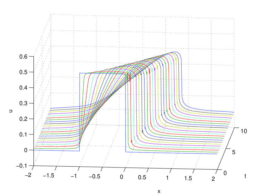
Fig. 1: Solution of the fractional Burgers’s equation with $\epsilon=0.04,\alpha=1.005$

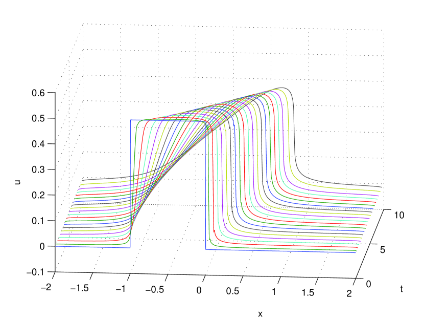
Fig. 2: Solution of the fractional Burgers’s equation with $\epsilon=0.04,\alpha=1.1$

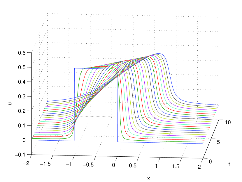
Fig. 3: Solution of the fractional Burgers’s equation with $\epsilon=0.04,\alpha=1.5$

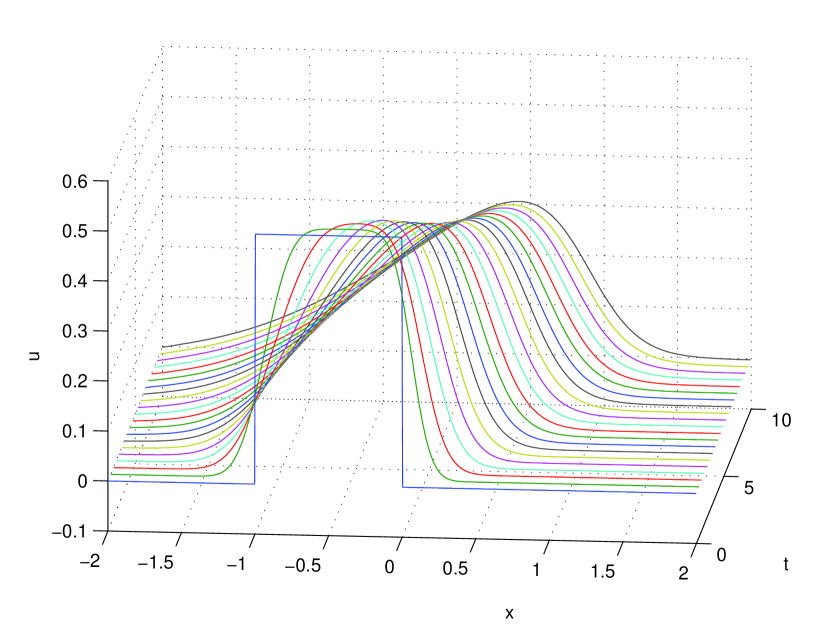
Fig. 4: Solution of the fractional Burgers’s equation with $\epsilon=0.04,\alpha=2.0$

The increasing dissipative effect of increasing $\alpha$ is clear from the sequence of figures, Fig. (2)-(4), with the latter case of $\alpha=2$ being the classic case.

6 Concluding remarks

We propose a discontinuous Galerkin method for convection-diffusion problems in which the a fractional diffusion is expressed through a fractional Laplacian. To obtain a high order accuracy, we rewrite the fractional Lapacian as a composite of first order derivatives and integrals and transform the problem to a low order system. We consider the equation in a domain $\Omega$ with homogeneous boundary conditions. A local discontinuous Galerkin method is proposed and stability and error estimations are derived, establishing optimal convergence. In the numerical examples, the analysis is confirmed for different values of $\alpha$.

References

- [1] M. Alfaro and J. Droniou, 2012, General Fractal Conservation Laws Arising from a Model of Detonations in Gases, Appl. Math. Res. Express, 2, pp. 127-151.
- [2] N. Alibaud, P. Azerad and D. Isèbe, 2007, A non-monotone conservation law for dune morphodynamics. arxiv.org/abs/0709.3360
- [3] N. Alibaud, J. Droniou and J. Vovelle, 2007, Occurrence and non-appearance of shocks in fractal Burgers equations, Journal of Hyperbolic Differential Equations, 4(3) pp. 479-499.
- [4] N. Alibaud, 2007, Entropy formulation for fractal conservation laws, Journal of Evolution Equations, 7, pp. 145-175.
- [5] P. Azerad, A. Bouharguane and J.-F. Crouzet, 2010, Simultaneous denoising and enhancement of signals by a fractal conservation law, preprint: http://arxiv4.library.cornell.edu/abs/1004.5193.
- [6] P. Azerad and A. Bouharguane, 2011, Finite difference approximations for a fractional diffusion/antidiffusion equation. http://arxiv.org/abs/1104.4861.
- [7] P. Biler, T. Funaki and W. Woyczinski, 1998, Fractal Burgers equations, Journal of Differential Equations, 148, pp. 9-46.
- [8] A. Bouharguane and R.Carles, 2011, Splitting methods for the nonlocal Fowler equation. Available from: http://arxiv.org/abs/1109.3275
- [9] M. Briani and R. Natalini, 2006, Asymptotic high-order schemes for integro-differential problems arising in markets with jumps, Commun. Math. Sci. 4, pp. 81-96.
- [10] P. Castillo, B. Cockburn , D. Schötzau and C. Schwab, 2003, Optimal a priori error estimates for the hp-version of the local discontinuous Galerkin method for convection-diffusion problems, Math. Comp. 71, pp. 455-478.
- [11] P. Ciarlet, 1975, The Finite Element Method for Elliptic Problem, North-Holland.
- [12] S. Cifani and E. R. Jakobsen, 2011, The discontinuous Galerkin method for fractal conservation laws, IMA Journal of Numerical Analysis 31, pp. 1090-1122.
- [13] S. Cifani, E. R. Jakobsen, and K. H. Karlsen, 2011, The discontinuous Galerkin method for fractional degenerate convection-diffusion equations. BIT 51(4), pp. 809-844.
- [14] P. Clavin, 2003, Instabilities and nonlinear patterns of overdriven detonations in gases. In Nonlinear PDE’s in Condensed Matter and Reactive Flows, NATO Science Series, 569(1), pp. 49-97.
- [15] B. Cockburn and C.-W. Shu, 1998, The local discontinuous Galerkin method for time-dependent convection-diffusion systems, SIAM Journal on Numerical Analysis 35(6), pp. 2440-2463.
- [16] R. Cont and V. Ekaterina, 2005, A finite difference scheme for option pricing in jump diffusion and exponential Lévy models, SIAM J. Numer. Anal., 43, pp. 1596-1626.
- [17] W. Deng, 2008, Finite Element Method for the Space and Time Fractional Fokker-Planck Equation, SIAM Journal on Numerical Analysis, 47(1), pp. 204-226.
- [18] W. Deng and J. S. Hesthaven, 2011, Discontinuous Galerkin method for fractional diffusion equation - (submitted).
- [19] H.-F. Ding and Y.-X. Zhang, 2012, New numerical methods for the Riesz space fractional partial differential equations, Computers and Mathematics with Applications 63, pp. 1135-1146.
- [20] H. Dong, D. Du and D. Li, 2009, Finite time singularities and global well-posedness for fractal Burgers equations, Indiana Univ. Math. J., 59, pp. 807-821.
- [21] J. Droniou, 2010, A numerical method for fractal conservation laws, Math. Comput. 79, pp. 95-124.
- [22] A. M. A. El-Sayed and M. Gaber, 2006, On the Finite Caputo and Finite Riesz Derivatives, Electronic Journal of Theoretical Physics, 3(12), pp. 81-95.
- [23] V.J. Ervin and J.P. Roop, 2010 Variational formulation for the stationary fractional advection dispersion equation, Numer. Methods Partial Differential Equations 22(3), pp. 558-576.
- [24] L C.F. Ferreira and E. J. Villamizar-Roa, 2011, Fractional Navier-Stokes equations and a H lder-type inequality in a sum of singular spaces, Nonlinear Analysis 74, pp. 5618-5630
- [25] A. C. Fowler, 2001. Dunes and drumlins, Geomorphological fluid mechanics, eds. A. Provenzale and N. Balmforth, Springer-Verlag, Berlin,211, pp. 430-454.
- [26] A. C. Fowler, 2002, Evolution equations for dunes and drumlins, Rev. R. Acad. de Cien, Serie A. Mat, 96(3), pp. 377-387.
- [27] A. Guesmia and N. Daili, 2010, About the existence and uniqueness of solution to fractional Burgers equation, Acta Universitatis Apulensis, 21, pp. 161-170.
- [28] J. S. Hesthaven and T. Warburton, 2008, Nodal Discontinuous Galerkin Methods: Algorithms, Analysis, and Applications, Springer-Verlag, New York, USA.
- [29] M.Ilic, F.Liu, I.Turner, and V.Anh, 2009, Numerical approximation of a fractional-in-space diffusion equation (II) - with nonhomogeneous boundary conditions, Fractional Calculus and applied analysis, 9(4), pp. 333-349.
- [30] A. Kiselev, F. Nazarov, and R. Shterenberg, 2008, Blow Up and Regularity for Fractal Burgers Equation, Dynamics of PDE, 5(3), pp. 211-240.
- [31] E. T. Kolkovska, 2005, Existence and regularity of solutions to a stochastic Burgers-type equation, Brazilian Journal of Probability and Statistics, 19, pp. 139-154.
- [32] A. Matache, C. Schwab and T. P. Wihler, 2005, Fast numerical solution of parabolic integrodifferential equations with applications in finance, SIAM J. Sci. Comput. 27, pp 369-393.
- [33] S. I. Muslih and O. P. Agrawal, 2010, Riesz Fractional Derivatives and Fractional Dimensional Space, Int. J. Theor. Phys. 49, pp. 270-275.
- [34] I. Podlubny, 1999, Fractional Differential Equations. Academic Press, New York.
- [35] S. G. Samko, A. A. Kilbas and O. I. Marichev, 1993, Fractional Integrals and Derivatives: Theory and Applications. Gordon and Breach, Amsterdam.
- [36] M.F. Shlesinger, G.M. Zaslavsky and U. Frisch, (Eds.), 1995, Lêvy Flights and related topics in physics. Lecture Notes in Physics 450, Springer-Verlag, Berlin.
- [37] J. Wu, 2005, Lower Bounds for an Integral Involving Fractional Laplacians and the Generalized Navier-Stokes Equations in Besov Spaces, Commun. Math. Phys. 263, pp. 803-831.
- [38] Y. Xu and C.-W. Shu, 2007, Error estimates of the semi-discrete local discontinuous Galerkin method for nonlinear convection-diffusion and KdV equations, Comput. Methods Appl. Mech. Engrg. 196, pp. 3805-3822.
- [39] J. Yan and C.-W. Shu, 2002, Local Discontinuous Galerkin Methods for Partial Differential Equations with Higher Order Derivatives, Journal of Scientific Computing, 17, pp. 27-47.
- [40] Q. Yang, F.Liu, and I.Turner, 2010, Numerical methods for fractional partial differential equations with Riesz space fractional derivatives, Appl.Math.Modelling 34, pp. 200-218.
- [41] Q. Zhang and C.-W. Shu, 2004, Error estimates to smooth solutions of Runge Kutta discontinuous Galerkin methods for scalar conservation laws, SIAM J. Numer. Anal. 42, pp. 641-666.