Characterisation of global flow and local fluctuations in 3D SPH simulations of protoplanetary discs

Abstract

A complete and detailed knowledge of the structure of the gaseous component in protoplanetary discs is essential to the study of dust evolution during the early phases of pre-planetesimal formation. The aim of this paper is to determine if three-dimensional accretion discs simulated by the Smoothed Particle Hydrodynamics (SPH) method can reproduce the observational data now available and the expected turbulent nature of protoplanetary discs. The investigation is carried out by setting up a suite of diagnostic tools specifically designed to characterise both the global flow and the fluctuations of the gaseous disc. The main result concerns the role of the artificial viscosity implementation in the SPH method: in addition to the already known ability of SPH artificial viscosity to mimic a physical-like viscosity under specific conditions, we show how the same artificial viscosity prescription behaves like an implicit turbulence model. In fact, we identify a threshold for the parameters in the standard artificial viscosity above which SPH disc models present a cascade in the power spectrum of velocity fluctuations, turbulent diffusion and a mass accretion rate of the same order of magnitude as measured in observations. Furthermore, the turbulence properties observed locally in SPH disc models are accompanied by meridional circulation in the global flow of the gas, proving that the two mechanisms can coexist.

1 Introduction

Protoplanetary discs (abbreviated PPD) are discs composed mainly of gas and dust in quasi-Keplerian rotation around young stars. They are believed to be the birth place of planets. The theory of planet formation is complex because several scales (from $\mu$m to hundreds of thousands of km), several forces (e.g. electrostatic, magnetic, gravitational, drag) and several processes (e.g. turbulence, chemical and thermodynamical transformations, instabilities) are involved. One of the more poorly understood stages is the evolution of $\mu$m-size dust grains into km-size objects, called planetesimals.

Among the several mechanisms the dust is subject to (e.g. radial drift and vertical settling), possible large scale motion and turbulence are expected to be of relevant importance. Large scale motion can lead dust to travel to very different locations in the disc. Turbulence can have two competing effects mediated by gas drag: stirring up and diffusing dust particles, impeding their agglomeration, or trapping them inside eddies, favoring their agglomeration (see e.g. Cuzzi et al., 1993; Carballido et al., 2008; Cuzzi et al., 2008).

Here we focus on the global flow and on the expected turbulent behaviour of only the gaseous component of PPD, which represents the medium in which dust evolves.

In the literature, two large classes of models of turbulent discs are widely used: continuous and discrete models. Continuous models of viscous discs are directly derived from the Navier-Stokes equations in presence of the gravitational potential of the central star, therefore they include the ingredients of physical viscosity and star gravity. Among the most popular models of this type we find the analytic 1D models by Pringle (1981) and Lynden-Bell & Pringle (1974). Since the physical molecular viscosity of the gas in PPD is very low (see e.g. Armitage, 2007), high Reynolds numbers are expected and therefore the gas is believed to be turbulent. The most commonly used model for such discs is the Shakura & Sunyaev (1973) model (hereafter SS73), which is a Prandtl model for turbulence: the Navier-Stokes equations are averaged and the Reynolds stress tensor is modeled by a viscosity called turbulent viscosity. The resulting total viscosity is the sum of the molecular and the turbulent viscosities, the former being negligible in PPD. Continuous models are usually applied to turbulent discs whose source of turbulence is not known or not explicitly declared; in such cases the SS73 relation $\nu_{\mathrm{\scriptstyle{T}}}=\alpha_{\mathrm{\scriptstyle{ss}}}c_{\mathrm{s}}H$ is used to express the turbulent viscosity parameter. The dimensionless parameter $\alpha_{\mathrm{\scriptstyle{ss}}}$, usually taken as a constant, collects all the ignorance of the source of turbulence, $c_{\mathrm{s}}$ is the gas sound speed and $H$ the scale height of the disc. Generally, $\alpha_{\mathrm{\scriptstyle{ss}}}$-discs are good models for turbulence and capture its main effects. An example is given by the two-dimensional models calculated by Takeuchi & Lin (2002, hereafter TL02) that show how the $\alpha_{\mathrm{\scriptstyle{ss}}}$ prescription is able to describe the mechanism of meridional circulation in discs. However, turbulent fluctuations are not directly reproduced in such disc models, only their effect on the dynamics of the global discs can be studied. In addition, if necessary, turbulent diffusion has to be added to the basic equations.

A different line of research starts from a proposed explicit hypothesis concerning the source of turbulence and derive the corresponding disc evolution. Given the complex dynamics, numerical simulations are often required, therefore these consist of mainly discrete models. Turbulent fluctuations can be resolved down to the resolution scale, which limits the size of the smallest structures. A first example of such models are discs produced by Magneto-hydrodynamics (MHD) simulations where the source of turbulence is the Magneto-Rotational Instability (MRI) (e.g. Fromang & Nelson, 2006). The equations at the base of such models are the Euler equations in presence of an adequate magnetic field and of the gravitational potential of the central star. Therefore they include the ingredients of magnetic field and star gravity, however physical viscosity (included in continuous models) is not present. In addition, turbulent diffusion (not added a priori) has been found in the outcome of simulations. A second example of discrete models are systems produced by simulations of self-gravitating discs where the source of turbulence is the Gravitational Instability (GI) (e.g Rice et al., 2005). The equations at the base of such models are the Euler equations in presence of both self-gravity and the gravitational potential of the central star. In addition, the numerical scheme is completed by an artificial viscosity term. Therefore they include the ingredients of self-gravity, star gravity and a ‘physical-like’ viscosity.

The nature of the source of turbulence in accretion discs and particularly in PPD is still an open issue. Even in the absence of magnetic fields and self-gravity, other mechanisms can be sources of turbulence, like interactions with external objects or pure hydrodynamic and thermal instabilities, such as the Rossby instability (Lovelace et al., 1999) or the baroclinic instability (Klahr & Bodenheimer, 2003). The possibility to have a hydrodynamic instability in accretion discs is still debated. In fact, due to the Rayleigh criterion (see e.g. Balbus & Hawley, 1991; Armitage, 2007), Keplerian discs are believed to be stable with respect to hydrodynamic instabilities. However this is proved only for 1D discs, if the third dimension is considered the behaviour could change and there may be the possibility to trigger instabilities (see e.g. Nelson et al., 2012).

As done in most continuous analytic models, we prefer to model the effects of turbulence (and not its cause) by the use of an effective viscosity. Here we consider three-dimensional accretion discs modeled by means of standard Smoothed Particle Hydrodynamics (SPH, for a review see Monaghan, 2005), which we call SPH disc models, they are discrete models, such as those of the second class. The SPH scheme includes an artificial viscosity term (a Von Neumann-like viscosity) that has been introduced to treat shocks correctly (see e.g. Cullen & Dehnen, 2010). Far from the shock, the artificial viscosity is usually turned off by a switch. Different flavours of the artificial viscosity term are discussed in Sect. 2.1.

The aim of the present paper is to answer the following question: can SPH disc models correctly reproduce both the observed properties of PPD and the expected effect of turbulence? In order to clarify these two points we present a detailed characterisation of the properties of the global flow and particularly of the density and velocity fluctuations of SPH disc models.

The global flow of SPH models gives us information about the average properties of the gaseous disc, while the divergence from the average values defines the SPH fluctuations associated to the considered field (e.g. velocity and density fields). In particular, SPH fluctuations result from the combination of standard numerical noise and physical fluctuations. The former, present in all numerical schemes, is due in the case of the SPH method both to the discretisation of the continuum equations and to the SPH approximations; it depends on the number of particles and on the SPH kernel used in the simulations (see Sect. 2.1). The latter is present if the gas flow is turbulent; it depends on the Reynolds number of the flow which in turn is related to the physical viscosity of the gas. Both the numerical noise and physical fluctuations are related to the artificial viscosity term in the specific way we will show in this paper.

Turbulence modeling with the SPH method has recently become an active field of research (see Monaghan, 2005, and references therein). The first effort of implementing turbulence models in the SPH equations (e.g. Violeau & Issa, 2007) is now moving in the direction of quantifying the ability of the SPH method to intrinsically reproduce turbulence (e.g. Ellero et al., 2010; Monaghan, 2011). A comparison between SPH and grid methods is presented in Price & Federrath (2010) and a detailed and clear relation between turbulence and resolution in the SPH method is explained in Price (2012). In those studies, isotropic homogeneous turbulence in 2D boxes with periodic boundary conditions and with negligible gravity effects are considered. However, the case of anisotropic and inhomogeneous turbulence with free boundary condition such as in 3D gaseous discs, where also the action of gravity from the central star is relevant, has been addressed only in a few works (Murray, 1996; Lodato & Price, 2010), but without considering the global flow and the statistics of the velocity and density field and the match with the available observations for PPD. The present work aims to contribute in this direction.

In Sect. 2 we describe the main features of the SPH code we have used to model the accretion discs considered in the present work, the adopted reference disc model and the simulations of the different models we performed. In Sect. 3 we present the diagnostics applied to characterise both the global gas flow and the fluctuations of the velocity field of the gas, along with the known reference values for PPD. We then show the results of the applied diagnostics respectively for the global flow (Sect. 4), the magnitude of SPH fluctuations (Sect. 5) and the structure of SPH fluctuations (Sect. 6). The results are discussed in Sect. 7 where we also draw our conclusions.

2 SPH models of accretion discs

In this work we focus on a PPD described by given analytic initial density and locally isothermal sound speed profiles. The system is not homogeneous nor isotropic. We calculate the quasi-stationary state of such a disc using different values of the three numerical parameters $N$ (number of particles) and $\alpha$ and $\beta$ (artificial viscosity parameters) controlling the SPH fluctuations, in order to characterise their effects.

In this section we present the code and the adopted units, the reference disc model and the sets of simulations we performed.

2.1 The SPH code

We use the two-phase SPH code described in Barrière-Fouchet et al. (2005). The two phases represent gas and dust that interact via aerodynamic drag. The gas is described by the Euler equations and artificial viscosity.

Here we consider only the gas phase because we are interested in the characterisation of the global gas flow and its velocity and density fluctuations. Thus, the momentum conservation equation takes the form:

$$\begin{array}[]{r@{\ }l}\displaystyle\frac{\mathrm{d}\textbf{v}_{a}}{\mathrm{d}t}=&-\displaystyle\sum_{b}m_{b}\left(\frac{P_{a}}{\rho_{a}^{2}}+\frac{P_{b}}{\rho_{b}^{2}}+\Pi_{ab}\right)\nabla_{a}W(r,h)\\[12.91663pt] &-\displaystyle\frac{GM_{*}}{\left(r_{a}+\epsilon h\right)^{3/2}}\textbf{r}_{a},\end{array}$$ (1)

where the usual SPH approximation of replacing integrals with sums over a finite number of particles $N$ has been performed. The term $\textbf{v}_{a}$ is the velocity of SPH particle $a$, $t$ the time, $m$ the SPH particle mass, $P$ the pressure, $\rho$ the mass density, $\textbf{r}_{a}$ the position of particle $a$ with respect to the central star of mass $M_{*}$, $\epsilon=0.1$ a parameter used to prevent singularities and $W(r,h)$ the SPH smoothing kernel, with $r=|\textbf{r}_{a}-\textbf{r}_{b}|$ the distance between the particle $a$ and its neighbour $b$, and $h$ the smoothing length. Here we use a cubic-spline kernel truncated at $2h$:

$$W(q)=\frac{\sigma}{h^{d}}\left\{\begin{array}[]{ll}\displaystyle\frac{1}{4}(2-q)^{3}-(1-q)^{3}&0\leq q<1;\\[8.61108pt] \displaystyle\frac{1}{4}(2-q)^{3}&1\leqslant q<2;\\[8.61108pt] 0&q\geqslant 2;\end{array},\right.$$ (2)

where $q=r/h$, $d$ is the dimension of the simulation (in this work $d$ = $3$) and $\sigma$ = $[2/3,10/7\pi,1/\pi]$ is the normalization constant respectively in 1, 2 and 3 dimensions. The effect of different kernels will be addressed in a future work.

The smoothing length $h$ is variable and is derived from the density $\rho$:

$$h=\eta\left(\frac{m}{\rho}\right)^{1/3}$$ (3)

with $\eta=1.14$. This choice of $\eta$ guarantees a roughly constant number of neighbours (for 3D simulations: $N_{\mathrm{neigh}}$ $\approx$ $50$). The smoothing length defines the resolution of the SPH simulations: for a larger number of particles $N$ the target number of neighbours is reached inside a smaller volume (of radius $2h$ from Eq. 2), implying a smaller smoothing length. The gas is described by a locally isothermal equation of state. The artificial viscosity term $\Pi_{ab}$ is described in Sect. 2.1.1.

2.1.1 The artificial viscosity term

Two different implementations of the artificial viscosity term are considered. The first one, originally introduced by Monaghan & Gingold (1983) (hereafter MG83) and subsequently refined by Lattanzio et al. (1985); Monaghan & Lattanzio (1985); Monaghan (1992), is defined by:

$$\Pi_{ij}=\left\{\begin{array}[]{lll}\displaystyle\frac{1}{\overline{\rho}_{ij}}{\left(-\alpha\overline{c}_{ij}\mu_{ij}+\beta\mu_{ij}^{2}\right)}&\mathrm{if}&\textbf{v}_{ij}\cdot\textbf{r}_{ij}<0\\ 0&\mathrm{if}&\textbf{v}_{ij}\cdot\textbf{r}_{ij}\geqslant 0\end{array}\right.,$$ (4)

where $r_{ij}$ and $v_{ij}$ are respectively the relative distance and relative velocity of particles $i$ and $j$. The overlined quantities are averages between particle $i$ and its neighbouring particle $j$: $\overline{c}_{ij}=(c_{i}+c_{j})/2$, $\overline{\rho}_{ij}=(\rho_{i}+\rho_{j})/2$, $\overline{h}_{ij}=(h_{i}+h_{j})/2$. Finally,

$$\mu_{ij}=\frac{\overline{h}_{ij}\textbf{v}_{ij}\cdot\textbf{r}_{ij}}{\textbf{r}^{2}_{ij}+\epsilon^{2}\overline{h}_{ij}^{2}},$$ (5)

with $\epsilon^{2}=10^{-2}$. Different combinations of the two artificial viscosity parameters have been used so far in different applications, in particular the combination $(\alpha,\beta)=(1,2)$ has been claimed to give good results (Monaghan, 1992, 2005). We will refer to $\alpha=1$ and $\beta=2$ as ‘standard’ values for the artificial viscosity parameters.

The second implementation of artificial viscosity (hereafter identified as Mu96) is that adopted by Murray (1996) and Lodato & Price (2010):

$$\Pi_{ij}=-\frac{\alpha\overline{c}_{ij}\mu_{ij}}{\overline{\rho}_{ij}}.$$ (6)

In contrast to the MG83 implementation, here the artificial viscosity is applied to all particles (the switch present in the MG83 version is not applied) and the $\beta$ term is set to zero. Therefore, discs with the standard MG83 artificial viscosity implementation are naturally half as viscous as those with the Mu96 implementation.

2.1.2 The link to physical viscosity

The reason of the Mu96 choice is to better match the conditions under which the artificial viscosity can represent a physical viscosity. In fact, Meglicki et al. (1993) showed that in the 3D continuum limit the Mu96 artificial viscosity has the form of a physical (shear and bulk) viscous force. The shear term is equivalent to an $\alpha_{\mathrm{\scriptstyle{ss}}}$ viscosity (that we call $\alpha_{\mathrm{\scriptstyle{cont}}}$, where the subscript ‘cont’ refers to continuum) given by:

$$\alpha_{\mathrm{\scriptstyle{cont,Mu96}}}(R)=\frac{1}{10}\alpha\frac{\langle h\rangle_{\theta z}(R)}{H(R)},$$ (7)

where the average on $h$ is taken along both the azimuthal and vertical directions and the semi-thickness $H$ of the disc is defined in Sect. 2.2 (note that this expression is valid for the cubic spline kernel). However, $\alpha_{\mathrm{\scriptstyle{cont}}}$ depends on the resolution, because of the presence of the smoothing length (see Lodato & Price, 2010).

The SPH equations with the Mu96 artificial viscosity and with a very large number of particles (high resolution) are therefore equivalent to those of a viscous fluid with an $\alpha_{\mathrm{\scriptstyle{ss}}}$ given by Eq. 7. Thus, artificial viscosity can be used to control the effective viscosity in the disc and it is expected to be responsible of physical fluctuations of the flow when the gas is in the turbulent regime.

The 3D continuum limit of the MG83 artificial viscosity is much more complex than the one presented for the Mu96 case and at the moment a simple relation such as that in Eq. 7 is only available for the $\alpha$ term (Meru & Bate, 2012):

$$\alpha_{\mathrm{\scriptstyle{cont,MG83}}}(R)=\frac{1}{20}\alpha\frac{\langle h\rangle_{\theta z}(R)}{H(R)}.$$ (8)

The factor of two between the numerical coefficients of Eqs. 7 and 8 naturally arises from the fact that the MG83 artificial viscosity is applied only to half the particles because of the presence of the switch (see Eq. 4). Since the Mu96 formula (developed much earlier than the MG83 formula) is usually adopted to estimate the effective viscosity in SPH discs independently of the particular AV implementation, SPH discs are generally less viscous than what has been considered so far. In Sect. 4.4 we present a method to determine the effective viscosity of an SPH disc with a generic artificial viscosity implementation. It is tested using Eq. 7 in the Mu96 case. It can therefore be used for sampling numerically the $\alpha_{\mathrm{\scriptstyle{cont,MG83}}}$-$\alpha$ relation in the full ($\beta\neq 0$) MG83 case, through high-resolution simulations.

We note that in the majority of SPH simulations the use of the artificial viscosity is still preferred to the direct implementation of the viscous stress tensor to model a pure shear viscosity. The main reason is that the latter method does not conserve the total angular momentum exactly (Schäfer, 2005; Lodato & Price, 2010) as the artificial viscosity term does. Secondarily, it is more computationally demanding because of the presence of the second spatial derivative of the velocities.

2.1.3 The units

The internal units of the code are chosen to be 1 M_⊙ for mass, 100 au (Astronomical Units) for length and to give a gravitational constant $G=1$. With these values the time unit is therefore $10^{3}/2\pi$ yr.

2.2 The reference disc model

We consider a typical T Tauri disc of mass $M_{\mathrm{\scriptstyle{disc}}}=0.01\ M_{\star}$ orbiting around a one solar mass star ($M_{\star}=1$ M_⊙). It extends from $R_{\mathrm{in}}=20$ to $R_{\mathrm{out}}=400$ au and is characterised by a density profile given, in cylindrical coordinates, by

$$\rho(R,z)=\rho_{0}\left(\frac{R}{R_{0}}\right)^{-s}\exp\left(-\frac{z^{2}}{2H^{2}}\right),$$ (9)

(expansion at small $z/H$, see Laibe et al. 2012 for the rigorous expression) with $\rho_{0}=\rho(R_{0},0)$, and $s>0$.

$$H(R)=\frac{c_{\mathrm{s}}(R)}{\Omega(R)}$$ (10)

is the semi-thickness of the disc, related to the sound speed $c_{\mathrm{s}}$ and the angular velocity $\Omega$. The disc is locally isothermal with a temperature radial profile given by

$$T(R)=T_{0}\left(\frac{R}{R_{0}}\right)^{-q}$$ (11)

with $q>0$, which leads to the sound speed profile

$$c_{\mathrm{s}}(R)=c_{\mathrm{s}0}\left(\frac{R}{R_{0}}\right)^{-q/2}.$$ (12)

Note that the sound speed coefficient $c_{\mathrm{s}0}$ and the sound speed exponent $q/2$ determine respectively the semi-thickness of the disc and its radial dependence:

$$H(R)=H_{0}\left(\frac{R}{R_{0}}\right)^{\frac{3-q}{2}},$$ (13)

with $H_{0}=c_{\mathrm{s}0}R_{0}^{3/2}/\sqrt{GM_{\star}}$. The resulting radial profile of the surface density is

$$\Sigma(R)=\Sigma_{0}\left(\frac{R}{R_{0}}\right)^{-p},$$ (14)

with $\Sigma_{0}=\sqrt{2\pi}\rho_{0}H_{0}$ the surface density at $R_{0}$ and $p=s+(q-3)/2$.

When only the gas phase is considered, all models are self-similar and different physical scales correspond to the same dimensionless model. Therefore, in the following, results are mainly expressed in code units.

The reference values we adopt in the following are $(p,q)=(3/2,3/4)$ and $R_{0}=100$ au. At this location, the disc is slightly flared with $H_{0}/R_{0}=0.05$, $\Sigma_{0}\approx 4.58$ kg m^-2 and $c_{\mathrm{s}0}\approx 149$ m s^-1 ($T_{0}\approx 6$ K). For reference, the corresponding value at 1 au are: $\Sigma_{0}\approx 4580$ kg m^-2 and $T_{0}\approx 198$ K.

We follow the evolution of the reference disc model, after pressure equilibrium has been reached, up to time $t=100$ in code units (corresponding to 15.9 orbits at 100 au). All figures are plotted for that time, unless stated otherwise.

2.3 The simulations

The simulations we have performed are listed in Table 1. The first column gives the name of the simulation, the second and third columns display the values of the two artificial viscosity (AV) parameters $\alpha$ and $\beta$, the fourth the number $N$ of SPH particles used for sampling the disc, the fifth the kind of artificial viscosity. Simulations can be divided in five sets. Each simulation can belong to more than one set. Sets are displayed in the last column of the table. Simulations in Set $A$ and Set $B$ allow to study the effect of changing the artificial viscosity parameters for the MG83 and for the Mu96 artificial viscosity respectively. With simulations in Set $C$ it is possible to study the effect of the different artificial viscosity implementations. In Set $D$ are collected simulations designed for studying the effect of resolution. Finally, simulations in Set $E$ are used for testing the $\alpha_{\mathrm{\scriptstyle{cont}}}$-$\alpha$ relations presented in Eqs. 7 and 8. The role of each set is summarised in Table 2.

Table 1: Simulation list

Name	$\alpha$	$\beta$	$N$	AV	Set
S1	0.1	0.0	$2\cdot 10^{5}$	MG83	$A$,$C$
S2	0.1	0.2	$2\cdot 10^{5}$	MG83	$A$
S3	0.1	0.5	$2\cdot 10^{5}$	MG83	$A$
S4	0.1	2.0	$2\cdot 10^{5}$	MG83	$A$
S5	0.1	10.0	$2\cdot 10^{5}$	MG83	$A$
S6	1.0	0.0	$2\cdot 10^{5}$	MG83	$A$,$C$
S7	1.0	2.0	$2\cdot 10^{5}$	MG83	$A$,$D$
S8	1.0	5.0	$2\cdot 10^{5}$	MG83	$A$,$D$
S9	1.0	10.0	$2\cdot 10^{5}$	MG83	$A$
S10	2.0	0.0	$2\cdot 10^{5}$	MG83	$A,E$
S11	2.0	4.0	$2\cdot 10^{5}$	MG83	$A$
S12	2.0	10.0	$2\cdot 10^{5}$	MG83	$A$
S13	5.0	0.0	$2\cdot 10^{5}$	MG83	$A$
S14	5.0	2.0	$2\cdot 10^{5}$	MG83	$A$
S15	5.0	10.0	$2\cdot 10^{5}$	MG83	$A$
S16	0.1	0.0	$2\cdot 10^{5}$	Mu96	$B$,$C$
S17	1.0	0.0	$2\cdot 10^{5}$	Mu96	$B$,$C$,$D$
S18	2.0	0.0	$2\cdot 10^{5}$	Mu96	$B$
S19	1.0	2.0	$5\cdot 10^{4}$	MG83	$D$
S20	1.0	2.0	$1\cdot 10^{6}$	MG83	$D$,$C$
S21	1.0	5.0	$5\cdot 10^{4}$	MG83	$D$
S22	1.0	5.0	$1\cdot 10^{5}$	MG83	$D$
S23	1.0	5.0	$5\cdot 10^{5}$	MG83	$D$
S24	1.0	5.0	$1\cdot 10^{6}$	MG83	$D$
S25	1.0	0.0	$1\cdot 10^{6}$	Mu96	$D$,$C$,$E$
S26	5.0	0.0	$1\cdot 10^{6}$	Mu96	$E$
S27	5.0	0.0	$2\cdot 10^{5}$	Mu96	$E$

Table 2: Simulation sets

Set	Description
$A$	Changing $\alpha$ and $\beta$ in MG83 artificial viscosity
$B$	Changing $\alpha$ in Mu96 artificial viscosity
$C$	Changing the artificial viscosity model (MG83, Mu96)
$D$	Changing $N$
$E$	Testing the $\alpha_{\mathrm{\scriptstyle{cont}}}$-$\alpha$ relations (Eqs. 7 and 8)

Midplane and vertical cross sections of the density profiles of four of the performed simulations are shown in Fig. 1.

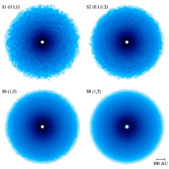
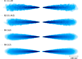
Figure 1: Disc morphology: volume gas density in midplane and vertical cross sections for simulations S1, S2, S6, S8 (from top to bottom and from left to right). The values of the two AV parameters ($\alpha,\beta$) are displayed for each case.

3 Diagnostics and reference values for PPD

We consider two kinds of diagnostics which refer to the global flow and to fluctuations of several quantities, with particular focus on density and velocity field. We first define the diagnostic and then give the expected values in some known cases. In the following, the symbol $\langle\cdot\rangle$ represents average quantities. In this paper we perform both the standard azimuthal and vertical averages $\langle\cdot\rangle_{\theta z}$ and the azimuthal averages only $\langle\cdot\rangle_{\theta}$, in order to characterise also the vertical extension.

3.1 Diagnostic for the global disc flow

Here, we present the selected quantities used to characterise the global flow.

1. Mass distribution. We look at:

   1. the radial profile of the surface density $\Sigma(R)$,

   2. the density distribution $\rho(R_{\mathrm{s}},z)$ in the direction perpendicular to the disc midplane, for a selected radius $R_{\mathrm{s}}$.

2. Velocity structure. We focus on:

   1. the radial velocity maps $v_{R}(R,z)$, where the radial component of the velocity field is azimuthally averaged.

   2. the local Mach number of the flow in the midplane Ma$(R)\equiv v(R)/c_{\mathrm{s}}(R)$, where $v$ is the modulus of the local velocity field.

3. Macroscopic turbulence signatures. Four items are analysed.

   1. The mass accretion rate onto the central star $\dot{M}_{0}$: we are particularly interested in this quantity for two reasons: (1) it gives indirect information about the turbulent viscosity coefficient and (2) it is constrained by observations. For PPD around T Tauri stars the measured values of mass accretion rates onto the central star are $\dot{M}\approx 10^{-8}$ M_⊙ (Hartmann et al., 1998; Andrews et al., 2009), they can be reproduced by a value $\alpha_{\mathrm{\scriptstyle{ss}}}\approx 10^{-2}$ (Hartmann et al., 1998; King et al., 2007).

   2. Since $\dot{M}_{0}$ gives an information restricted to the very inner region of the disc (where our inner boundary condition is free), we also analyse the radial profile of the local mass accretion rate: $\dot{M}(R)=-2\pi R\Sigma\langle v_{R}\rangle_{\theta z}$, averaged in the azimuthal and vertical direction.

   3. The effective viscosity $\alpha_{\mathrm{\scriptstyle{eff}}}$ of the gaseous disc (we express the viscosity in terms of the dimensionless parameter $\alpha_{\mathrm{\scriptstyle{ss}}}$ of the SS73 parametrization) that characterises the simulated disc.

      The effective viscosity in the simulated disc model is estimated by means of fits to the two-dimensional analytic models of accretion discs (see details in Appendix B). We use 2D analytic models because they are well suited for the azimuthal symmetry present in our simulated discs. For this reason we call $\alpha_{\mathrm{\scriptstyle{2D}}}$ this way of estimating the effective viscosity $\alpha_{\mathrm{\scriptstyle{eff}}}$. In particular, we derive $\alpha_{\mathrm{\scriptstyle{2D}}}$ by comparing the vertical profile of the radial velocity of the gas flow to the expression derived by analytic $\alpha_{\mathrm{\scriptstyle{ss}}}$-disc models for different radial positions. We rewrite the vertical profile of the radial velocity, given by TL02 and Fromang et al. 2011, highlighting the scale height of the disc $H(R)$ at radial position $R$:

      $$\frac{v_{R}}{c_{\mathrm{s_{0}}}}= \ \frac{\alpha_{\mathrm{\scriptstyle{2D}}}}{2}\frac{H(R)}{R_{0}}\left(\frac{R}{R_{0}}\right)^{-\frac{1+q}{2}}\times$$ (15)

      $$\ \left\{6p+q-3-(9-5q)\left[\frac{z}{H(R)}\right]^{2}\right\}.$$

      Lodato & Price (2010) estimated $\alpha_{\mathrm{\scriptstyle{eff}}}$ by fit of the surface density profile of 1D viscous accretion discs (Pringle, 1981) and found good agreement with $\alpha_{\mathrm{\scriptstyle{cont,Mu96}}}$ in SPH simulations of warped discs when the necessary equivalence conditions (large number of particles and Mu96 artificial viscosity, see Sect. 2.1.2) are met.

   4. Once we know the effective viscosity of the disc, we can derive the corresponding Reynolds number:

      $$\mathrm{Re}_{\mathrm{\scriptstyle{eff}}}=\frac{\mathrm{Ma}}{\alpha_{\mathrm{\scriptstyle{eff}}}}.$$ (16)

3.2 Diagnostic for fluctuations

For each simulated disc we have studied both the magnitude and the structure of the fluctuations present in the disc with particular attention to the velocity field. Since current observations have not yet reached the resolution necessary to directly detect turbulence and study its features in protoplanetary discs (some progress has been recently claimed by Hughes et al. 2011 and Guilloteau et al. 2012, who measured some turbulent velocities in mm observations) the resulting properties of density and velocity fluctuations have been compared to the typical behaviour observed in turbulence experiments and to results from grid- and particle-based simulations available in the literature.

The components of the velocity field are identified by $v_{i}$ and those of the fluctuating velocity field are $u_{i}=v_{i}-\langle v_{i}\rangle$ with $i=R,\theta,z$.

3.2.1 Magnitude of velocity fluctuations

Concerning the magnitude of velocity fluctuations, we focus on the turbulent viscosity coefficient (point M1), the diffusion coefficients (point M2) and the Mach number of velocity fluctuations (point M3).

1. The turbulent viscosity coefficient $\nu_{\mathrm{\scriptstyle{T}}}$ is often derived from Reynolds averages of Navier-Stokes equations with the turbulent viscosity hypothesis (e.g. Pope, 2000) and is thus related to Reynolds stresses:

   $$\nu_{\mathrm{\scriptstyle{T}}}=-\langle u_{R}u_{\theta}\rangle_{\theta}\left/\left[R\frac{\partial\left(\langle v_{\theta}\rangle_{\theta}/R\right)}{\partial R}\right]\right.$$ (17)

   (see Appendix A.1).

   Here we call $\alpha_{\mathrm{\scriptstyle{RS}}}$ the corresponding SS73 parameter for a disc in quasi-Keplerian rotation, it is given by:

   $$\alpha_{\mathrm{\scriptstyle{RS}}}(R,z)=\frac{2}{3}\frac{\langle u_{R}u_{\theta}\rangle_{\theta}}{c_{\mathrm{s}}^{2}},$$ (18)

   where Eq. 17 has been combined with the SS73 relation $\nu_{\mathrm{\scriptstyle{T}}}$ = $\alpha_{\mathrm{\scriptstyle{ss}}}c_{\mathrm{s}}H$ (see Appendix A.2). For each radial and vertical position, averages are performed spatially along the azimuthal direction in order to be able to derive the radial and vertical dependence of $\alpha_{\mathrm{\scriptstyle{RS}}}$.

   The corresponding turbulent Reynolds number is:

   $$\mathrm{Re}_{\mathrm{\scriptstyle{T}}}=\frac{\mathrm{Ma}}{\alpha_{\mathrm{\scriptstyle{RS}}}}.$$ (19)

   In MHD simulations of accretion discs, $\alpha_{\mathrm{\scriptstyle{ss}}}\approx 10^{-3}$ and includes both the Reynolds and Maxwell stresses (e.g. Fromang & Nelson, 2009; Flock et al., 2012), in simulations of self-gravitating discs, $\alpha_{\mathrm{\scriptstyle{ss}}}\approx 10^{-2}$ and includes both the Reynolds and gravitational stresses (e.g. Rice et al., 2005; Rice et al., 2011).

2. Turbulent flows are often approximated by means of models where turbulence is described as a diffusive process. Here we want to determine if diffusion is present in our simulations. To this end the method used by Fromang & Papaloizou (2006) in order to calculate the turbulent diffusion coefficient $D_{\mathrm{\scriptstyle{T}}}$ is well suited for Lagrangian codes such as SPH:

   $$D_{\mathrm{\scriptstyle{T}}}(t)=\int_{0}^{t}S_{zz}(t^{\prime})\mathrm{d}t^{\prime}$$ (20)

   where $S_{zz}$ is the vertical velocity correlation function:

   $$S_{zz}(t)=\langle v_{z}(z,t)v_{z}(z_{0},0)\rangle,$$ (21)

   with $z_{0}$ representing the vertical position of a given particle at time $t=0$ and $z$ the vertical position of the same particle at time $t$; in a similar way $v_{z}(z_{0},0)$ is the velocity of the same particle at time $t=0$ and $v_{z}(z,t)$ at time $t$. In order to compute the diffusion coefficient at a selected radial location $R_{\mathrm{s}}$, we average the diffusion coefficient of single particles that were at $R_{\mathrm{s}}$ at the beginning of the simulation.

   A diffusion coefficient $D_{\mathrm{\scriptstyle{T}}}/(c_{\mathrm{s}}H)\approx 5\cdot 10^{-3}$ is found by Fromang & Papaloizou (2006) in MHD local shearing box stratified simulations.

3. The strength of velocity fluctuations and therefore their subsonic or supersonic behaviour can be determined by the corresponding Mach number, defined as the ratio of the modulus of velocity fluctuations to the gas sound speed:

   $$\mathrm{Ma}_{\mathrm{f}}\equiv\frac{|u|}{c_{\mathrm{s}}}.$$ (22)

   We have computed azimuthal-only and azimuthal and vertical averages in order to present $R$–$z$ maps and radial profiles.

   In the global MHD simulations of stratified discs of Fromang & Nelson (2006) and Flock et al. (2011), the Mach number of velocity fluctuations is $\mathrm{Ma}_{\mathrm{f}}\approx 0.1$ around the midplane and $\mathrm{Ma}_{\mathrm{f}}\approx 0.4$ in the surface layers.

3.2.2 Structure of velocity fluctuations

Concerning the structure of velocity fluctuations, we focus on the anisotropy vector (point S1), on the power spectrum (point S2) and on the possible presence of intermittency (point S3).

1. In order to determine the isotropic or anisotropic character of velocity fluctuations, we define the anisotropy vector $\vec{\delta}$ = $(\delta_{R},\delta_{\theta},\delta_{z})$ in terms of the velocity dispersion in the three spatial directions, in analogy with galactic dynamics (see e.g. Bertin, 2000):

   $$\delta_{i}\equiv 2-\frac{\sigma_{j}^{2}+\sigma_{k}^{2}}{\sigma_{i}^{2}},$$ (23)

   where the square of the velocity dispersion $\sigma_{i}^{2}$ = $\langle(v_{i}-\langle v_{i}\rangle)^{2}\rangle$ = $\langle u_{i}^{2}\rangle$ = $\langle v_{i}^{2}\rangle-\langle v_{i}\rangle^{2}$ and $i$, $j$ and $k$ refer to the three cylindrical components. Systems with anisotropy in the $i$ direction are characterised by a velocity dispersion of the $i$ component that is larger than that of the other two components: $\sigma_{i}\gg\sigma_{j}$ and $\sigma_{i}\gg\sigma_{k}$. Therefore, the $i$ component of the anisotropy vector will be $\delta_{i}\approx 2$. Averages are performed along both the vertical and the azimuthal direction.

   From the plots of Fromang & Nelson (2006) and Flock et al. (2011) we can deduce that $\sigma_{R}\gg\sigma_{\theta}\approx\sigma_{z}$, therefore MHD discs are radially anisotropic and the corresponding anisotropy vector is $\vec{\delta}\approx(2,0,0)$. In contrast, in experiments of turbulence produced by round jets a corresponding azimuthal anisotropy $\vec{\delta}\approx(0,2,0)$ has been observed (e.g. Pope, 2000).

2. The power spectrum is computed along a ring of selected radius $R_{\mathrm{s}}$, centred on the star and located at the selected vertical position $z_{s}$ (see Appendix A.3):

   $$P_{i}(R_{\mathrm{s}},z_{s};k)=|\hat{u}_{i}(k)|^{2},$$ (24)

   with $\hat{u}_{i}(k)$ the Fourier transform of the component $i$ of the velocity fluctuation vector and $k=1/\lambda$ the wavenumber corresponding to length scale $\lambda$. We analyse the power spectrum of the velocity field in order to determine if an energy cascade, characteristic of turbulent systems, is present and if differences related to the position inside the disc are relevant.

3. Highly turbulent flows are characterised by intermittency (e.g. Frisch, 1996). This feature implies non-Gaussian probability distribution functions (PDFs) with corresponding non-Gaussian higher order moments. Here we focus on the density and acceleration PDFs and on their $3^{rd}$ (skewness, noted $S$) and $4^{th}$ (kurtosis, noted $K$) order moments (see Appendix A.3).

Data are not available for the power spectrum of fluctuations and for the phenomenon of intermittency in accretion discs. In the classical Kolmogorov theory of incompressible homogeneous turbulence the power spectrum of velocity fluctuations has a power law form $P(k)\sim k^{s}$ with $s$ = $-5/3$. Recent simulations of supersonic compressible gas found a slope of $s$ $\approx$ $-2$ (Price & Federrath, 2010, and references therein). Intermittency, highlighted by non-Gaussian PDFs and higher order moments, is experimentally found in very high Reynolds number incompressible flows. In SPH simulations of a simple weakly compressible periodic shear flow, Ellero et al. (2010) find that the PDF of the particle acceleration is in good agreement with non-Gaussian statistics observed experimentally for incompressible flows.

In simulations of supersonic compressible turbulence (see e.g. Price & Federrath, 2010), log-normal distributions of the density PDF have been observed:

$$p(x)=\frac{1}{\sqrt{2\pi\sigma_{p}^{2}}}\exp\left[-\frac{(x-\langle x\rangle)^{2}}{2\sigma_{p}^{2}}\right]$$ (25)

with $x=\textrm{ln}(\rho/\langle\rho\rangle)$ and a width controlled by the Mach number of the fluctuations

$$\sigma_{p}^{2}=\textrm{ln}\left(1+b^{2}\textrm{Ma}^{2}\right),$$ (26)

where $b\approx 0.5$. The expressions of the skewness and kurtosis in terms of $\sigma_{p}$ for the log-normal distribution are

$$\left\{\begin{array}[]{r c l}S&=&\left(\textrm{e}^{\sigma_{p}^{2}}+2\right)\sqrt{\textrm{e}^{\sigma_{p}^{2}}-1}\\ K&=&\textrm{e}^{4\sigma_{p}^{2}}+2\textrm{e}^{3\sigma_{p}^{2}}+3\textrm{e}^{2\sigma_{p}^{2}}-3.\end{array}\right.$$ (27)

When $\sigma_{p}\rightarrow 0$ the log-normal distribution tends to a Gaussian distribution and the skewness and kurtosis tend to their gaussian values (0 and 3 respectively).

The results of the application of these diagnostics to the simulations we performed are described in Sects 4, 5 and 6.

4 The disc global flow

We now consider how the main properties of the global disc flow (mass distribution, velocity structure, mass accretion rate and effective disc viscosity) depend on the strength of artificial viscosity. The convergence of each quantity is also studied.

4.1 Mass distribution

The position of the peak of the surface density profile $\Sigma(R)$ moves towards larger radial distances and its maximum decreases (see left panel of Fig. 2), when the two AV parameters $\alpha$ and $\beta$ are increased: such behaviour is in agreement with the viscous spreading mechanism that is expected here due to the existing correlation between artificial and physical viscosity (see Sect. 2.1.2).

An increase in resolution (see right panel of Fig. 2) has a qualitatively similar effect to a decrease in viscosity: the surface density peak moves towards the centre of the disc, becoming higher (note also that the curve becomes less noisy). In the central and external regions the projected density profile converges already for a number of particles as small as $5\cdot 10^{4}$. In the inner region ($R<10^{-1}R_{out}$), a trend towards convergence is present, but a higher number of particles, $N\gtrsim 10^{6}$, is necessary.

The vertical density profile $\rho(R_{\mathrm{s}},z)$ at a selected radius $R_{\mathrm{s}}$ (see insets in Fig. 2 for $R_{\mathrm{s}}=1$) follows the expected Gaussian distribution of Eq. 9, showing that the desired profile is well reproduced by the sampling procedure and by numerical thermalisation. It is not significantly affected by changing $\alpha$, $\beta$ or $N$.

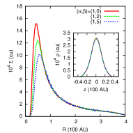
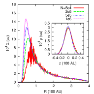
Figure 2: Mass distribution. Dependence of the surface density $\Sigma(R)$ and vertical density profile $\rho(R_{\mathrm{s}}=1,z)$ on the AV parameters (left: simulations S6, S7, S8, S9 with $N=2\cdot 10^{5}$ particles) and on the resolution (right: simulations S21, S8, S23, S24 with ($\alpha$,$\beta$)=(1,5)). Values are given in code units.

4.2 Velocity structure

4.2.1 Radial velocity maps

Maps of the azimuthally averaged radial velocity $\langle v_{R}\rangle_{\theta}$ in the $R$-$z$ plane are displayed in Figs. 3 and 4 for changing artificial viscosity and resolution respectively.

Effect of artificial viscosity parameters. A transition from a chaotic to a regular accretion pattern is clearly observed in Fig. 3 when $\alpha$ is increased for a given $\beta$ (panels from top to bottom) and as well as when $\beta$ is increased for a given $\alpha$ (panels from left to right).

At large radii, a well extended decretion region dominates in all models, as expected from the conservation of angular momentum. At smaller radii, instead, the structure of the gas flow strongly depends on the values of the AV parameters. A decretion flow located around the midplane, associated with an accretion flow in thin surface layers, appears when $(\alpha,\beta)$ are increased. Such accretion layers become thicker for larger AV parameters. Therefore, the gas flow is characterised by the phenomenon of meridional circulation. This mechanism has been found in some two-dimensional viscous disc models (e.g. TL02 that extends the standard one dimensional SS73 models to two dimensions: radial and vertical) but is not reproduced by MHD disc simulations where turbulence is induced by the MRI (Fromang et al., 2011; Jacquet, 2013). The presence of meridional circulation has important implications for the topic of particle mixing in PPD and is one of the possible mechanisms able to explain the presence of crystalline solid particles in the outer regions of T Tauri stars recently observed by Spitzer (e.g. Sargent et al., 2009). Finally, in the very inner region of the disc a small and well defined accretion region is present in all models.

Effect of artificial viscosity implementation. The two panels in the bottom row of Fig. 4 show the structure of the radial velocity flow of two discs at different resolution simulated with the Mu96 artificial viscosity. The resulting flow structure can be directly compared with the panel above, which represents the flow structure in an equivalent disc at the same resolution but simulated with the MG83 artificial viscosity. In the simulations at lower resolution ($N=2\cdot 10^{5}$), the meridional circulation pattern is better reproduced by the MG83 implementation. However, in the more resolved discs ($N=10^{6}$) the two patterns are very similar. The two small accretion regions present in the outer Mu96 discs are due to a longer relaxation time-scale for this particular artificial viscosity implementation (in longer evolution simulations, not shown here, we have observed a net outward gas flow in agreement with the MG83 case and the expected viscous spreading).

Effect of resolution. The first row in Fig. 4 shows how the radial velocity structure has already converged after $N\approx 5\cdot 10^{5}$ particles.

TL02 found that the outflow zone around the midplane shrinks as the radial volume density gradient is reduced ($s\rightarrow 0$) and when the condition $p+q<2$, that guarantees a net accretion of the gas onto the star, is violated. Therefore, we expect that the thickness of the accretion layers depends on the values ($p$, $q$) of the surface density and temperature radial profiles of the gaseous disc model. However, a detailed study of the dependence of the structure of the accretion layers on the gas density and temperature profiles and the correlation with the central mass accretion rate is out of the scope of this paper and will be addressed in a future work. For the initial profile of the disc model used in this work we have $p+q=2.25$, which implies net decretion but is very close to the limit between net accretion and decretion. The surface density of the simulated discs after numerical relaxation reaches a smooth profile that, in the inner region, is slightly shallower (implying a slightly smaller $p$) than the initially imposed power law, which is characterised by an inner sharp edge (see Sect. 2.2). This moves the model in the net accretion region and explains the presence of the observed thin accretion layers.

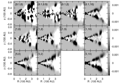
Figure 3: Radial velocity structure of the gaseous disc: changing AV parameters. Maps of the azimuthally averaged radial velocity $\langle v_{R}(R,z)\rangle_{\theta}$ in the meridian plane for simulations with $N=2\cdot 10^{5}$ particles and the MG83 artificial viscosity implementation. The colorbar gives the radial velocity: negative values correspond to gas inflow and positive values to outflow. Values of ($\alpha$,$\beta$) are given in each subplot.

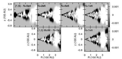
Figure 4: Radial velocity structure of the gaseous disc: changing resolution and artificial viscosity implementation. The layout is the same as in Fig. 3. The top row shows how the radial velocity structure changes with resolution for simulations with the MG83 artificial viscosity, the specific case of simulations with ($\alpha$,$\beta$)=(1,5) has been chosen as an example: panels from left to right correspond respectively to $N$=$5\cdot 10^{4}$, $2\cdot 10^{5}$, $5\cdot 10^{5}$, $1\cdot 10^{6}$. The bottom row refers to two simulations with the Mu96 artificial viscosity implementation (with $\alpha=1$) and with $N$=$2\cdot 10^{5}$ (left panel) and $N$=$1\cdot 10^{6}$ (right panel).

4.2.2 Mach number of the flow

The gas in the disc is supersonic. In fact, since the gas moves on quasi-Keplerian orbits, the Mach number is approximated by Ma $\approx v_{\mathrm{k}}/c_{\mathrm{s}}$. With the adopted sound speed profile it becomes: Ma $\approx R^{(q-1)/2}/c_{\mathrm{s}0}$. For the values used here Ma $\approx 20R^{-1/8}$, which is approximately in the range of values 15–25.

4.3 Mass accretion rate

The mass accreted onto the central star (Fig. 5) and the radial profiles of the mass accretion rate (Figs. 6 and 7) are two macroscopic signatures of turbulence.

4.3.1 Central mass accretion rate

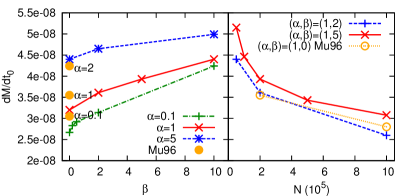
Figure 5: Central mass accretion rate $\dot{M}_{0}$. Left panel: dependence on the AV parameters for a given number of particles ($N=2\cdot 10^{5}$), Right panel: dependence on resolution. The mass accretion rate is displayed in units of $M_{\odot}\textrm{yr}^{-1}$.

Effect of artificial viscosity. The left panel in Fig. 5 shows that $\dot{M}_{0}$ increases with larger $\alpha$ and/or larger $\beta$ and in the case of the Mu96 artificial viscosity implementation. The effect of $\alpha$ is larger, as expected since it controls the first order in the artificial viscosity term.

Effect of resolution. The right panel in Fig. 5 shows that $\dot{M}_{0}$ decreases with increasing resolution. Such an effect is due to a decrease of particle noise at higher resolution, which decreases the numerical dissipation. This is linked to the dependence of the effective viscosity on resolution (see Sect. 4.4). In fact, as will be shown in Sect. 6.3.1, the PDFs of several physical quantities are narrower at higher resolution, due to the reduced noise. Concerning the central mass accretion rate we look at the part of the radial velocity distribution corresponding to negative velocities, since only fluid elements with negative radial velocity are responsible for accretion. The radial velocity distribution at higher resolution presents a smaller spread than in the lower resolution case. In addition, SPH particles in low resolution simulations have a larger mass than in higher resolution simulations. Therefore, at lower resolution there is a larger number of more massive SPH particles with higher inward radial velocity, implying higher accretion rates. The trend of the curve shows that the central accretion rate is converging, however convergence is not yet reached at one million particles.

For all the considered combinations of ($\alpha$,$\beta$) and $N$, we find mass accretion rates consistent with the values observed for PPD. In addition, we observe a correlation between the trend of $\dot{M}_{0}$ with respect to $(\alpha$, $\beta)$ and the increase of thickness of the accreting layers (net accreting mass flux) observed in Fig. 3. Similarly, the trend with respect to $N$ correlates with the decrease of thickness of the accreting layers at higher resolution, observed in Fig. 4.

4.3.2 Radial profile of the mass accretion rate

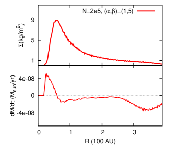
Figure 6: Gas flow in the disc. Surface density radial profile (top panel) and mass accretion rate radial profile (bottom panel) for simulation S8.

The central mass accretion rate $\dot{M}_{0}$ gives information only about the region of the disc that is close to the star. In order to have a global picture of the mass flux in the disc, it is interesting to look at the radial profile of the vertically integrated mass accretion rate $\dot{M}(R)$. As an example, the profile observed in simulation S8 is displayed in the bottom panel of Fig. 6. The flow is characterised by an inner accreting region separated, at a radius we call $R_{t}$, from an outer decreting region with small rates at intermediate radii and larger rates at large radii. It can be understood by a comparison to the surface density profile (top panel of Fig. 6). In the organized flow of model S8, $R_{t}$ corresponds to the radial location of the surface density peak, which moves outwards with time due to viscous spreading, as the density maximum decreases. The density peak behaves as a reservoir of gas that supplies mass both to the inwards and outwards flows, resulting in an apparent null mass accretion rate at $R_{t}$. The varying rate in the decretion region is due to the vertical structure of the flow: Fig. 3 shows accretion throughout the disc height for the inner disc, accretion in the midplane with decretion in the surface layers at intermediate radii resulting in a slightly negative radial mass flux, and decretion throughout the disc height in the very outer regions.

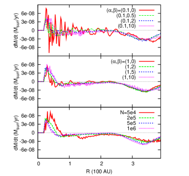
Figure 7: Radial profiles of the mass accretion rate. The effect of artificial viscosity is shown for $\alpha=0.1$ (top panel) and 1 (middle panel) and changing $\beta$, for simulations with $N=2\cdot 10^{5}$ particles. The effect of resolution is displayed in the bottom panel for simulations with $(\alpha,\beta)=(1,5)$.

Effect of artificial viscosity. For low values of $\alpha$ and $\beta$ fluctuations are so large that the identification of an organized flow of the fluid is not possible. As shown by the top panel of Fig. 7, the mass accretion rate profile is very noisy with a narrow peak in the inner disc, an average value close to zero in the intermediate regions and negative in the outer disc. The peak of the surface density profile decreases with time but less than in the higher $(\alpha,\beta)$ case and it does not change position with time. In the $v_{R}$ map (see the top left corner of Fig. 3) negative and positive regions are clearly mixed.

Increasing the two AV parameters, the profile becomes more regular and smooth, following the structure described above for the specific simulation S8. For $\alpha$ = $1$ the profile tends to converge when $\beta$ is increased (see the middle panel). In the Mu96 case we observe similar radial profiles for the mass accretion rate (not shown).

Effect of resolution. As shown in the bottom panel of Fig. 7 for the simulations with $(\alpha,\beta)=(1,5)$ and increasing resolution, the peak of the radial profile of the mass accretion rate moves inwards and converges for $N\ga 5\cdot 10^{5}$, in agreement with the convergence observed for the radial velocity maps. The reason of the decrease of the peak in higher resolution simulations is the same that explains the similar decreases observed for the central mass accretion rate (see Sect. 4.3.1).

4.4 The effective viscosity of the SPH disc: $\alpha_{\mathrm{\scriptstyle{2D}}}$

In order to estimate the effective viscosity of the gaseous disc, we determine the $\alpha_{\mathrm{\scriptstyle{2D}}}$ parameter, which is derived by fitting the vertical profile of the radial velocity expected for a viscous axisymmetric accretion disc, given by Eq. 15, to that derived from the simulations (see Appendix B for the fitting procedure). Two examples, characterised by adequately large AV parameters, are shown in Fig. 8, where the vertical profile of the radial velocity at radial position $R=1$ is displayed for simulation S7 (top panel) and for simulation S20 (bottom panel).

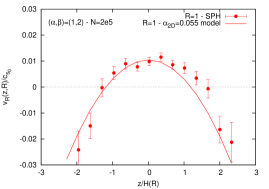
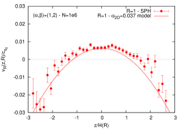
Figure 8: Determination of $\alpha_{\mathrm{\scriptstyle{2D}}}$. The vertical profile of the radial velocity extracted from simulations (points with error bars) is fitted by the two-dimensional $\alpha_{\mathrm{\scriptstyle{SS}}}$-disc model (solid lines). Top: simulation S7, bottom: simulation S20.

In Fig. 9 we present the values of $\alpha_{\mathrm{\scriptstyle{2D}}}$ obtained by averaging the result of the fit at $R$=1 and $R$=2 for the set of simulated discs. The values are averaged in the radial range $[1,2]$. In simulations with $\alpha=0.1$ the vertical profile of radial velocity cannot be described by the profile in Eq. 15 because the high noise level makes the fit impossible. We find that simulation profiles can be fitted by a value of $\alpha_{\mathrm{\scriptstyle{2D}}}$ which is roughly the same for the different radial locations we considered. This shows that the structure of SPH models is consistent with the 2D version of SS73 accretion disc models, characterised by a constant $\alpha_{\mathrm{\scriptstyle{ss}}}$ value.

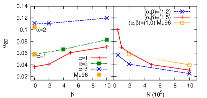
Figure 9: Results for $\alpha_{\mathrm{\scriptstyle{2D}}}$. The parameter has been determined by averaging the values fitted at $R$=1 and 2 and only for simulations where the noise is low enough to allow the fit.

Effect of artificial viscosity. In the range of AV parameters were the determinations of the effective viscosity is possible ($\alpha>0.1$), the scaling of $\alpha_{\mathrm{\scriptstyle{2D}}}$ with the AV parameters (increase with larger $\alpha$ and/or $\beta$ in the MG83 implementation and increase with larger $\alpha$ for the Mu96 implementation) has the same qualitative behaviour as for the central mass accretion rate (see Fig. 5). Such a match is what we expect, since a more viscous disc is characterised by a larger central accretion rate. The weaker dependence on $\beta$ is in agreement with the fact that $\beta$ is the parameter controlling the second order term of the MG83 artificial viscosity (see Eq. 4).

Effect of resolution. The trend of the curves in the right panel of Fig. 9 is qualitatively similar to that of the central mass accretion rate (see Fig. 5) and shows that the effective viscosity is converging. However one million particles is still not enough in order to reach convergence. The slightly higher resolution required for the convergence of $\alpha_{\mathrm{\scriptstyle{2D}}}$ and $\dot{M}_{0}$ with respect to that required by the radial velocity maps and by the mass accretion rate radial profile ($N\approx 5\cdot 10^{5}$) is due to the fact that the former two parameters are calculated from a smaller subset of simulation particles, the numerical noise is therefore larger.

The result of this subsection is that the effective viscosity $\alpha_{\mathrm{\scriptstyle{2D}}}$ in all the SPH models considered here equals a few $10^{-2}$, in agreement with the order of magnitude deduced from observations.

4.4.1 Reynolds number

Once the effective viscosity of the disc is determined ($\alpha_{\mathrm{\scriptstyle{eff}}}\approx\alpha_{\mathrm{\scriptstyle{2D}}}$), it becomes possible to derive the corresponding Reynolds number $\mathrm{Re}_{\mathrm{\scriptstyle{eff}}}\approx\mathrm{Re}_{\mathrm{\scriptstyle{2D}}}=\mathrm{Ma}/\alpha_{\mathrm{\scriptstyle{2D}}}$, shown in Fig. 10. In accordance with the trend of $\alpha_{\mathrm{\scriptstyle{2D}}}$ with respect to $\alpha$, $\beta$ and $N$, described in the last paragraph, we found larger Re numbers in less viscous and more resolved discs.

Simulations with one million particles and the MG83 artificial viscosity are closer to, but sill lower than the value $\mathrm{Re}_{\mathrm{\scriptstyle{eff}}}\approx 3\cdot 10^{3}$, which is considered as a limit for the onset of the turbulent regime in a box with periodic boundaries (see Price, 2012). Therefore, the dynamics of the discs presented in this paper is not expected to be dominated by fully-developed turbulence.

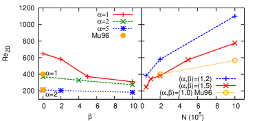
Figure 10: The effective Reynolds number: $\mathrm{Re}_{2D}$. Derived from the effective viscosity presented in Fig. 9.

4.4.2 The $\alpha_{\mathrm{\scriptstyle{2D}}}$-$\alpha_{\mathrm{\scriptstyle{cont}}}$ connection

Figure 11 shows the relation between the effective viscosity $\alpha_{\mathrm{\scriptstyle{2D}}}$ (computed in the simulations) and the $\alpha_{\mathrm{\scriptstyle{cont}}}$ viscosity (expected when the continuum limit of the SPH equations is taken) for eight of the performed simulations with $\beta=0$ (S6, S10, S13, S17, S18, S25, S27). Simulations S1 and S16 (with $\alpha=0.1$) are too noisy to allow the determination of $\alpha_{\mathrm{\scriptstyle{2D}}}$. Since the ratio $\langle h\rangle/H$ in the expression of $\alpha_{\mathrm{\scriptstyle{cont}}}$ depends on the radial location inside the disc (see Eqs. 7 and 8), we have evaluated locally at the radial position $R=1$ both $\alpha_{\mathrm{\scriptstyle{cont}}}$ and $\alpha_{\mathrm{\scriptstyle{2D}}}$, whose values are given in Table 3.

We find that both the points concerning the Mu96 case and those concerning the MG83 case follow the appropriate analytic relation. We therefore confirm the necessity of reducing the coefficient in the $\alpha_{\mathrm{\scriptstyle{cont}}}$ relation in Eq. 8 for the MG83 case as shown by Meru & Bate (2012) and motivated by the fact that in the MG83 implementation the artificial viscosity is applied only to approaching particles.

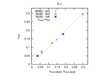
Figure 11: Comparison of the the effective viscosity of the disc $\alpha_{\mathrm{\scriptstyle{2D}}}$ with the corresponding $\alpha_{\mathrm{\scriptstyle{cont}}}$ formula: simulations S6, S10 and S13 (MG83, $N$=$2\cdot 10^{5}$), S17, S18 and S27 (Mu96, $N$=$2\cdot 10^{5}$) and S25 and S26 (Mu96, $N$=$10^{6}$). The displayed values are computed at the radial position $R=1$. The dotted line represents identity between $\alpha_{\mathrm{\scriptstyle{cont}}}$ and $\alpha_{\mathrm{\scriptstyle{2D}}}$. Error bars are comparable to the symbol sizes and are not displayed, their values are given in Table 3.

Finally, no significant difference is observed when resolution is changed from $2\cdot 10^{5}$ to $10^{6}$ particles, suggesting that already with $2\cdot 10^{5}$ particles the continuum approximation can be considered valid.

Table 3: Error bars associated to $\alpha_{2D}$ produced by the fitting procedure.

Simulation	$\alpha_{cont}$	$\alpha_{2D}$
S6	0.0301	0.0490 $\pm$ 0.0063
S10	0.0597	0.0668 $\pm$ 0.0040
S13	0.1476	0.1453 $\pm$ 0.0023
S17	0.0601	0.0759 $\pm$ 0.0043
S18	0.1204	0.1249 $\pm$ 0.0033
S27	0.3009	0.2949 $\pm$ 0.0075
S25	0.0372	0.0500 $\pm$ 0.0013
S26	0.1852	0.1776 $\pm$ 0.0009

5 The magnitude of SPH fluctuations

5.1 The Reynolds stress contribution to the SPH disc viscosity: $\alpha_{\mathrm{\scriptstyle{RS}}}$

We now proceed with the determination of $\alpha_{\mathrm{\scriptstyle{RS}}}$, which is the $\alpha_{\mathrm{\scriptstyle{SS}}}$ parameter derived from the Reynolds stress, in analogy with turbulence studies and with MHD or self-gravitating disc simulations. Radial and azimuthal fluctuations are computed from the average velocity field determined locally using a $R$–$z$ grid.

The radial profile of the vertically averaged $\alpha_{\mathrm{\scriptstyle{RS}}}$ is shown in the left panel of Fig. 12, where the effect of changing $\alpha$ and $\beta$ is highlighted, and of Fig. 13, where the effect of resolution is shown. In all simulations, the coefficient $\alpha_{\mathrm{\scriptstyle{RS}}}$ is characterised by a similar profile: it tends to be approximately constant throughout the radial extension of the disc, with an increase both in the central and in the external radial region.

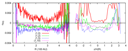
Figure 12: Radial (left) and vertical (right) profiles of $\alpha_{\mathrm{\scriptstyle{RS}}}$. Effect of changing the AV parameters.

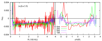
Figure 13: Radial (left) and vertical (right) profiles of $\alpha_{\mathrm{\scriptstyle{RS}}}$. Effect of changing the resolution.

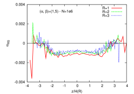
Figure 14: Vertical profiles of $\alpha_{\mathrm{\scriptstyle{RS}}}$. Comparison at three different radial location in the disc for simulation S24.

The right panel of both figures shows the radially averaged vertical profile (as in Fig. 8, the semi-thickness of the disc is computed from $H(R)$=$H_{0}(R/R_{0})^{(3-q)/2}$, see Sect. 2.2): $\alpha_{\mathrm{\scriptstyle{RS}}}$ is approximately constant around the midplane and then increases with height. This behaviour qualitatively agrees with that observed in MHD discs by Flock et al. (2011), even if we observe a broader minimum. In addition, we have found that the vertical profile is approximately the same at different radial positions, as shown in Fig. 14 for simulation S24.

Effect of artificial viscosity. The radial and vertical profiles of $\alpha_{\mathrm{\scriptstyle{RS}}}$ are very sensitive to the AV parameters $\alpha$ and $\beta$. In fact there is a sharp change in the average value, which decreases from positive to negative values, when the two AV parameters are increased. This transition is clearly visible in both panels of Fig. 12 for $\alpha=1$: the increase of $\beta$ from 0 to 2 shifts the profile of $\alpha_{\mathrm{\scriptstyle{RS}}}$ towards smaller values, moving it in the negative region. A further increase of $\beta$ leads to smaller changes, but the behaviour inverts: higher artificial viscosity now tends to increase the value of the coefficient $\alpha_{\mathrm{\scriptstyle{RS}}}$ (which corresponds to a decrease of its absolute value, see left panel) and to extend the constant region around the midplane (see right panel). We find the same trend for other values of $\alpha$ (not shown).

The change of sign of $\alpha_{\mathrm{\scriptstyle{RS}}}$ is due to the mechanism of meridional circulation that is correctly resolved when adequately high AV parameters are used.

Effect of resolution. For a given combination of AV parameters, the radial and vertical profiles of the $\alpha_{\mathrm{\scriptstyle{RS}}}$ coefficient do not change with resolution. The only effect of increasing the number of particles of the simulation is a reduction of the noise, which implies smoother profiles.

We note that the computation of $\alpha_{\mathrm{\scriptstyle{RS}}}$ is very sensitive to the correct determination of the average velocity field of the flow, therefore only in simulations with adequately high values of $\alpha$ and $\beta$, where numerical noise and particle disorder are lower, can it be trusted. The absolute value of $\alpha_{\mathrm{\scriptstyle{RS}}}$ for the present simulations is $|\alpha_{\mathrm{\scriptstyle{RS}}}|\approx 10^{-3}$. This is comparable to standard values found in MHD discs (see e.g. Fromang & Nelson, 2006). The difference is that meridional circulation is present here and the negative value indicates decretion on average in the midplane, in contrast to the positive value of MHD discs (where meridional circulation is not seen), which is expected for accretion in the midplane.

In conclusion, more viscous discs are characterised by a smaller modulus of $\alpha_{\mathrm{\scriptstyle{RS}}}$ and, for all the simulations we performed, we find the ratio of the Reynolds stress to the effective viscosity of the gaseous disc to be $\alpha_{\mathrm{\scriptstyle{RS}}}/\alpha_{\mathrm{\scriptstyle{2D}}}$ $\approx$ $10^{-1}$. This means that velocity fluctuations are not the main component of the effective viscosity of the disc, in agreement with the low Reynolds number of the global flow in in the present simulations (see Sect. 4.4.1). However, the turbulent Reynolds number, which is associated to the Reynolds stress, amounts to $\mathrm{Re}_{\mathrm{\scriptstyle{T}}}\approx 10^{4}$ (since Ma $\approx 10$ and $\alpha_{\mathrm{\scriptstyle{RS}}}\approx 10^{-3}$), close to the turbulent limit. Therefore, physical fluctuations, quantified by the small contribution of $\alpha_{\mathrm{\scriptstyle{RS}}}$ to the effective viscosity, can be expected to exhibit turbulent signatures. We will show in Sects. 5.2 and 6.2 that it is indeed the case.

An important point to be highlighted is that the determination of $\alpha_{\mathrm{\scriptstyle{RS}}}$ is not a sufficient condition in order to determine the mass accretion rate of the disc, since other sources can be present in the model.

5.2 Diffusion coefficient

For each simulation, we have computed the diffusion coefficient from Eq. 20 at several radial positions in the disc. In Fig. 15 we show the evolution with time of the diffusion coefficient $D_{\mathrm{\scriptstyle{T}}}$, in units of $c_{\mathrm{s}}H$, measured at the intermediate radial position $R=2$ for some simulations belonging to Set A. Except for simulations from S1 to S3, characterised by larger fluctuations, the diffusion coefficient regularly increases with time and converges to a well-defined value.

For the standard combinations of parameters $(\alpha,\beta)=(1,2)$, $D_{\mathrm{\scriptstyle{T}}}/(c_{\mathrm{s}}H)\approx 5\cdot 10^{-3}$ is in agreement with the value found by Fromang & Papaloizou (2006) in their MHD local shearing box stratified simulations.

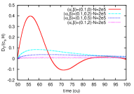
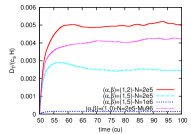
Figure 15: Time evolution of the diffusion coefficient. $D_{\mathrm{\scriptstyle{T}}}/(c_{\mathrm{s}}H)$ computed at $R=2$. Left: low artificial viscosity simulations (S1, S2, S3, S4). Right: higher artificial viscosity (S7, S8, S24 with MG83 implementation and S17 with Mu96 implementation). Note the different vertical scales.

The asymptotic values of the diffusion coefficient for each performed simulation are displayed in Fig. 16.

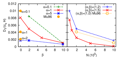
Figure 16: Results for $D_{\mathrm{\scriptstyle{T}}}$. Left: effect of artificial viscosity, right: effect of resolution.

Effect of artificial viscosity. The left panel of Fig. 16 shows that the coefficient decreases with increasing $\alpha$ and $\beta$ (except simulations from S1 to S3 which present a diffusion coefficient without a clear trend, due to the higher noise level) and in the Mu96 case (the artificial viscosity switch on approaching/receding particles is off, resulting in more viscous discs). This trend is due to a reduction of the noise that allows the onset of meridional circulation, which forces the fluid to be more localised in the vertical direction.

Effect of resolution. From the right panel of Fig.16 we observe that the diffusion coefficient decreases with increasing resolution. The reason of this behaviour is the same that explains the qualitatively similar trend we have observed in Sect. 4.3.1 for the central mass accretion rate. In this case, the PDF of the vertical velocity $v_{z}$ is broader in low resolution simulations with respect to more resolved simulations. Therefore, larger vertical velocity are possible in less resolved discs with resulting higher values (see Eq. 21) of the diffusion coefficient. The curve shows a converging trend, however convergence is not yet reached at one million particles. As for the central mass accretion rate and for the effective viscosity fit, convergence requires more resolution because the diffusion coefficient is computed from a smaller subset of particles than in the case of the radial velocity maps and the mass accretion rate profiles, where an average on the azimuthal component is taken.

We conclude that the diffusive mechanism is correctly represented by intermediate/large AV parameters $(\alpha,\beta)$: more viscous discs are less diffusive, due to the onset of meridional circulation and the decrease of $\alpha_{\mathrm{\scriptstyle{RS}}}$. In addition, for a given $(\alpha,\beta)$ combination, less resolved discs are more diffusive: such numerical dependence is of the same type as the dependence of the central mass accretion rate and of the effective viscosity on the resolution of the simulation (see Sect. 4.3.1.)

5.3 Mach number of velocity fluctuations

The azimuthally averaged Mach number of the modulus of velocity fluctuations is displayed in the $R$–$z$ plane in the left panel of Fig. 17 for simulation S23, as an example. The right panel shows the corresponding radial profile for each velocity component, vertically and azimuthally averaged. All simulations show qualitatively similar structures and profiles.

Effect of artificial viscosity. The average value of $\mathrm{Ma}_{\mathrm{f}}$ in the radial range $R\in[1,2.5]$ is displayed in Fig. 18. From the left panel of the figure, we see that, except for simulation S1, whose fluctuations are close to the sonic regime, all simulations show subsonic fluctuations with Mach number significantly smaller than unity. We observe a decrease of the average Mach number with larger AV parameters. For relatively high $\alpha$ and $\beta$, at each given radius the Mach number increases from a minimum value in the midplane ($\mathrm{Ma}_{\mathrm{f}}\approx 0.1$) to a maximum value in the surface layers ($\mathrm{Ma}_{\mathrm{f}}\approx 0.2$), as displayed by the left panel of Fig. 17. This behaviour is qualitatively in agreement with what is found in MHD simulations (e.g. Fromang & Nelson, 2006; Flock et al., 2011), however we observe smaller values. A global maximum $\mathrm{Ma}_{\mathrm{f}}\approx 0.4$ is reached in the inner region, where $v_{R}<0$ and the two accreting layers meet. In addition, two layers with locally higher fluctuations with $\mathrm{Ma}_{\mathrm{f}}\approx 0.2$ are also present at the interface between the surface accreting layers and the midplane outwards flow.

Effect of resolution. Similarly, as a consequence of noise reduction, higher resolution leads to a decrease both of the Mach number and of the extension of the surface layers where it reaches the local maximum for a given radial position (with the same qualitative behaviour of the accreting layers in the $v_{R}$ maps, see Figs. 3 and 4), as expected. We have found a convergence of the vertically and azimuthally averaged Mach number for a number of particles $N\approx 5\cdot 10^{5}$ (see right panel of Fig.18), in agreement with the value found for radial velocity maps (which are connected to radial velocity fluctuations and therefore to the radial part of the Mach number).

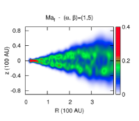
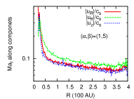
Figure 17: Mach number of velocity fluctuations. Left: azimuthal average in the $R$–$z$ plane, right: radial profile of the vertical and azimuthal average for each velocity component, in simulation S23.

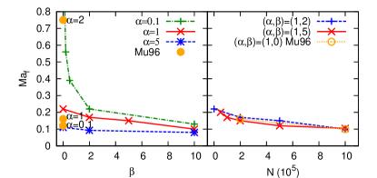
Figure 18: Results for $\mathrm{Ma}_{\mathrm{f}}$. Effect of changing the AV parameters and the AV switch (left panel) and resolution (right panel).

Fluctuations tends to be dominant in the regions of the disc where accreting and decreting flows meet: the cone-like regions between the accreting surface layers and the decreting midplane layer, and the region around the inner disc edge.

6 The structure of SPH fluctuations

6.1 Anisotropy of velocity fluctuations

We recall that when $\delta_{R}=2$ the system is totally radially anisotropic, while for negative values the system is dominated by anisotropy in different directions. The same holds for the azimuthal and vertical components. The kind of anisotropy of the disc is displayed in Fig. 19 for simulations with changing $\alpha$ and $\beta$. We observe that none of the simulated discs is totally anisotropic in one particular direction, but there is always a component that dominates the other two.

Effect of artificial viscosity. Discs with smaller AV parameters are dominated by radial anisotropy. For example, in the case of simulation S1 with ($\alpha$,$\beta$)=(0.1,0), we see from Fig. 19 that $\delta_{R}\approx 1.4$, $\delta_{\theta}<-1$ and $\delta_{z}<-1$, it follows that $\delta_{R}$ is significantly larger both than $\delta_{\theta}$ and than $\delta_{z}$. When $\alpha$ and/or $\beta$ are increased, $\delta_{R}$ decreases and becomes negative while $\delta_{\theta}$ increases. The vertical anisotropy is always negligible with respect to the radial or azimuthal anisotropy (it is always negative in all performed simulations, as shown by the right panel in Fig. 19).

Effect of resolution More resolved simulations are slightly more azimuthally anisotropic. As for some of the previously considered quantities, we observe that the components of the anisotropy vector, averaged in the vertical, azimuthal and in the usual radial range $R\in[1,2.5]$, converge at $N\approx 5\cdot 10^{5}$ (not shown), for the same reason already outlined several times.

We note that radial anisotropy has been observed in MHD discs (see e.g. Fromang & Papaloizou, 2006; Fromang & Nelson, 2006) where the mechanism of meridional circulation is absent. Here we observe radially dominated discs only for low AV parameters, for which meridional circulation is also absent.

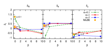
Figure 19: Results for $\vec{\delta}$, the anisotropy vector of velocity fluctuations. Effect of changing the AV parameters and the AV switch (MG83 and Mu96), values are averaged vertically, azimuthally and in the radial domain $[1,2.5]$. Note that values of the azimuthal and vertical anisotropy (middle and right panel) for $\beta=0$ become highly negative, they fall outside of the displayed area.

6.2 Power spectrum

For each simulation we have computed the power spectrum of velocity fluctuations in a ring located at different radii from the central star and at several altitudes, as explained in Sect. 3.2. As an example, in Figs. 20 and 21 we present compensated spectra (divided by the Kolmogorov slope of $-5/3$, for easy comparison) evaluated at the midplane location $(R,z)$=$(2,0)$ Different locations in the discs are considered later on.

Since we are dealing with an anisotropic system, we look at the one-dimensional power spectrum in the three directions: radial, azimuthal and vertical, which are given respectively in the first, second and third column of each row of the two figures.

At least three regions can be identified in the power spectra extracted from simulations. These regions are defined by two wavenumbers: $k_{1}<k_{2}$. The smallest scale corresponds to the resolution limit of the simulation that is given by the smoothing length at the considered position $h(R,z)$ (since the discs are axisymmetric there is not dependence on $\theta$) and defines the largest wavenumber $k_{2}$ (for each curve, this is marked by a circle in the plots). The region beyond $k_{2}$ corresponds to length scales inside the smoothing length, which are below the resolution. Therefore, the resolved region of the spectrum is to the left of the circle. The other scale marks the boundary between regions of the spectrum described by power laws $P(k)=P_{0}k^{a}$ with a different slope: for $k<k_{1}$ the slope $a_{1}$ is close to zero, for $k_{1}<k<k_{2}$ the slope is called $a_{2}$ and is always negative.

In the case of isotropic turbulence one could identify $k_{1}$ with the ‘forcing scale’ and the region between $k_{1}$ and $k_{2}$ with the ‘inertial range’. However, in the present anisotropic case, it is not possible to find a direct link between $k_{1}$ and the forcing scale in the disc because of the aliasing phenomenon present in one-dimensional spectra of turbulent shear-stress fluids (see e.g. Pope, 2000), since the power corresponding to wavenumber $k_{1}$ also contains contribution from larger wavenumbers.

In the following we focus on the qualitative evolution of the power spectrum with changing artificial viscosity and resolution.

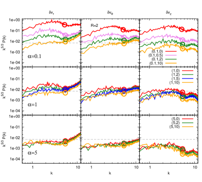
Figure 20: Compensated power spectrum $k^{5/3}P(k)$ of the velocity field. Effect of changing $\alpha$ and $\beta$. The three columns from left to right refer respectively to radial, azimuthal and vertical velocity components. The power spectrum is computed along a ring located at $R=2$ and $z=0$. The circle on each curve marks the wavenumber corresponding to the scale of the smoothing length. The number of particles is $N=2\cdot 10^{5}$.

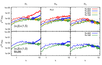
Figure 21: Compensated power spectrum of the velocity field. Effect of changing changing the AV switch and the resolution. The circle on each curve marks the wavenumber corresponding to the scale of the smoothing length.

Effect of artificial viscosity. What is interesting is the dependence of the shape of the power spectrum on the AV parameters. Simulations with $\alpha\lesssim 1$ and $\beta\lesssim 2$ show a positive slope of the compensated spectra with a decrease just before the resolution scale ($k\lesssim k_{2}$), which mimics the decay corresponding to the dissipation scale. In this case a cascade is not clearly identified in any of the three directions. An example is given by simulation S1 with ($\alpha$,$\beta$)=(0.1,0) in the top row of Fig. 20.

For higher AV parameters the behaviour of the power spectrum depends on the component of the velocity fluctuations, confirming that we are dealing with an anisotropic system also at intermediate scales. In particular, for radial velocity fluctuations in the case of $\alpha>1$ and $\beta>2$ (e.g. middle and bottom left panels of Fig. 20) and for the azimuthal component when $\alpha\approx 5$ and $\beta>2$ (bottom central panel of Fig. 20), a progressively more extended flat region (indicating a power spectrum with a slope close to the Kolmogorov value) is visible between the positive slope region on the left and the decay immediately before the resolution scale on the right. The other azimuthal spectra show a positive slope (e.g. top and middle central panels), indicating a sub-Kolmogorov slope. Concerning the vertical component of the velocity, flat regions start to appear for values of $\alpha$ close to 1, just above the resolution limit. However, they are less extended than in the case of the other two components. For higher $\alpha$, we observe that larger $\beta$ leads to a steeper slope.

In correspondence to the onset of meridional circulation, we observe the appearance of an approximately flat region in the compensated spectra for all velocity components and at the smallest resolved scales. This result suggests that the system is more isotropic at the small scales above the resolution limit.

Effect of resolution In agreement with previous analyses, we observe a convergence of the power spectrum of velocity fluctuations when a number of particles $N\approx 5\cdot 10^{5}$ is used. In addition, higher resolution discs are characterised by a cascade that is globally more extended in the wavenumber space than in lower resolution discs because they resolve smaller length scales, corresponding to larger wavenumbers. The resolution scale $k_{2}$ therefore shifts towards larger values (see Fig. 21).

In numerical simulations of turbulence a pile-up of energy (positive slope of the spectrum) is often observed in the high wavenumber region of the power spectrum (corresponding to the pre-dissipative region, close to grid resolution) and is probably due to numerical dissipation. We observe a similar feature only in the power spectrum of radial velocity fluctuations in intermediate and large viscosity discs (see left panels in Fig. 20 and 21). The pile-up is reduced by increasing resolution (see left panels in the top two rows in Fig. 21), supporting the numerical origin of the phenomenon.

Simulations are observed to converge towards a power spectrum with a cascade close to the Kolmogorov one for the radial and azimuthal components. The system reflects its anisotropy in a cascade that is always more extended for radial fluctuations and very short for vertical velocity fluctuations. Such a particular feature of the cascade is due to the different physical scales present in the disc, which is more radially than vertically extended (the disc is thin).

Changing location in the disc. The trends of the power spectrum observed with changing artificial viscosity and resolution are qualitatively similar at different radial locations in the disc (not shown).

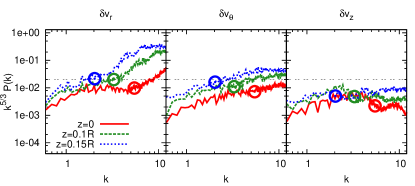
Figure 22: Compensated power spectrum of the velocity field. Effect of changing the location inside the disc. Power spectrum computed along a ring located at $R=2$ and at three different heights above the midplane for simulation S8 with $(\alpha,\beta)=(1,5)$.

In Fig. 22 spectra at different heights above the midplane are compared for each of the three velocity components in the case of simulation S8 where $(\alpha,\beta)=(1,5)$: moving away from the midplane, the slope of the cascade becomes slightly smaller and the cascade disappears due to decreasing resolution. In fact, at higher altitude the gas density is lower, implying a larger smoothing length (i.e. worse resolution). The wavenumber associated to the larger smoothing length is smaller and therefore it is closer to the wavenumber of the ‘forcing scale’, shortening the cascade.

We conclude that the power spectrum preserves its properties throughout the vertical and radial extension of the disc in the resolved regions of the wavenumber space.

6.3 Intermittency

In order to determine if intermittency is present in the simulations we analysed the PDF of the density and of the acceleration in the azimuthal direction (the direction of the shear) and the $3^{\mathrm{\scriptstyle{rd}}}$ and $4^{\mathrm{\scriptstyle{th}}}$ order moment of the PDF of several quantities.

6.3.1 Density and azimuthal acceleration PDF

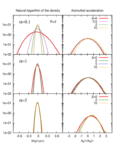
Figure 23: Probability distribution functions. Effect of AV parameters. Left: natural logarithm of the density. Right: acceleration. PDFs are computed at the midplane and at distance $R=2$ from the central star. The density PDF is compared to a log-normal distribution (dashed line) in the top left panel.

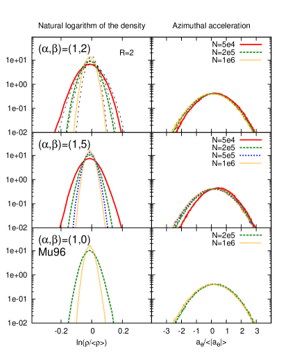
Figure 24: Probability distribution functions. Effect of resolution. Left: natural logarithm of the density. Right: acceleration. PDFs are computed at the midplane and at distance $R=2$ from the central star. The density PDF is compared to a log-normal distribution (dashed line) in the top left panel.

Effect of artificial viscosity. The effects of the AV parameters on the shape of the PDF of the natural logarithm of the density are shown in the left panel of Fig. 23. The distribution of ln$(\rho/\langle\rho\rangle)$ is described by a Gaussian distribution. It follows that the density is characterised by a log-normal distribution, as observed in simulations of supersonic compressible turbulence (see e.g. Price & Federrath, 2010, and Sect. 3.2.2).

However, in our simulations the standard deviation of the density logarithm $\sigma_{p}$, which controls the width of the distribution, is much smaller, since we are dealing with subsonic physical fluctuations (as shown in Sect. 5.3, Fig. 17 and Eq. 26). In addition, we observe that larger values of $\alpha$ and/or $\beta$ lead to a narrower distribution. This behaviour is explained by the same reason: the Mach number of physical fluctuations decreases and leads to a smaller $\sigma_{p}$, which in turn produces a PDF close to a Gaussian distribution and gives values of the skewness and kurtosis close to Gaussian values (as we will show in Sect. 6.3.2 and as expected from Eq. 27). The effect of changing $\beta$ for a given $\alpha$ is smaller than that of changing $\alpha$ for a given $\beta$, due to the fact that $\beta$ controls the second order term in the MG83 artificial viscosity.

It should be noted here that even for high $\alpha$ and/or $\beta$, although the effective viscosity becomes larger, the Reynolds stress is always non zero and still contributes to it. Therefore physical fluctuations are present and the disc is not laminar. For example, in our discs when $\alpha\approx 5$ the effective viscosity increases to $\alpha_{\mathrm{\scriptstyle{2D}}}\approx 0.1$ and the Reynolds stress amounts to $\alpha_{\mathrm{\scriptstyle{RS}}}\approx 10^{-3}$, with a corresponding turbulent Reynolds number $\mathrm{Re}_{\mathrm{\scriptstyle{T}}}\approx 10^{4}$, see Sect. 5.1 and Figs. 12 and 13. If the disc were laminar, one would not expect a distribution of densities but a single value, and therefore a delta function.

In the right column of Fig. 23 we show the PDF of the acceleration in the azimuthal direction since it presents an interesting feature: the distribution shifts towards higher values when both $\alpha$ and $\beta$ are increased. This is an effect of the onset of meridional circulation in discs with high enough artificial viscosity. In fact, the presence of meridional circulation imposes a net positive radial velocity (outward flow) to the gas around the midplane that, combined with the disc rotation, implies a spiral-like flow. The acceleration is thus characterised by a positive average azimuthal component (in contrast to a pure circular flow where the acceleration is only radial). The peak location moves towards the value $a_{\theta}/\langle|a_{\theta}|\rangle$=1 for larger AV parameters, however it does not reach unity even for the larger AV combination considered here ($\alpha,\beta$)=(5,10) since a fraction of the particles still presents a small but negative azimuthal component of the acceleration. Finally, the PDF of the radial and vertical components of the acceleration (not shown here) present the standard features of a pure circular flow: both of them have a symmetric shape with the peak located around the non-zero Keplerian value or around zero, respectively.

Effect of resolution. The effect of resolution is shown in Figure 24. For all the combinations of AV parameters, more resolved discs are characterised by a narrower density PDF (left column), due to the reduction in the numerical noise. The azimuthal acceleration PDF (right column) is only slightly affected, with the peak shifted towards smaller acceleration for higher resolution, due to a correspondingly lower strength of meridional circulation (see Sect. 4.2). As already found in previous analysed quantities, a number of particles as large as $N\approx 5\cdot 10^{5}$ guarantees a good degree of convergence.

In conclusion, the PDFs of density fluctuations reproduce those expected for non intermittent subsonic turbulent flows, confirming that the discs are not laminar.

6.3.2 Higher order moments: S and K

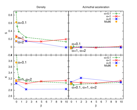
Figure 25: Higher order moments. Skewness (top) and kurtosis (bottom) of density distribution (left) and azimuthal acceleration distribution (right).

Effect of artificial viscosity. For a given $\alpha$, larger values of $\beta$ result in values of the skewness of the density PDF closer to the Gaussian value $S=0$ (top left plot in Fig. 25). The same effect is observed when $\beta$ is kept constant and $\alpha$ increased. All other quantities show Gaussian values independently of the AV parameter used, an example is given by the azimuthal component of the acceleration (top right plot in Fig. 25). Deviations of the kurtosis from the Gaussian value $K=3$ are qualitatively the same as for the skewness.

The simulations with the Mu96 artificial viscosity show systematically lower values of $S$ and $K$ with respect to simulations with the MG83 artificial viscosity and with the same $\alpha$ and $\beta=0$. The reason is that for the same $\alpha$, Mu96 discs are more viscous than MG83 discs since artificial viscosity is applied to all particles in contrast to the MG83 case. This trend is in agreement with that observed in MG83 simulations with changing AV parameters: more viscous discs present lower $S$ and $K$.

Effect of resolution. The values of S and K only show small fluctuations when the resolution is increased (not shown), suggesting that convergence for these global quantities is present even for a number of particle as low as $N\approx 2\cdot 10^{5}$.

In conclusion, no significant deviation from a Gaussian distribution is observed: intermittency is not present. This result agrees with the intermediate turbulent Reynolds number $\textrm{Re}_{\mathrm{\scriptstyle{T}}}$ proper to the present simulations (see Sect. 5.1). In fact intermittency is usually observed in very high Reynolds number flows (e.g. Frisch, 1996).

7 Discussion and conclusion

We have presented the characterisation of the global flow and of the statistical properties of the fluctuations in the velocity and density field of the gas in SPH disc models, which are gaseous discs simulated by means of the SPH method.

An essential tool for most of our results is the new method we have introduced for the determination of the effective viscosity of three dimensional axisymmetric discs. It consists in fitting the analytic expression for the radial velocity derived from two dimensional models (see e.g. TL02, ), depending both on $R$ and $z$, to the vertical velocity profile extracted from the simulation at different radial positions in the disc.

We have focused on the effects of changing the number of particles $N$ and the values of the two AV parameters $\alpha$ and $\beta$. The relevant results are summarised in the following points:

1. We have confirmed and quantified the numerical role of the number of particles $N$, which contributes to the numerical component of the SPH fluctuations (see its definition in Sect. 1). In fact, for all studied quantities, an increase in the resolution of the simulation (increase in the number of particles) has the standard numerical role of convergence towards the physical solution, and also leads to a more extended cascade in the power spectrum of velocity fluctuations (smaller scales and therefore higher wavenumbers are resolved).

2. More significantly, we have found that the artificial viscosity (through the two AV parameters $\alpha$ and $\beta$) contributes both to the numerical and to the physical component of the SPH fluctuations, in contrast to the behaviour of $N$.

There exists a relationship between artificial viscosity and the following three quantities: (a) physical fluctuations, quantified by $\alpha_{\mathrm{\scriptstyle{RS}}}$, (b) the effective viscosity of the disc, quantified by $\alpha_{\mathrm{\scriptstyle{2D}}}$ and (c) the numerical noise. In the hypothesis of an ideal noise-free numerical scheme, we expect that at low $(\alpha,\beta)$ the effective viscosity is due to turbulent viscosity, directly produced by physical fluctuations. At intermediate $(\alpha,\beta)$ the effective viscosity has a contribution not only from physical fluctuations but also from the AV term, which reproduces the effects of turbulence without directly modeling eddies and vortices in the spirit of the $\alpha_{\mathrm{\scriptstyle{SS}}}$-disc model. Finally, in the high $(\alpha,\beta)$ range, physical fluctuations are negligible and the effective viscosity is dominated by the AV term. However, numerical schemes are affected by numerical noise, which masks physical fluctuations.

In our case, noise is related to the AV parameters: only for $(\alpha,\beta)$ above a threshold is the noise reduced enough to allow physical fluctuations to emerge. We have identified the threshold at $(\alpha,\beta)\approx$ (1,2). In fact, in the discs simulated above this threshold, we have observed a sharp transition both of the global and of the local behaviour.

• Concerning the global behaviour, we have found that with increasing artificial viscosity the global flow of the gaseous disc evolves from a chaotic radial velocity structure to a more ordered meridional circulation pattern characterised by larger accretion rates and with the Reynolds number $\textrm{Re}_{\mathrm{\scriptstyle{eff}}}$, associated to the estimated effective viscosity $\alpha_{\mathrm{\scriptstyle{2D}}}$, below the turbulent limit for all simulations (however we observe that some of the high resolution simulations are approaching it).

• Concerning the local behaviour, we observe that, in parallel to the onset of meridional circulation, the average Reynolds stress switches abruptly from positive to negative values and converges to a value that contributes at the 10 per cent level to the effective viscosity ($\alpha_{\mathrm{\scriptstyle{RS}}}\approx 0.1\alpha_{\mathrm{\scriptstyle{2D}}}$), with an associated turbulent Reynolds number $\textrm{Re}_{\mathrm{\scriptstyle{T}}}$ around the turbulent limit. In particular, we have found that with increasing artificial viscosity, physical fluctuations have the following properties:

  • velocity fluctuations become more and more subsonic and shift from radial to azimuthal anisotropy;

  • a cascade appears in the power spectrum of velocity fluctuations, which tends towards a Kolmogorov-like spectrum, particularly for the radial component;

  • turbulent diffusion appears at the same time as the cascade and then the diffusion coefficient tends to decrease. Diffusion tends to be damped by the onset of meridional circulation;

  • the presence of meridional circulation leads to a shift of the peak of the azimuthal acceleration PDF;

  • none of the studied SPH disc models presents fluctuations characterised by intermittency.

With these results we can give a first answer to the question raised in the Introduction: can SPH disc models correctly reproduce both the observed properties of PPD and the expected effect of turbulence?

In the case of SPH disc models with the MG83 artificial viscosity we have found that for AV parameters above a threshold that approximately corresponds to the standard values ($\alpha\approx 1$ and $\beta\approx 2$), the effective viscosity mainly represents viscosity due to turbulence (of unknown origin) in the spirit of the SS73 $\alpha$-discs where intermediate and large scale turbulent eddies and vortices are not resolved. However, at the smallest resolved scales, fluctuations with properties similar to those present in turbulent flows have been identified. A meridional circulation pattern and turbulent-like fluctuations coexist in SPH disc models. The former shapes the global scale of the flow, reproducing the observed mass accretion rate onto the star while the latter is present locally at the smallest resolved scales and contributes to only 10 per cent of the effective viscosity of the disc. The resolved physical fluctuations reproduce the main effects expected in a turbulent 3D disc. In fact, the simulated discs are characterised by: a subsonic fluctuating velocity field presenting a turbulent-like diffusion and a small Kolmogorov-like cascade in the power spectrum of velocity fluctuations at the smallest resolved scales (see e.g. simulations S7 and S8). These simulations present values of the Reynolds stress and of the diffusion coefficient that are very close to those observed in MHD accretion discs (where the source of turbulence is the MRI). For values of $\alpha$ and $\beta$ below the threshold, the numerical noise dominates and masks physical fluctuations, these models should be avoided.

A direct detection of turbulent eddies would require a reduction of the AV term in order to increase the contribution of the Reynolds stress. However, we have shown that for the two AV implementations considered here the numerical noise dominates and impedes the growth of eddies in the velocity field when the levels of AV are below the threshold: in such cases the positive effects of the AV terms (particularly of the $\beta$ term) in correctly describing SPH particles trajectories and in avoiding particle interpenetration are missing. Therefore, in order to reach higher Reynolds numbers it is necessary both to reduce the effective viscosity of the disc without increasing the numerical noise and to increase the resolution. This is not possible with the two artificial viscosity implementation we are analysing in this work (since reducing the AV coefficients leads to an increase of the numerical noise). Recently developed artificial viscosity switches (e.g Morris & Monaghan, 1997; Cullen & Dehnen, 2010) could help in this direction. However, it is still not possible to simulate fluids at the high Reynolds numbers (Re${}_{\textrm{eff}}$ $\gg 10^{3}$) expected in astrophysical flows with the current tools and computer power.

We should stress that simulating very high Reynolds number discs would be necessary if one wanted to investigate the possibility of the existence of pure hydrodynamics turbulence in 3D accretion discs. (We remind the reader that 1D accretion discs are known to be stable with respect to hydrodynamics instabilities due to the Rayleigh criterion, see e.g. Armitage 2007.) However, for our purpose of reproducing the effects of turbulence produced by an unknown source, the effective viscosity combined with a low and possibly intermediate Reynols stress is enough. In fact, these models represent a starting point for the study of dust dynamics, which is affected by physical fluctuations at small scales and meridional circulation at large scales.

In conclusion, in SPH disc models, which a priori include only the ingredients of star gravity and physical-like-viscosity, we have found that the artificial viscosity term, in addition to modeling a physical-like bulk and shear viscosity, can also play the role of an implicit turbulence model. In our SPH disc models, where we do not add any initial turbulent velocity field, the implicit turbulence model sustains and organises the random fluctuations present in the initial conditions of the disc. This result is in agreement with recent indications that a turbulence model is implicitly present in the SPH scheme used to simulate homogeneous and isotropic turbulence with periodic boundary conditions (see e.g. Shi et al., 2012; Monaghan, 2011; Ellero et al., 2010). Here we have analysed the more complex case of systems without boundary conditions and where anisotropic turbulence is expected.

The effects of the density and sound speed profiles on the global and statistical properties of the gas as well as those of the initial set up, of different SPH kernels and of different artificial viscosity implementations will be addressed in more detail in a future work.

Appendix A Diagnostic details

A.1 The turbulent viscosity coefficient $\nu_{\mathrm{\scriptstyle{T}}}$

From the turbulent viscosity hypothesis (Pope, 2000), the Reynolds stresses are written in Cartesian coordinates as follows:

$$\langle u_{i}u_{j}\rangle=-2\nu_{\mathrm{\scriptstyle{T}}}\dot{\varepsilon}_{ij}-\frac{2}{3}k\delta_{ij},$$ (28)

where $\dot{\varepsilon}_{ij}$ is the rate of strain:

$$\dot{\varepsilon}_{ij}=\frac{1}{2}\left(\frac{\partial\langle v_{i}\rangle}{\partial x_{j}}+\frac{\partial\langle v_{j}\rangle}{\partial x_{i}}\right)$$ (29)

and $k$ the turbulent kinetic energy:

$$k=\frac{1}{2}\langle u_{i}u_{i}\rangle.$$ (30)

In classical accretion disc theory, only shear viscosity is relevant. Therefore the only non-vanishing component of the stress tensor is the $R\theta$ component (see e.g Lodato, 2008), which in cylindrical coordinates becomes:

$$\langle u_{R}u_{\theta}\rangle=-\nu_{\mathrm{\scriptstyle{T}}}\left[R\frac{\partial\left(\langle v_{\theta}\rangle/R\right)}{\partial R}+\frac{1}{R}\frac{\partial\langle v_{R}\rangle}{\partial\theta}\right].$$ (31)

Given the axisymmetry of the disc, the second term on the right hand side of Eq. 31 vanishes and the turbulent viscosity coefficient becomes:

$$\nu_{\mathrm{\scriptstyle{T}}}=-\frac{\langle u_{R}u_{\theta}\rangle}{R\left(\langle v_{\theta}\rangle/R\right)^{\prime}},$$ (32)

with $(\cdot)^{\prime}\equiv\partial/\partial R$.

A.2 The $\alpha_{\mathrm{\scriptstyle{RS}}}$ coefficient

The SS73 coefficient corresponding to the viscosity of Sect. A.1 is defined by the relation $\nu_{\mathrm{\scriptstyle{T}}}=\alpha_{\mathrm{\scriptstyle{RS}}}c_{\mathrm{s}}H$ that combined with Eq. 32 gives:

$$\alpha_{\mathrm{\scriptstyle{RS}}}=-\frac{\langle u_{R}u_{\theta}\rangle}{c_{\mathrm{s}}HR\left(\langle v_{\theta}\rangle/R\right)^{\prime}}$$ (33)

In the case of quasi-Keplerian discs we have: $\langle v_{\theta}\rangle$ $\approx$ $v_{\mathrm{k}}$ = $R\Omega_{\mathrm{k}}$, with $v_{\mathrm{k}}$ the Keplerian velocity and $\Omega_{\mathrm{k}}=\sqrt{GM}r^{-3/2}$ the corresponding angular velocity. For thin discs, the approximation $r\approx R$ holds, with $r$ the radial spherical component and $R$ the radial cylindrical component.

Remembering that the scale height of the disc is related to the sound speed and to the Keplerian angular velocity by $H=c_{\mathrm{s}}/\Omega_{\mathrm{k}}$, the $\alpha_{\mathrm{\scriptstyle{RS}}}$ coefficient takes the form:

$$\alpha_{\mathrm{\scriptstyle{RS}}}=-\frac{\langle u_{R}u_{\theta}\rangle}{R(\Omega_{\mathrm{k}})^{\prime}}\frac{\Omega_{\mathrm{k}}}{c_{\mathrm{s}}^{2}}=\frac{2}{3}\frac{\langle u_{R}u_{\theta}\rangle}{c_{\mathrm{s}}^{2}}.$$ (34)

A.3 The power spectrum, PDFs, $S$ and $K$

We consider a ring made of $N_{g}$ points and centred at the origin of the disc, with selected radius $R_{\mathrm{s}}$ and height $z_{s}$. The density and the smoothing length of each grid point are computed by means of an iterating procedure using the two coupled equations proper to the SPH scheme:

$$\rho_{a}=\sum_{b}m_{b}W_{ab}(r_{ab},h_{a});\qquad h_{a}=\eta\left(\frac{m_{a}}{\rho_{a}}\right)^{1/3},$$ (35)

where the subscript $a$ refers to the grid point and the subscript $b$ to its neighbours.

Once the smoothing length is known, the value of the desired quantities (e.g. velocity components for the power spectrum, density and azimuthal acceleration for the PDFs and higher order moments) at each grid point are computed by the SPH smoothing technique. Now the one dimensional list of values is known and used to compute the power spectrum of velocity components, the PDFs and the corresponding $S$ and $K$ coefficients.

This procedure is applied to each simulation snapshot, then values are averaged in time (for 15.9 orbits at 100 au). For $S$ and $K$ the standard deviation of the distribution of values in time has also been considered.

Appendix B Procedure for fitting the effective viscosity

The effective viscosity $\alpha_{\scriptstyle\textrm{2D}}$ in the disc is derived by fitting Eq. 15 to the data computed for a given snapshot of the simulation by means of the following three steps:

1. Computation of data from the selected simulation snapshot: radial profile $\Sigma(R)$ of the surface density, vertical profiles $\rho(z)$ and $v_{R}(z)$ of the volumetric density and radial velocity at radial position $R$.

2. Determination of the parameters present in Eq. 15. The surface density power law $p$ at the selected location $R$ is derived by fit of the surface density profile. The scale height $H$ of the disc at $R$ and $R_{0}$ is derived by fit of the relative vertical density profiles. Note that $q$ is constant, since simulations are locally isothermal, $R_{0}$ is the length unit and $c_{s_{0}}=H_{0}=H(R_{0})$ since $R_{0}=G=M=1$.

3. Determination of $\alpha_{\scriptstyle\textrm{2D}}$ by fit to the $v_{R}$ data.

All fits are performed by the general least square method, with $\chi^{2}$ function defined by:

$$\chi^{2}=\sum_{i=1}^{N}\left[\frac{y_{i}-f(x_{i},a)}{\sigma_{i}}\right]^{2},$$ (36)

where $(x_{i},y_{i})$ are the $N$ data points from simulations, $\sigma_{i}$ the associated errors and $f(x_{i},a)$ the function to be fitted, which depends on the parameter $a$.

References

- Andrews et al. (2009) Andrews S. M., Wilner D. J., Hughes A. M., Qi C., Dullemond C. P., 2009, ApJ, 700, 1502
- Armitage (2007) Armitage P. J., 2007, arXiv:0701485
- Balbus & Hawley (1991) Balbus S. A., Hawley J. F., 1991, ApJ, 376, 214
- Barrière-Fouchet et al. (2005) Barrière-Fouchet L., Gonzalez J.-F., Murray J. R., Humble R. J., Maddison S. T., 2005, A&A, 443, 185
- Bertin (2000) Bertin G., 2000, Dynamics of Galaxies
- Carballido et al. (2008) Carballido A., Stone J. M., Turner N. J., 2008, MNRAS, 386, 145
- Cullen & Dehnen (2010) Cullen L., Dehnen W., 2010, MNRAS, 408, 669
- Cuzzi et al. (1993) Cuzzi J. N., Dobrovolskis A. R., Champney J. M., 1993, Icarus, 106, 102
- Cuzzi et al. (2008) Cuzzi J. N., Hogan R. C., Shariff K., 2008, ApJ, 687, 1432
- Ellero et al. (2010) Ellero M., Español P., Adams N. A., 2010, Phys. Rev. E, 82, 046702
- Flock et al. (2012) Flock M., Dzyurkevich N., Klahr H., Turner N., Henning T., 2012, ApJ, 744, 144
- Flock et al. (2011) Flock M., Dzyurkevich N., Klahr H., Turner N. J., Henning T., 2011, ApJ, 735, 122
- Frisch (1996) Frisch U., 1996, Turbulence
- Fromang et al. (2011) Fromang S., Lyra W., Masset F., 2011, A&A, 534, A107
- Fromang & Nelson (2006) Fromang S., Nelson R. P., 2006, A&A, 457, 343
- Fromang & Nelson (2009) Fromang S., Nelson R. P., 2009, A&A, 496, 597
- Fromang & Papaloizou (2006) Fromang S., Papaloizou J., 2006, A&A, 452, 751
- Guilloteau et al. (2012) Guilloteau S., Dutrey A., Wakelam V., Hersant F., Semenov D., Chapillon E., Henning T., Piétu V., 2012, A&A, 548, A70
- Hartmann et al. (1998) Hartmann L., Calvet N., Gullbring E., D’Alessio P., 1998, ApJ, 495, 385
- Hughes et al. (2011) Hughes A. M., Wilner D. J., Andrews S. M., Qi C., Hogerheijde M. R., 2011, ApJ, 727, 85
- Jacquet (2013) Jacquet E., 2013, A&A, in press (arXiv:1301.5817)
- King et al. (2007) King A. R., Pringle J. E., Livio M., 2007, MNRAS, 376, 1740
- Klahr & Bodenheimer (2003) Klahr H. H., Bodenheimer P., 2003, ApJ, 582, 869
- Laibe et al. (2012) Laibe G., Gonzalez J.-F., Maddison S. T., 2012, A&A, 537, A61
- Lattanzio et al. (1985) Lattanzio J. C., Monaghan J. J., Pongracic H., Schwarz M. P., 1985, MNRAS, 215, 125
- Lodato (2008) Lodato G., 2008, New Astronomy Reviews, 52, 21
- Lodato & Price (2010) Lodato G., Price D. J., 2010, MNRAS, 405, 1212
- Lovelace et al. (1999) Lovelace R. V. E., Li H., Colgate S. A., Nelson A. F., 1999, ApJ, 513, 805
- Lynden-Bell & Pringle (1974) Lynden-Bell D., Pringle J. E., 1974, MNRAS, 168, 603
- Meglicki et al. (1993) Meglicki Z., Wickramasinghe D., Bicknell G. V., 1993, MNRAS, 264, 691
- Meru & Bate (2012) Meru F., Bate M. R., 2012, MNRAS, 427, 2022
- Monaghan (1992) Monaghan J. J., 1992, ARA&A, 30, 543
- Monaghan (2005) Monaghan J. J., 2005, Reports on Progress in Physics, 68, 1703
- Monaghan (2011) Monaghan J. J., 2011, European Journal of Mechanics - B/Fluids, 30, 360
- Monaghan & Gingold (1983) Monaghan J. J., Gingold R. A., 1983, Journal of Computational Physics, 52, 374
- Monaghan & Lattanzio (1985) Monaghan J. J., Lattanzio J. C., 1985, A&A, 149, 135
- Morris & Monaghan (1997) Morris J. P., Monaghan J. J., 1997, Journal of Computational Physics, 136, 41
- Murray (1996) Murray J. R., 1996, MNRAS, 279, 402
- Nelson et al. (2012) Nelson R. P., Gressel O., Umurhan O. M., 2012, ArXiv e-prints
- Pope (2000) Pope S. B., 2000, Turbulent Flows. Cambridge University Press
- Price (2007) Price D. J., 2007, PASA, 24, 159
- Price (2012) Price D. J., 2012, MNRAS, 420, L33
- Price & Federrath (2010) Price D. J., Federrath C., 2010, MNRAS, 406, 1659
- Pringle (1981) Pringle J. E., 1981, Annual review of astronomy and astrophysics, 19, 137
- Rice et al. (2011) Rice W. K. M., Armitage P. J., Mamatsashvili G. R., Lodato G., Clarke C. J., 2011, MNRAS, pp 1535–+
- Rice et al. (2005) Rice W. K. M., Lodato G., Armitage P. J., 2005, MNRAS, 364, L56
- Sargent et al. (2009) Sargent B. A., Forrest W. J., Tayrien C., McClure M. K., Watson D. M., Sloan G. C., Li A., Manoj P., Bohac C. J., Furlan E., Kim K. H., Green J. D., 2009, ApJS, 182, 477
- Schäfer (2005) Schäfer C., 2005, PhD thesis, Eberhard-Karls Universität Tübingen
- Shakura & Sunyaev (1973) Shakura N. I., Sunyaev R. A., 1973, in H. Bradt & R. Giacconi ed., X- and Gamma-Ray Astronomy Vol. 55 of IAU Symposium, Black Holes in Binary Systems: Observational Appearances. pp 155–+
- Shi et al. (2012) Shi Y., Ellero M., Adams N. A., 2012, Phys. Rev. E, 85, 036708
- Takeuchi & Lin (2002) Takeuchi T., Lin D. N. C. ., 2002, ApJ, 581, 1344
- Violeau & Issa (2007) Violeau D., Issa R., 2007, International Journal for Numerical Methods in Fluids, 53, 277