Universality of the momentum band density of periodic networks

Abstract

The momentum spectrum of a periodic network (quantum graph) has a band-gap structure. We investigate the relative density of the bands or, equivalently, the probability that a randomly chosen momentum belongs to the spectrum of the periodic network. We show that this probability exhibits universal properties. More precisely, the probability to be in the spectrum does not depend on the edge lengths (as long as they are generic) and is also invariant within some classes of graph topologies.

The spectrum of Schrödinger operator in periodic medium is calculated using the Floquet–Bloch procedure (Kittel, 1963): the periodic medium is replaced with its fundamental domain endowed with parameter-dependent quasi-periodic boundary conditions. The resulting parameter-dependent spectrum is called the dispersion relation, and the range of the dispersion relation is precisely the spectrum of the original structure. The spectrum has a band-gap structure and knowing the band location and sizes is of utmost importance in the theories of condensed matter and of dielectric and acoustic media (Yablonovitch, 1987; Zaanen et al., 1985; Figotin and Klein, 1998; Luo et al., 2003; Konoplev et al., 2010). Of particular recent interest is understanding the spectrum of quantum graphs (Berkolaiko and Kuchment, 2013; Gnutzmann and Smilansky, 2006), motivated by their application to solid state (Avron et al., 1994; Akkermans et al., 2000), photonic crystals (Kuchment and Kunyansky, 2002), carbon nano-structures (Kuchment and Post, 2007) as well as their use as models for quantum chaos, both in theoretical (Kottos and Smilansky, 1997; Berkolaiko et al., 2002; Gnutzmann and Altland, 2004; Gnutzmann et al., 2008, 2013; Joyner et al., 2013) and experimental (Hul et al., 2004, 2012) studies.

In the present Letter we explore the relative size of bands and gaps and discover a curious universality. To be more precise, we ask the following question: what is the probability $p_{s}$ that a randomly and uniformly chosen momentum belongs to the spectrum of the graph? For example, consider the $\mathbb{Z}^{1}$-periodic graphs of Fig. 1. How does $p_{\sigma}$ change if we change the lengths in the fundamental cell of the graph, from Fig. 1(b) to Fig. 1(c)? How does $p_{\sigma}$ change if we change the topological structure to Fig. 1(d) or 1(e)?

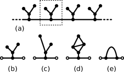
Figure 1: (a) An example of a $\mathbb{Z}^{1}$-periodic graph and (b) its fundamental cell; (c)-(e) are other examples of the fundamental cell.

Denote by $p_{\sigma}\left(K\right)$ the probability of a uniformly chosen momentum $k\in\left[0,K\right]$ to be in the spectrum and let $p_{\sigma}:=\lim_{K\rightarrow\infty}p_{\sigma}\left(K\right)$. We find that the probability $p_{\sigma}$ is well-defined and is independent of many features of the fundamental cell. In particular, all choices in Fig. 1(b) to (d) lead to the same value of $p_{\sigma}$ (assuming a generic choice of edge lengths). This is illustrated by a numerical simulation in Fig. 2. We will derive the limiting value analytically below. Note that the value of $p_{\sigma}$ for the cell in Fig. 1(e) turns out to be different from the others and will also be calculated.

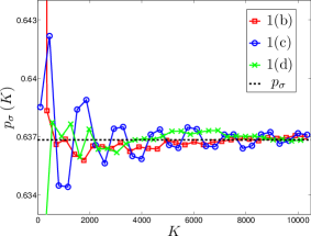
Figure 2: (color online) Numerical simulation of the convergence of $p_{\sigma}\left(K\right)$ is shown for the three periodic graphs from Fig. 1(b)-(d). The limiting value, $p_{\sigma}$, is shown as a dashed line. The graph lengths are normalized such that $K$ equals the average number of spectral bands.

Let us put the discussion onto a more formal footing. We consider a $\mathbb{Z}^{d}$-periodic network of quantum wires on which we are solving the spectral problem

$$-\frac{d^{2}\psi}{dx^{2}}=k^{2}\psi,$$ (1)

subject to the Kirchhoff–Neumann vertex conditions

$$\begin{cases}\psi(x)\text{ is continuous at }v,\\[5.0pt] \sum_{e\in\mathcal{E}_{v}}\frac{d\psi}{dx_{e}}(v)=0,\end{cases}$$ (2)

where the sum is over the edges $\mathcal{E}_{v}$ emanating from the vertex $v$ and the derivatives are taken into the edge. We denote by $\sigma$ the set of $k$ values for which there is a solution to (1)-(2); this is the momentum spectrum of the graph. Now, the definition of $p_{\sigma}$ can be formally written as

$$p_{\sigma}=\lim_{K\to\infty}p_{\sigma}\left(K\right)=\lim_{K\to\infty}\frac{1}{K}\Big{|}\sigma\cap[0,K]\Big{|}.$$ (3)

In this Letter we establish several properties of the probability $p_{\sigma}$. First of all, the above limit always exists. In addition, if there is at least one gap in the spectrum, there are infinitely many gaps and $p_{\sigma}<1$. Similarly, if there is at least one non-flat band, there are infinitely many and $p_{\sigma}>0$. Finally, and perhaps most strikingly, provided the lengths of edges in the fundamental set are generic, the value of $p_{\sigma}$ is independent of their precise value. We also find that the value of $p_{\sigma}$ is independent of some details of the cell’s topology.

Secular equation and dispersion relation.

In the Floquet–Bloch procedure for quantum graphs (see, e.g., (Berkolaiko and Kuchment, 2013)) we identify a set of $J$ generators of the lattice of periods and assign to each a quasi-momentum variable $\alpha_{j}$, $j=1,\ldots,J$. If the vertices $v_{+}$ and $v_{-}$ of the fundamental cell are identified by the action of the $j$-th generator, we impose the quasi-periodic conditions

$$\psi(v_{+})=e^{i\alpha_{j}}\psi(v_{-}),\quad\psi^{\prime}(v_{+})=-e^{i\alpha_{j}}\psi^{\prime}(v_{-}).$$ (4)

We remind the reader that we use the convention of always taking the derivatives into the edge, which explains the minus sign in conditions (4). For example, in the fundamental cell of Fig. 1(b) the empty circles denote the vertices connected through the condition of the above type. Identifying these periodically related vertices creates new cycles, $C_{j}$, $j=1,\ldots,J$, on the graph and the resulting problem is equivalent to a graph with magnetic fluxes $\alpha_{j}$ through the corresponding cycles. For example, the result of the Floquet–Bloch procedure for the fundamental cell in Fig. 1(d) is equivalent to the magnetic graph in Fig. 3(a). We denote by $E$ the number of edges of the resulting magnetic graph.

Expanding the solutions to (1) in the basis of $e^{\pm ikx}$ and applying the vertex conditions leads, after some linear algebra (see (Kottos and Smilansky, 1997)), to the secular equation

$$F(k;\vec{\alpha}):=\det\left(\mathbf{1}-\mathrm{e}^{i\left(\mathbf{A}+k\mathbf{L}\right)}\mathbf{S}\right)=0,$$ (5)

where all matrices act in the space of coefficients on directed edges; each edge gives rise to two directed edges of equal length, therefore all matrices have degree $2E$. The diagonal matrix $\mathbf{L}$ is the matrix of lengths of the directed edges. The diagonal matrix $\mathbf{A}$ contains the magnetic fluxes $\alpha_{j}$ that are put upon the edges created by vertex identifications. The magnetic fluxes change sign when reversing the direction of the corresponding edge. Finally, the unitary matrix $\mathbf{S}$ contains directed edge-to-edge scattering coefficients, which, for scattering at a Neumann-Kirchhoff vertex of degree $d$, is equal to $-1+2/d$ for back-scattering and $2/d$ for forward scattering. Most importantly, for our vertex conditions the matrix $\mathbf{S}$ is independent of $k$. See (10)–(11), which show these matrices for a specific graph.

Next we apply a clever trick originally due to Barra and Gaspard (Barra and Gaspard, 2000) (see also (Berkolaiko and Winn, 2010)): we introduce a new function $\Phi(\vec{\kappa};\vec{\alpha})$ such that

$$\Phi(\kappa_{1}=kl_{1},\ldots,\kappa_{E}=kl_{E};\vec{\alpha}):=F(k;\vec{\alpha}),$$ (6)

where $l_{1},\ldots,l_{E}$ are the graph edge lengths. A cursory look at equation (5) reveals that the variables $\kappa_{e}$, $e=1,\ldots,E$ need only be known modulo $2\pi$. For a fixed $\vec{\alpha}$, define $\Sigma_{\vec{\alpha}}$ to be the set of solutions of

$$\Phi(\vec{\kappa};\vec{\alpha})=0,$$ (7)

on the torus $\mathbb{T}_{E}:=\left[0,2\pi\right)^{E}$. Then the roots $k_{n}$ of the equation $F(k;\vec{\alpha})=0$ can be interpreted as the times ($k$ values) of piercing of the set $\Sigma_{\vec{\alpha}}$ by the flow

$$\vec{\kappa}\left(k\right)=k\cdot(l_{1},l_{2},\ldots,l_{E})\operatorname{mod}2\pi.$$ (8)

We now conclude that $k$ belongs to the spectrum, $\sigma$, of the periodic graph if the corresponding point $\vec{\kappa}(k)$ belongs to the set $\Sigma_{\vec{\alpha}}$ for some value of $\vec{\alpha}$ (which itself belongs to a $J$-dimensional torus). For future purposes we define

$$\Sigma=\bigcup_{\vec{\alpha}\in[0,2\pi)^{J}}\Sigma_{\vec{\alpha}}.$$ (9)

We will now compute the set $\Sigma$ in a simple but important example and then proceed to discuss how the questions about the band probability $p_{\sigma}$ can be related to the properties of the set $\Sigma$.

Loop with an edge.

We now compute the set $\Sigma$ for a graph which consists of a loop pierced by magnetic field with flux $\alpha$ and a single edge attached, see Fig. 3(b).

Figure 3: (a) A graph consisting of a loop pierced by a magnetic flux and a decoration (b) Similar graph, but with a single edge decoration

The numbering of the directed edges is given in Fig. 3(b). According to this numbering the matrices $\mathbf{A}$, $\mathbf{L}$ and $\mathbf{S}$ are given by

$$\mathbf{A}=\operatorname{diag}(\alpha,0,-\alpha,0),\quad\mathbf{L}=\operatorname{diag}(l_{1},l_{2},l_{1},l_{2}).$$ (10)

and

$$\mathbf{S}=\left(\begin{smallmatrix}\nicefrac{{2}}{{3}}&\nicefrac{{2}}{{3}}&-\nicefrac{{1}}{{3}}&0\\ 0&0&0&1\\ -\nicefrac{{1}}{{3}}&\nicefrac{{2}}{{3}}&\nicefrac{{2}}{{3}}&0\\ \nicefrac{{2}}{{3}}&-\nicefrac{{1}}{{3}}&\nicefrac{{2}}{{3}}&0\end{smallmatrix}\right)$$ (11)

The secular function $\Phi$ evaluates to (up to some non-zero factors)

$$\Phi=2\cos(\kappa_{2})\left(\cos(\kappa_{1})-\cos(\alpha)\right)\\ -\sin(\kappa_{1})\sin(\kappa_{2}).$$ (12)

The zero sets $\Sigma_{\alpha}$ for a range of values of the parameter $\alpha$ are shown on Fig. 4(a). Note that it is enough to consider the values $\alpha\in\left[0,\pi\right]$ as $\Sigma_{-\alpha}=\Sigma_{\alpha}$ (see (12)).

Figure 4: (color online) (a) The zero sets, $\Sigma_{\alpha},$ of $\Phi\left(\kappa_{1},\kappa_{2};\,\alpha\right)$ are shown for a range of values $\alpha\in\left[0,\pi\right]$ using a blue ($\alpha=0$) - red ($\alpha=\pi$) color scale. (b) The set $\Sigma=\bigcup_{\alpha\in[0,2\pi)}\Sigma_{\alpha}$ is shaded, its blue boundaries are the zeros of $\Phi\left(\cdot,\cdot;\,\alpha=0\right)$ and the red boundaries are the zeros of $\Phi\left(\cdot,\cdot;\,\alpha=\pi\right)$. A flow $\vec{\kappa}\left(k\right)=k\cdot\left(l_{1},l_{2}\right)$ on the torus is indicated. The bands of the spectrum $\sigma$ are the solid black segments of the flow line; the gaps are drawn in light gray.

Probability to be in the spectrum.

From the discussion above we conclude that the probability $p_{\sigma}$ for a random $k$ to be in the spectrum $\sigma$ is equal to the proportion of time the flow defined by (8) spends in the set $\Sigma$. Depending on the commensurability properties of the set of the edge lengths, $\left\{l_{e}\right\}_{e=1}^{E}$, the flow covers densely the entire torus or is restricted to a flat submanifold

$$L := \overline{\operatorname{span}\left(k\cdot(l_{1},l_{2},\ldots)\,\operatorname{mod}\mathbb{T}_{E}:k\in\mathbb{R}\right)}$$

$$= \left\{x\in\mathbb{R}^{E}:Mx=0\right\}\,\operatorname{mod}\mathbb{T}_{E},$$

where $M$ is a matrix with rational coefficients (it gives the rational dependencies in the length sequence $(l_{1},\ldots,l_{E})$). In the latter case, the flow is ergodic on the submanifold $L$. The probability $p_{\sigma}$ is therefore the relative volume

$$p_{\sigma}=\frac{\operatorname{vol}_{L}\left(L\cap\Sigma\right)}{\operatorname{vol}_{L}(L)},$$ (13)

where the subscript $L$ indicates that the volume should be taken in the appropriate dimension (equal to $E$ minus the rank of the matrix $M$). Formula (13) remains valid in the case of rationally independent lengths, when we simply take $L$ to be the entire torus. This immediately implies that the probability $p_{\sigma}$ remains the same as long as the edge lengths are rationally independent.

Returning to our example, we calculate $p_{\sigma}$ explicitly. Using symmetry we compute the area of $1/8$-th of the set $\Sigma$, the part in the lower left corner. It is bounded by the coordinate axes and the set $\Sigma_{\pi}$, which from (12) we re-parameterize as

$$\tan(\kappa_{2})=2\cot(\kappa_{1}/2).$$ (14)

Therefore the ratio in (13) evaluates to

$$p_{\sigma}=\frac{2}{\pi^{2}}\int_{0}^{\pi}\tan^{-1}\left(2\cot\left(\nicefrac{{\kappa}}{{2}}\right)\right)d\kappa\approx 0.64.$$ (15)

We can further prove that this universality of $p_{\sigma}$ extends to a certain class of decoration structures. These are the decorations that attach to the base line by means of a single edge, as in Fig. 1(a) to (d). Proving the universality is done by reducing the influence of the decoration on the secular equation to a single scattering reflection phase located at the degree one vertex of the graph in figure 3(b). The phase enter the matrix $\mathbf{S}$ as follows,

$$\mathbf{S}=\left(\begin{smallmatrix}\nicefrac{{2}}{{3}}&\nicefrac{{2}}{{3}}&-\nicefrac{{1}}{{3}}&0\\ 0&0&0&\Theta\left(\kappa_{3},\ldots,\kappa_{E}\right)\\ -\nicefrac{{1}}{{3}}&\nicefrac{{2}}{{3}}&\nicefrac{{2}}{{3}}&0\\ \nicefrac{{2}}{{3}}&-\nicefrac{{1}}{{3}}&\nicefrac{{2}}{{3}}&0\end{smallmatrix}\right).$$ (16)

While the precise form of the phase $\Theta\left(\kappa_{3},\ldots,\kappa_{E}\right)$ may be complicated, its effect on the function $\Phi$ gets averaged out by ergodicity. More precisely, we now assume that the rational relations (if any) defining the submanifold $L$ do not involve $\kappa_{1}$ and $\kappa_{2}$. In other words, the lengths of the edges $1$ and $2$ are rationally independent of each other and of the lengths of the decoration’s edges. We need not assume anything about the lengths of edges of the decoration.

One can now easily read from the determinant (see (5),(6)) that the function $\Phi$ has the form $\Phi\left(\kappa_{1},\kappa_{2},\ldots,\kappa_{E};\,\alpha\right)=\Phi\left(\kappa_{1},\kappa_{2}+\nicefrac{{1}}{{2}}\Theta\left(\kappa_{3},\ldots,\kappa_{E}\right);\,\alpha\right)$, where $\Phi\left(\cdot,\cdot;\,\alpha\right)$ in the RHS is as in (12). Introducing the change of variables

$$\hat{\kappa}_{2}=\kappa_{2}+\frac{1}{2}\Theta\left(\kappa_{3},\ldots,\kappa_{E}\right),$$ (17)

the integrals in (13) factorize. Namely, denote by $\mathbb{T}_{2}$ the torus with respect to $\kappa_{1}$ and $\hat{\kappa}_{2}$ and by $\mathbb{T}_{E-2}$ the torus with respect to the other variables. Note that the set $\Sigma$ depends only on the variables $\kappa_{1}$ and $\hat{\kappa}_{2}$ (and is cylindrical with respect to the other variables). The submanifold $L$, on the other hand, is cylindrical with respect to $\kappa_{1}$ and $\hat{\kappa}_{2}$. Therefore

$$p_{\sigma}=\frac{\operatorname{vol}_{\mathbb{T}_{2}}\left(\mathbb{T}_{2}\cap\Sigma\right)\operatorname{vol}_{\mathbb{T}_{E-2}}\left(\mathbb{T}_{E-2}\cap L\right)}{\operatorname{vol}_{\mathbb{T}_{2}}\left(\mathbb{T}_{2}\right)\operatorname{vol}_{\mathbb{T}_{E-2}}\left(\mathbb{T}_{E-2}\cap L\right)},$$ (18)

reducing to the expression in (13), where $L$ there is identified as $\mathbb{T}_{2}$ in (18). We thus proved that for all decorations of the type discussed above the probability to be in the spectrum is given by (15).

To give a final example of a different nature, for the fundamental cell depicted in Fig. 1(e), the secular equation can be shown to be equivalent to

$$\sin(\kappa_{1}+\kappa_{2}+\kappa_{3})-\frac{1}{2}\sin\kappa_{1}\sin\kappa_{2}\sin\kappa_{3}\\ =\sin\kappa_{1}+\cos\alpha(\sin\kappa_{2}+\sin\kappa_{3}),$$ (19)

and the corresponding value of $p_{\sigma}$ was calculated numerically to be $0.43$.

Conclusions.

The arguments presented above apply to all graphs and result in three general conclusions. First, given a $\mathbb{Z}^{d}$-periodic graph with an arbitrary fundamental cell, the probability $p_{\sigma}$ is independent of the specific edge lengths, as long as there are no rational dependencies between some of them. Even if such dependencies exist, an appropriate ergodicity argument shows that the limit (3) which defines $p_{\sigma}$ exists and its exact value depends on the nature of the edge lengths rational dependencies (as well as the graph’s topology). Secondly, we have shown that $p_{\sigma}$ is robust even within some topological modifications of the graph - attaching a prescribed class of decorations. Thirdly, if there exists at least one non-flat band (resp. gap) in the spectrum, it must arise from an open set on the torus which is a subset of $\Sigma$ (corresp. $\mathbb{T}\backslash\Sigma$). The ergodic flow on the torus will pass through this set infinitely many times, resulting in an infinite number of non-flat bands (resp. gaps) of comparable size. From equation (13) we can immediately conclude that $p_{\sigma}>0$ (resp. $p_{\sigma}<1$).

Our setup calls for comparison with periodic potentials on the line, in particular the singular potentials $\delta$ and $\delta^{\prime}$ (Albeverio et al., 2005). Note that we measure our band and gap sizes in terms of the momentum variable $k$, not energy (which scales as $k^{2}$). For smooth periodic potentials and $\delta$ potentials, the gaps sizes decrease as $k\to\infty$, while the band lengths converge to a constant, resulting in $p_{\sigma}=1$ (Weinstein and Keller, 1987; Exner and Gawlista, 1996). The $\delta^{\prime}$ potential has an opposite behavior, asymptotically equivalent to disconnecting the graph: the band lengths decrease and the gaps approach a constant size, resulting in $p_{\sigma}=0$ (Exner and Gawlista, 1996). Our results show that a typical non-trivial periodic graph has intermediate behavior with $0<p_{\sigma}<1$, as long as there is at least one gap and at least one band. One explanation of this phenomenon is that the graph of Fig. 1(a) (for example) can be viewed as a line with periodic $\delta$-potential (the so-called Kronig-Penney model) whose strength is momentum dependent. In such an analogue, the strength of the $\delta$-potential oscillates between infinity and zero, which in effect alternates between disconnecting the graph and having a perfect transmission, resulting with the intermediate values $0<p_{\sigma}<1$. We refer the reader to (Avron et al., 1994; Exner and Turek, 2010) for similar discussions.

One can also consider dressing the network with a bounded periodic potential and/or changing the vertex conditions from the ones we considered. This should not affect our results qualitatively, as the influence of a potential or vertex conditions decreases in the $k\to\infty$ limit. However, this case is technically more difficult since the $k$-dependence in equation (5) would become more involved. To overcome these difficulties, methods developed in (Bolte and Endres, 2009; Rueckriemen and Smilansky, 2012) might prove useful.

Some further interesting spectral questions are now within reach. One may obtain bounds on possible sizes of bands (gaps) and deduce the specific edge lengths for which they are attained. Furthermore, the gap opening mechanism, a well studied subject on its own right (Schenker and Aizenman, 2000; Kuchment, 2005), can be better understood by examining the sub-domains of the torus which do not intersect $\Sigma$. In addition, the topological meaning of $p_{\sigma}$ should be further investigated — does it relate to some other graph invariants or does it provide a brand new piece of information on the underlying graph?

Finally, we make another step forward by extending the discussion to eigenfunction properties. The number of zeros of an eigenfunction was recently found to be connected with the stability of the corresponding eigenvalue with respect to magnetic perturbations (Berkolaiko, 2011; Colin de Verdière, 2012; Berkolaiko and Weyand, 2012). The stability is described by the Morse index of the eigenvalue and most strikingly, this Morse index can be shown to be a well defined function on the torus, not depending on the direction of the flow (i.e., on graph edge lengths) (Band, 2012). This leads to new and exciting findings on the distribution of number of zeros of graph eigenfunctions (Band and Berkolaiko, 2013).

References

- Kittel (1963) C. Kittel, Quantum Theory of Solids (Wiley, New York, 1963).
- Yablonovitch (1987) E. Yablonovitch, Phys. Rev. Lett. 58, 2059 (1987).
- Zaanen et al. (1985) J. Zaanen, G. A. Sawatzky, and J. W. Allen, Phys. Rev. Lett. 55, 418 (1985).
- Figotin and Klein (1998) A. Figotin and A. Klein, SIAM Journal on Applied Mathematics 58, 1748 (1998).
- Luo et al. (2003) C. Luo, M. Ibanescu, S. Johnson, and J. Joannopoulos, Science 299, 368 (2003).
- Konoplev et al. (2010) I. V. Konoplev, L. Fisher, A. W. Cross, A. D. R. Phelps, K. Ronald, and C. W. Robertson, Appl. Phys. Lett. 96 (2010).
- Berkolaiko and Kuchment (2013) G. Berkolaiko and P. Kuchment, Introduction to quantum graphs, vol. 186 of Mathematical Surveys and Monographs (Amer. Math. Soc., Providence, RI, 2013), ISBN 978-0-8218-9211-4.
- Gnutzmann and Smilansky (2006) S. Gnutzmann and U. Smilansky, Advances in Physics 55, 527 (2006).
- Avron et al. (1994) J. E. Avron, P. Exner, and Y. Last, Phys. Rev. Lett. 72, 896 (1994).
- Akkermans et al. (2000) E. Akkermans, A. Comtet, J. Desbois, G. Montambaux, and C. Texier, Ann. Phys. 284, 10 (2000).
- Kuchment and Kunyansky (2002) P. Kuchment and L. Kunyansky, Adv. Comput. Math. 16, 263 (2002).
- Kuchment and Post (2007) P. Kuchment and O. Post, Comm. Math. Phys. 275, 805 (2007).
- Kottos and Smilansky (1997) T. Kottos and U. Smilansky, Phys. Rev. Lett. 79, 4794 (1997).
- Berkolaiko et al. (2002) G. Berkolaiko, H. Schanz, and R. S. Whitney, Phys. Rev. Lett. 88, 104101 (2002).
- Gnutzmann and Altland (2004) S. Gnutzmann and A. Altland, Phys. Rev. Lett. 93, 194101 (2004).
- Gnutzmann et al. (2008) S. Gnutzmann, J. P. Keating, and F. Piotet, Phys. Rev. Lett. 101, 264102 (2008).
- Gnutzmann et al. (2013) S. Gnutzmann, H. Schanz, and U. Smilansky, Phys. Rev. Lett. 110, 094101 (2013).
- Joyner et al. (2013) C. H. Joyner, S. Müller, and M. Sieber (2013), preprint arXiv:1302.2554 [math-ph].
- Hul et al. (2004) O. Hul, S. Bauch, P. Pakoński, N. Savytskyy, K. Życzkowski, and L. Sirko, Phys. Rev. E 69, 056205 (2004).
- Hul et al. (2012) O. Hul, M. Ławniczak, S. Bauch, A. Sawicki, M. Kuś, and L. Sirko, Phys. Rev. Lett. 109, 040402 (2012).
- Barra and Gaspard (2000) F. Barra and P. Gaspard, J. Statist. Phys. 101, 283 (2000).
- Berkolaiko and Winn (2010) G. Berkolaiko and B. Winn, Trans. Amer. Math. Soc. 362, 6261 (2010).
- Albeverio et al. (2005) S. Albeverio, F. Gesztesy, R. Høegh-Krohn, and H. Holden, Solvable models in quantum mechanics (AMS Chelsea Publishing, Providence, RI, 2005), 2nd ed., ISBN 0-8218-3624-2, with an appendix by Pavel Exner.
- Weinstein and Keller (1987) M. I. Weinstein and J. B. Keller, SIAM J. Appl. Math. 47, 941 (1987).
- Exner and Gawlista (1996) P. Exner and R. Gawlista, Phys. Rev. B 53, 7275 (1996).
- Exner and Turek (2010) P. Exner and O. Turek, Journal of Physics A: Mathematical and Theoretical 43, 474024 (2010).
- Bolte and Endres (2009) J. Bolte and S. Endres, Ann. Henri Poincaré 10, 189 (2009), ISSN 1424-0637.
- Rueckriemen and Smilansky (2012) R. Rueckriemen and U. Smilansky, J. Phys. A: Math. Theor. 45, 475205 (2012).
- Schenker and Aizenman (2000) J. H. Schenker and M. Aizenman, Lett. Math. Phys. 53, 253 (2000).
- Kuchment (2005) P. Kuchment, J. Phys. A 38, 4887 (2005).
- Berkolaiko (2011) G. Berkolaiko (2011), to appear in Anal. PDE; preprint arXiv:1110.5373 [math-ph].
- Colin de Verdière (2012) Y. Colin de Verdière (2012), to appear in Anal. PDE; preprint arXiv:1201.1110v2 [math-ph].
- Berkolaiko and Weyand (2012) G. Berkolaiko and T. Weyand (2012), to appear in Phil. Trans. Roy. Soc. A; preprint arXiv:1212.4475 [math-ph].
- Band (2012) R. Band (2012), to appear in Phil. Trans. Roy. Soc. A; preprint arXiv:1212.6710 [math-ph].
- Band and Berkolaiko (2013) R. Band and G. Berkolaiko (2013), in progress.