Spaces, Trees and Colors: The Algorithmic Landscape of Document Retrieval on Sequences

Abstract

Document retrieval is one of the best established information retrieval activities since the sixties, pervading all search engines. Its aim is to obtain, from a collection of text documents, those most relevant to a pattern query. Current technology is mostly oriented to “natural language” text collections, where inverted indexes are the preferred solution. As successful as this paradigm has been, it fails to properly handle various East Asian languages and other scenarios where the “natural language” assumptions do not hold. In this survey we cover the recent research in extending the document retrieval techniques to a broader class of sequence collections, which has applications in bioinformatics, data and Web mining, chemoinformatics, software engineering, multimedia information retrieval, and many other fields. We focus on the algorithmic aspects of the techniques, uncovering a rich world of relations between document retrieval challenges and fundamental problems on trees, strings, range queries, discrete geometry, and other areas.

Funded by Millennium Nucleus Information and Coordination in Networks ICM/FIC P10-024F.

1 Introduction

Retrieving useful information from huge masses of data is undoubtedly one of the most important activities enabled by computers in the Information Age, and text is the preferred format to represent and retrieve most of this data. Albeit images and videos have gained much importance on the Internet, even on those supports the searches are mostly carried out on text (e.g., Google finds images based on the text content around them in Web pages). The problem of finding the relevant information in large masses of text was already pressing in the sixties, where the basis of modern Information Retrieval techniques were laid out [Salton (1968)]. Nowadays, this has become one of the most important research topics in Computer Science [Croft et al. (2009), Büttcher et al. (2010), Baeza-Yates and Ribeiro-Neto (2011)].

Interestingly, besides a large degree of added complexity to permanently improve the search “quality” (i.e., how the returned information matches the need expressed by the query), the core of the approach has not changed much since Sal68’s time. One assumes that there is a collection of documents, each of which is a sequence of words. This collection is indexed, that is, preprocessed in some form. This index is able to answer queries, which are words, or sets of words, or sets of phrases (word sequences). A relevance formula is used to establish how relevant is each of the documents for the query. The task of the index is to return a set of documents most relevant to the query, according to the formula.

In the original vector space model [Salton (1968)], a set of distinguished words (called terms) was extracted from the documents. A weight $w(t,d)$ for term $t$ in document $d$ was defined using the assumption that a term appearing many times in a document was important in it. Thus a component of the weight was the term frequency, $\mathsf{tf}(t,d)$, which is the number of times $t$ appears in $d$. A second component was aimed to downplay the role of terms that appeared in many documents (such as articles and prepositions), as those do not really distinguish a document from others. The so-called inverse document frequency was defined as $\mathsf{idf}(t)=\lg(D/\mathsf{df}(t))$, where $D$ is the total number of documents and $\mathsf{df}(t)$ is the number of documents where $t$ appears. Then $w(t,d)=\mathsf{tf}(t,d)\times\mathsf{idf}(t)$ was the formula used in the famous “tf-idf” model. The query was a set of terms, $Q=\{q_{1},q_{2},\ldots,q_{m}\}$, and the relevance of a document $d$ for query $Q$ was $w(Q,d)=\sum_{i=1}^{m}w(q_{i},d)$. Then the system returned the top-$k$ documents for $Q$, that is, $k$ documents $d$ with the highest $w(Q,d)$ value. When computers became more powerful, the so-called full-text model took every word in the documents as a querieable term.

As said, this simple model has been sophisticated in recent years up to an amazing degree, including some features that are possible due to the social nature of the Internet: the intrinsic value of the documents, the links between documents, the fields where the words appear, the feedback and profile of the user, the behavior of other users that made similar queries, and so on. Yet, the core of the idea is still to find documents where the query terms appear many times.

The inverted index has always been the favorite structure to support these searches. The essence of this structure could not be simpler: given the vocabulary of all the querieable terms, the index stores a list of the documents $d$ where each such term $t$ appears, plus information to compute its weight $w(t,d)$ in each. Much research has been carried out to efficiently store and access inverted indexes [Witten et al. (1999), Büttcher et al. (2010), Baeza-Yates and Ribeiro-Neto (2011)], without changing its essential organization. All modern search engines use variants of inverted indexes.

Despite the immense success of this information retrieval model and implementation, it has a clear limitation: it strongly relies on the fact that the vocabulary of all the querieable terms has a manageable size. The empirical law proposed by Hea78 establishes that the vocabulary of a collection of size $n$ grows like $\Theta(n^{\beta})$ for some constant $0<\beta<1$, and it holds very accurately in many Western languages. The model, therefore, restricts the queries to be whole words, not parts of words. It is not even obvious how to deal with phrases. One could extend the concepts of $\mathsf{tf}$ and $\mathsf{idf}$ to phrases and parts of words, but this would be quite difficult to implement with an inverted index: in principle, it would have to store the list of documents where every conceivable text substring appears!

Such a limitation causes problems in highly synthetic languages such as Finnish, Hungarian, Japanese, German, and many others where long words are built from particles. But it is more striking in languages where word separators are absent from written text and can only be inferred by understanding its meaning: Chinese, Korean, Thai, Japanese (Kanji), Lao, Vietnamese, and many others. Indeed, “segmenting” those texts into words is considered a research problem belonging to the area of Natural Language Processing (NLP); see, e.g., RX12.

Out of resorting to expensive and heuristic NLP techniques, a solution for those cases is to treat the text as an uninterpreted sequence of symbols and allow queries to find any substring in those sequences. The problem, as said, is that inverted indexes cannot handle those queries. Instead, suffix trees [Weiner (1973), McCreight (1976), Apostolico (1985)] and suffix arrays [Gonnet et al. (1992), Manber and Myers (1993)], and their recent space-efficient versions [Navarro and Mäkinen (2007)] are data structures that efficiently solve the pattern matching problem, that is, they list all the positions in the sequences where a pattern appears as a substring. However, they are not easily modified to handle document retrieval problems, such as listing the documents, or just the most relevant documents, where the pattern appears.

Extending the document retrieval technology to efficiently handle collections of general sequences is not only interesting to enable classical Information Retrieval on those languages where the basic assumptions of inverted indexes do not hold. It also opens the door to using document retrieval techniques in a number of areas where similar queries are of interest:

Bioinformatics

Searching and mining collections of DNA, gene, and amino acid sequences is at the core of most Bioinformatic tasks. Genes can be regarded as documents formed by sequences of base pairs (A, C, G, T), proteins can be seen as documents formed by amino acid sequences (an alphabet of size 20), and even genomes can be modeled as documents formed by gene sequences (here each gene is identified with an integer number). Many searching and mining problems are solved with suffix trees [Gusfield (1997)], and some are best recast into document retrieval problems. Some examples are listing the proteins where a certain amino acid sequence appears, or the genes where a certain DNA marker appears often, or the genomes where a certain set of genes appear, and so on. Further, bioinformatic databases integrate not only sequence data but also data on structure, function, metabolics, location, and other items that are not always natural language. See, for example, Bar11.

Software repositories

Handling a large software repository requires managing a number of versions, packages, modules, routines, etc., which can be regarded as documents formed by sequences in some formal language (such as a programming or a specification language). In maintaining such repositories it is natural to look for modules implementing some function, functions that use some expression in their code, packages where some function is frequently used, and also higher-level information mined from the raw data. Those are, again, typical document retrieval queries. See, for example, LBNRLB09.

Chemoinformatics

Databases storing sets of complex molecules where certain compounds are sought are of much interest for pharmaceutical companies, to aid in the process of drug design, for example. The typical technique is to describe compounds by means of short strings that can then be searched. Here the documents can be long molecules formed by many compounds, or sets of related molecules. This is a recent area of research that has grown very fast in relatively few years, see for example Bro05.

Symbolic music sequences

As an example of multimedia sequences, consider collections of symbolic music (e.g., in MIDI format). One may wish to look for pieces containing some sequence, pieces where some sequence appears often, and so on. This is useful for many tasks, including music retrieval and analysis, determining authorship, detecting plagiarism, and so on. See, for example, TWV05.

These applications display a wide range of document sizes, alphabets, and types of queries (list documents where a pattern appears, or appears often enough, or most often, or find the patterns occurring most often, etc.). Moreover, while exact matching is adequate for software repositories, approximate searching should be permitted on DNA, some octave invariance should be allowed on MIDI, and so on.

In this survey we focus on a basic scenario that has been challenging enough to attract most of the research in this area, and that is general enough to be useful in a wide number of cases. We consider document listing and top-$k$ document retrieval, and occasionally some extension, of single-string patterns that are matched exactly against sequence collections on arbitrary integer alphabets. In many cases we use the term frequency as the relevance measure, whereas in other cases we cover more general measures. Before the Conclusions we discuss more complex scenarios.

Soon in the survey, the relation between the document retrieval problems we consider and analogous problems on sequences of colors (or categories) becomes apparent. Thus problems such as listing the different colors, or count the different colors, or find the $k$ most frequent colors, in a range of a sequence arise. Those so-called color range queries are not only algorithmically interesting by themselves, but have immediate applications in some further areas related to data mining:

Web mining

Web sites collect information on how users access them, in some cases to charge for the access, but in all cases those access logs are invaluable tools to learn about user access patterns, favorite contents, and so on. Color range queries allow one, for example, to determine the number of unique users that have accessed a site, the most frequently visited pages in the site, the frequencies of different types of queries in a search engine, and so on. See, for example, Liu07.

Database tuning

Monitoring the usage of high-performance database servers is important to optimize their behavior and predict potential problems. Color range queries are useful, for example, to analyze the number of open sessions in a time period, the most frequent queries or most frequently accessed tables, and so on. SB03 give a comprehensive overview.

Social behavior

The analysis of words used on tweets, sites visited, topics queried, “likes”, and many other aspects of social behavior is instrumental to understand social phenomena and exploit social networks. Queries like finding the most frequent words used in a time period, the number of distinct posters in a blog, the most visited pages in a time period, and so on, are natural color range queries. See, for example, Sil10.

Bioinformatics again

Pattern discovery, such as finding frequent $q$-mers (strings of length $q$) in areas of interest in genomes, plays an important role in bioinformatics. For fixed $q$ (which is the usual practice) one can see the genome as a sequence of overlapping $q$-mers, and thus pattern discovery becomes a problem of detecting frequent colors ($q$-mers) in a range of a color sequence. See, again, Gus97.

Unlike inverted indexes, which are algorithmically simple, the solutions for general document retrieval (and color queries) have a rich algorithmic structure, with many connections to fundamental problems on trees, strings, range queries, discrete geometry, and other fields. Our main goal is to emphasize the fascinating algorithmic and data structuring aspects of the current document retrieval solutions. Thus, although we show the best existing results, we focus on the important algorithmic ideas, leaving the more technical details for further reading. In the way, we also fix some inaccuracies found in the literature, and propose some new solutions.

Before starting, we bring the readers’ attention to recent surveys that cover topics with some relation to ours and that, although the intersection is small, may provide interesting additional reading [Hon et al. (2010c), Navarro (2012), Lewenstein (2013)].

2 Notation and Basic Concepts

2.1 Notation on Strings

A string $S=S[1,n]$ is a sequence of characters, each of which is an element of a set $\Sigma$ called an alphabet. We will assume $\Sigma=[1..\sigma]=\{1,2,\ldots,\sigma\}$. The length (number of characters) of $S[1,n]$ is denoted $|S|=n$. We denote by $S[i]$ the $i$-th character of $S$, and $S[i,j]=S[i]\ldots S[j]$ a substring of $S$. When $i>j$ it holds $S[i,j]=\varepsilon$, the empty string of length $|\varepsilon|=0$. A prefix of $S$ is a substring of the form $S[1,j]$ and a suffix is of the form $S[i,n]$. By $SS^{\prime}$ we denote the concatenation of strings $S$ and $S^{\prime}$, where the characters of $S^{\prime}$ are appended at the end of $S$. A single character can stand for a string of length 1, thus $cS$ and $Sc$, for $c\in\Sigma$, also denote concatenations.

The lexicographical order “$\prec$” among strings is defined as follows. Let $a,b\in\Sigma$ and let $S$ and $S^{\prime}$ be strings. Then $aS\prec bS^{\prime}$ if $a<b$, or if $a=b$ and $S\prec S^{\prime}$. Furthermore, $\varepsilon\prec S$ for any $S\not=\varepsilon$.

2.2 Model and Formal Problem

We model the document retrieval problems to be considered in the following way.

• There is a collection $\mathcal{D}$ of $D$ documents $\mathcal{D}=\{T_{1},\ldots,T_{D}$}.

• Each document $T_{d}$ is a nonempty string over alphabet $\Sigma=[1..\sigma]$.

• We define $\mathcal{T}=T_{1}\$T_{2}\$\ldots T_{D}\$$ as a string over $\Sigma\cup\{\$\}$, $\$=0<c$ for any $c\in\Sigma$, which concatenates all the texts in $\mathcal{D}$ using a separator symbol.

• The length of $\mathcal{T}$ is $|\mathcal{T}|=n$ and the length of each $T_{d}$ is $|T_{d}|=n_{d}$.

• Queries consist of a single pattern string $P[1,m]$ over $\Sigma$.

We define now the problems we consider. First we define the set of occurrence positions of pattern $P$ in a document $T_{d}$.

Definition 1 (Occurrence Positions)

Given a document string $T_{d}$ and a pattern string $P$, the occurrence positions (or just occurrences) of $P$ in $T_{d}$ are the set $\mathsf{occ}(P,T_{d})=\{1+|X|,~{}\exists Y,~{}T_{d}=XPY\}$.

Now we define the document retrieval problems we consider. We start with the simplest one.

Problem 1 (Document Listing)

Preprocess a document collection $\mathcal{D}$ so that, given a pattern string $P$, one can compute $\mathsf{list}(\mathcal{D},P)=\{d,~{}\mathsf{occ}(P,T_{d})\not=\emptyset\}$, that is, the documents where $P$ appears. We call $\mathsf{docc}=|\mathsf{list}(\mathcal{D},P)|$ the size of the output.

Variants of the document listing problem, which we will occasionally consider, include computing the term frequency for each reported document, and computing the document frequency of $P$. Those functions are typically used in relevance formulas (recall measures $\mathsf{tf}$ and $\mathsf{idf}$ in the Introduction).

Definition 2 (Document and Term Frequency)

The document frequency of $P$ in a document collection $\mathcal{D}$ is defined as $\mathsf{df}(P)=\mathsf{docc}=|\mathsf{list}(\mathcal{D},P)|$, that is, the number of documents where $P$ appears. The term frequency of $P$ in document $d$ is defined as $\mathsf{tf}(P,d)=|\mathsf{occ}(P,T_{d})|$, that is, the number of times $P$ appears in $T_{d}$.

Our second problem relates to ranked retrieval, that is, reporting only some important documents instead of all those where $P$ appears.

Problem 2 (Top-$k$ [Most Frequent] Documents)

Preprocess a document collection $\mathcal{D}$ so that, given a pattern string $P$ and a threshold $k$, one can compute $\mathsf{top}(\mathcal{D},P,k)\subseteq\mathsf{list}(\mathcal{D},P)$ such that $|\mathsf{top}(\mathcal{D},P,k)|=\min(k,\mathsf{df}(P))$ and, for any $d\in\mathsf{top}(\mathcal{D},P,k)$ and $d^{\prime}\in\mathsf{list}(\mathcal{D},P)\setminus\mathsf{top}(\mathcal{D},P,k)$, it holds $|\mathsf{occ}(P,T_{d})|\geq|\mathsf{occ}(P,T_{d^{\prime}})|$. That is, find $k$ documents where $P$ appears the most times. This latter condition can be generalized to any other function of $\mathsf{occ}(P,T_{d})$ and $\mathsf{occ}(P,T_{d^{\prime}})$.

A simpler variant of this problem arises when the importance of the documents is fixed and independent of the search pattern (as in Google’s PageRank).

Problem 3 (Top-$k$ Most Important Documents)

Preprocess a document collection $\mathcal{D}$ so that, given a pattern string $P$ and a threshold $k$, one can compute $\mathsf{top}(\mathcal{D},P,k)\subseteq\mathsf{list}(\mathcal{D},P)$ such that $|\mathsf{top}(\mathcal{D},P,k)|=\min(k,\mathsf{df}(P))$ and, for any $d\in\mathsf{top}(\mathcal{D},P,k)$ and $d^{\prime}\in\mathsf{list}(\mathcal{D},P)\setminus\mathsf{top}(\mathcal{D},P,k)$, it holds $W(d)\geq W(d^{\prime})$, where $W$ is a fixed weight function assigned to the documents.

2.3 Some Fundamental Problems and Data Structures

Before entering into the main part of the survey, we cover here a few fundamental problems and existing solutions to them. Understanding the problem definitions and the complexities of the solutions is sufficient to follow the survey. Still, we give pointers to further reading for the interested readers. Rather than giving early isolated illustrations of these data structures, we will exemplify them later, when they become used in the document retrieval structures.

2.3.1 Some Compact Data Structures

Many document retrieval solutions require too much space in their simplest form, and thus compressed representations are used to reduce their space up to a manageable level. We enumerate some basic problems that arise and the compact data structures to handle them. Most of these are covered in detail in a previous survey [Navarro and Mäkinen (2007)], so we only list the results here. All the compact data structures we will use, and the document retrieval solutions we build on them, assume the RAM model of computation, where the computer manages in constant time words of size $\Theta(\lg n)$, as it must be possible to address an array of $n$ elements. The typical arithmetic and bit manipulation operations can be carried out on words in constant time.

A basic problem is to store a sequence over an integer alphabet so that any sequence position can be accessed and also two complementary operations called $\mathsf{rank}$ and $\mathsf{select}$ can be carried out on it.

Problem 4 (Rank/Select/Access on Sequences)

Represent a sequence $C[1,n]$ over alphabet $[1..D]$ so that one can answer three queries on it: (1) accessing any $C[i]$; (2) computing $\mathsf{rank}_{c}(C,i)$, the number of times symbol $c\in[1..D]$ occurs in $C[1,i]$; (3) computing $\mathsf{select}_{c}(C,j)$, the position of the $j$th occurrence of symbol $c$ in $C$. It is assumed that $\mathsf{rank}_{c}(C,0)=\mathsf{select}_{c}(C,0)=0$.

A basic case arises when the sequence is a bitmap $B$ over alphabet $\{0,1\}$. Then the problem can be solved in constant time and using sublinear extra space.

Solution 1 (Rank/Select/Access on Bitmaps)

[Munro (1996), Clark (1996)] By storing $o(n)$ bits on top of $B[1,n]$ one can solve the three queries in constant time.

There exist also solutions suitable for the case where $B$ contains few 1s or few 0s. From the various solutions, the following one is suitable for this survey. Note that access queries can be solved using $B[i]=\mathsf{rank}_{1}(B,i)-\mathsf{rank}_{1}(B,i-1)$.

Solution 2 (Rank/Select/Access on Bitmaps)

[Raman et al. (2007)] A bitmap $B[1,n]$ with $m$ 1s (or $m$ 0s) can be stored in $m\lg\frac{n}{m}+O(m)+o(n)$ bits so that the three queries are solved in constant time.

A weaker representation can only compute $\mathsf{rank}_{1}(B,i)$, only in those positions where $B[i]=1$, and it cannot determine whether this is the case. This is called a monotone minimum perfect hash function (mmphf) and can be stored in less than the space required for compressed bitmaps. We will use it in Section 6.

Solution 3 (Mmphfs on Bitmaps)

[Belazzougui et al. (2009)] A bitmap $B[1,n]$ with $m$ 1s can be stored in $O(m\lg\lg\frac{n}{m})$ bits so that $\mathsf{rank}_{1}(B,i)$, if $B[i]=1$, is computed in $O(1)$ time. If $B[i]=0$ the query returns an arbitrary value. Alternatively, the bitmap can be stored in $O(m\lg\lg\lg\frac{n}{m})$ bits and the query time is $O(\lg\lg\frac{n}{m})$.

There are also various efficient solutions for general sequences. One uses wavelet trees [Grossi et al. (2003), Navarro (2012)], which we describe soon for other applications. When we only need to solve Problem 4 and the sequence does not offer relevant compression opportunities, as will be the case in this survey, the following result is sufficient (although the results can be slightly improved [Belazzougui and Navarro (2012)]). We will use it mostly in Section 6 as well.

Solution 4 (Rank/Select/Access on Sequences)

[Golynski et al. (2006), Grossi et al. (2010)] A sequence $C[1,n]$ over alphabet $[1..D]$ can be stored in $n\lg D+o(n\lg D)$ bits so that query $\mathsf{rank}$ can be solved in time $O(\lg\lg D)$ and, either $C[i]$ can be accessed in $O(1)$ time and query $\mathsf{select}$ can be solved in $O(\lg\lg D)$ time, or vice versa.

2.3.2 Range Minimum Queries (RMQs) and Lowest Common Ancestors (LCAs)

Many document retrieval solutions make heavy use of the following problem on arrays of integers.

Problem 5 (Range Minimum Query, RMQ)

Preprocess an array $L[1,n]$ of integers so that, given a range $[sp,ep]$, we can output the position of a minimum value in $L[sp,ep]$, $\textsc{rmq}_{L}(sp,ep)=\mathrm{argmin}_{i\leq p\leq j}L[p]$.

The RMQ problem has a rich history, which we partially cover in Appendix A. An interesting data structure related to it is the Cartesian tree [Vuillemin (1980)].

Definition 3 (Cartesian Tree)

The Cartesian tree of an array $L[1,n]$ is a binary tree whose root corresponds to the position $p$ of the minimum in $L[1,n]$, and the left and right children are, recursively, Cartesian trees of $L[1,p-1]$ and $L[p+1,n]$, respectively. The Cartesian tree of an empty array interval is a null pointer.

Cartesian trees are instrumental in relating RMQs with the following problem.

Problem 6 (Lowest Common Ancestor, LCA)

Preprocess a tree so that, given two nodes $u$ and $v$, we can output the deepest tree node that is an ancestor of both $u$ and $v$.

The main results we need on RMQs are summarized in the following two solutions. The first is a classical result stating that the problem can be solved in linear space and optimal time.

Solution 5 (RMQ)

[Harel and Tarjan (1984), Schieber and Vishkin (1988), Berkman and Vishkin (1993), Bender and Farach-Colton (2000)] The problem can be solved using linear space and preprocessing time, and constant query time.

The second result shows that, by storing just $O(n)$ bits from the original array $L$, we can solve RMQs without accessing $L$ at query time. This is relevant for the compressed solutions.

Solution 6 (RMQ)

[Fischer and Heun (2011)] The problem can be solved using $2n+o(n)$ bits, linear preprocessing time, and constant query time, without accessing the original array at query time. This space is asymptotically optimal.

Similarly, the related LCA problem can be solved in constant time using linear space, and even on a tree representation that uses $2n+o(n)$ bits for a tree of $n$ nodes (e.g., that of SN10).

2.3.3 Wavelet Tres

Finally, we introduce the wavelet tree data structure [Grossi et al. (2003)], which is used for many document retrieval solutions, and whose structure is necessary to understand in this survey.

A wavelet tree over a sequence $C[1,n]$ is a perfectly balanced binary tree where each node handles a range of the alphabet. The root handles the whole alphabet and the leaves handle individual symbols. At each node, the alphabet is divided by half and the left child handles the smaller half of the symbols and the right child handles the larger half. Each node $v$ represents (but does not store) a subsequence $C_{v}$ of $C$ containing the symbols of $C$ that the node handles. What each internal node $v$ stores is just a bitmap $B_{v}$, where $B_{v}[i]=0$ iff $C_{v}[i]$ belongs to the range of symbols handled by the left child of $v$, otherwise $B_{v}[i]=1$.

Over an alphabet $[1..D]$, the wavelet tree has height $\lceil\lg D\rceil$ and stores $n$ bits per level, thus its total space is $n\lceil\lg D\rceil$ bits, that is, the same of a plain representation of $C$. For it to be functional, we need that the bitmaps $B_{v}$ can answer $\mathsf{rank}$ and $\mathsf{select}$ queries, thus the total space becomes $n\lg D+o(n\lg D)$ bits. Within this space, the wavelet tree actually represents $C$: to recover $C[i]$, we start at the root node $v$. If $B_{v}[i]=0$ then $C[i]$ belongs to the first half of the alphabet, so we continue the search on the left child of the root, with the new position $i\leftarrow\mathsf{rank}_{0}(B_{v},i)$. Else we continue on the right child, with $i\leftarrow\mathsf{rank}_{1}(B_{v},i)$. When we arrive at a leaf handling symbol $d$, it holds $C[i]=d$. The process takes $O(\lg D)$ time. Within this time the wavelet tree can also answer $\mathsf{rank}$ and $\mathsf{select}$ queries on $C$, as well as many other operations. See Mak12 and Nav12 for full surveys.

An example of wavelet trees is given in Appendix G, in a proper context. A formal definition of wavelet trees follows.

Definition 4 (Wavelet Tree)

A wavelet tree over a sequence $C[1,n]$ on alphabet $[1..D]$ is a perfectly balanced binary tree where the $i$th node of height $h$ (being the leaves of height $0$) is associated to the symbols $d$ such that $\lceil d/2^{h}\rceil=i$. The node $v$ handling symbols $[a..b]\subseteq[1..D]$ represents the subsequence $C_{v}$ of $C$ consisting of the symbols in $[a..b]$. For each node $v$ we store a bitmap $B_{v}[1,|C_{v}|]$ where $B_{v}[i]=0$ iff the left child of $v$ is associated with symbol $C_{v}[i]$.

3 Occurrence Retrieval Indexes

In this section we cover indexes that handle collections of general sequences, but that address the more traditional problem of finding or counting all the occurrences of a pattern $P$ in a text $\mathcal{T}$ (i.e., computing $\mathsf{occ}(P,\mathcal{T})$ or $|\mathsf{occ}(P,\mathcal{T})|$). We focus on those upon which document retrieval indexes are built: suffix trees, suffix arrays, and compressed suffix arrays.

3.1 Generalized Suffix Trees

Consider a text $\mathcal{T}[1,n]=T_{1}\$T_{2}\$\ldots T_{D}\$$ over alphabet $\Sigma\cup\{\$\}$. Now consider the $n$ suffixes of the form $\mathcal{S}=\{T_{d}[i,n_{d}]\$,1\leq d\leq D,1\leq i\leq n_{d}+1\}$. The Generalized Suffix Tree (GST) of $\mathcal{T}$ is a data structure storing those $n$ strings in $\mathcal{S}$.

To describe the GST, we start with a tree where the edges are labeled with symbols in $\Sigma\cup\{\$\}$, and where each string in $\mathcal{S}$ can be read by concatenating the labels from the root to a leaf. No two edges leaving a node have the same label, and they are ordered left to right according to those labels. The string label of a node $v$, $str(v)$, is the concatenation of the characters labeling the edges from the root to the node. Thus, each string label in the tree is a unique prefix in $\mathcal{S}$, and there is exactly one tree leaf per string in $\mathcal{S}$.

To obtain a GST from this tree we carry out three steps: (1) remove all nodes $v$ with just one child $u$, prepending the label of the edge that connects $v$ to its parent to the label that connects $u$ and $v$ (now edges will be labeled with strings); (2) attach to leaves the starting position of their suffix in $\mathcal{T}$; (3) retain only the first character and the length of the strings labeling the edges, that is, labels will be of the form $(c,\ell)$, with $c\in\Sigma\cup\{\$\}$ and $\ell>0$.

Example 3.1

We introduce our running example text collection. To combine readability and manageability, we consider an alphabet of syllables on a hypothetic language. The alphabet of our texts will be $\Sigma=\{\mathsf{la},\mathsf{ma},\mathsf{me},\mathsf{mi}\}$. Our document collection $\mathcal{D}=\{T_{1},T_{2},T_{3},T_{4}\}$ will have $D=4$ texts, $T_{1}=\textsf{"mi ma ma"}$, $T_{2}=\textsf{"la ma la"}$, $T_{3}=\textsf{"me mi ma"}$, $T_{4}=\textsf{"la me me"}$. Their lengths are $n_{1}=n_{2}=n_{3}=n_{4}=3$. They are concatenated into a single text

$$\mathcal{T}=\textsf{"mi ma ma \$ la ma la \$ me mi ma \$ la me me \$"}$$

of length $n=16$. Fig. 1 shows the individual suffix trees of the texts, plus the GST of $\mathcal{T}$ (which we also call the GST of $\mathcal{D}$).

Note that, because we do not use a distinct “$” terminator per document, some anomalies arise in our example, with leaves corresponding to several symbols. As explained, those do not cause any problem in practice.

Figure 1: The individual suffix tree of each document and the GST of the concatenated text $\mathcal{T}$, in our running example text collection. For legibility we omit the edge length when it is 1.

As mentioned, suffix trees (which are GSTs of only one text $T_{1}\$$) and GSTs are used for many complex tasks [Apostolico (1985), Gusfield (1997), Crochemore and Rytter (2002)], yet in this survey we will only describe the simplest one as an occurrence retrieval index. In this case, given a pattern $P[1,m]$, we find the so-called locus of $P$, that is, the highest suffix tree node $v$ such that $P$ is a prefix of $str(v)$. The locus can be found by a well-known traversal procedure, in $O(m)$ time on integer alphabets (see the given references for details). Once we find the locus $v$, $\mathsf{occ}(P,\mathcal{T})=\mathsf{occ}(str(v),\mathcal{T})$ is the set of positions attached to the leaves descending from $v$. Thus $\mathsf{occ}(P,\mathcal{T})$ can be listed in time $O(m+|\mathsf{occ}(P,\mathcal{T})|)$, or we can record $|\mathsf{occ}(str(v),\mathcal{T})|$ in each node $v$ so that we can count the number of times $P$ occurs in $\mathcal{T}$ in time $O(m)$.

Example 3.2

A search for $P=\textsf{"mi"}$ or for $P=\textsf{"mi ma"}$ in the GST will end up in the rightmost child $v$ of the root. Hence $\mathsf{occ}(P,\mathcal{T})=\{10,1\}$.

A formal succinct definition of GSTs, plus a couple of key concepts, follows.

Definition 3.3 (Generalized Suffix Tree, GST)

The generalized suffix tree of a text collection $\mathcal{D}=\{T_{1},T_{2},\ldots,T_{D}\}$ is a path-compressed trie storing all the suffixes of $\mathcal{T}=T_{1}\$T_{2}\$\ldots T_{D}\$$, where the $\$$ is a special character. The string label $str(v)$ of a node $v$ is the concatenation of the string labels of the edges from the root to $v$. The locus of a pattern $P$ is the highest node $v$ such that $P$ is a prefix of $str(v)$.

Note that the search times are independent of the length of the text $\mathcal{T}$, which is a remarkable property of suffix trees. Other good properties are that it takes linear space (i.e., $O(n)$ words) since it has $n$ leaves and no unary nodes, and that it can be built in linear time for constant alphabets [Weiner (1973), McCreight (1976), Ukkonen (1995)], and also on integer alphabets [Farach (1997), Kärkkäinen et al. (2006)].

The GST is a useful tool to group the $O(n^{2})$ possible substrings of $\mathcal{T}$ (and hence possible search patterns) into $O(n)$ nodes, where each node represents a group of substrings that share the same occurrence positions in $\mathcal{T}$. This allows one to store, in linear space, information that is useful for document retrieval. For example, one can associate to each GST $v$ node the number of distinct documents where $str(v)$ appears, $\mathsf{df}(str(v))$, which allows us to solve in $O(m)$ time and linear space the problem of computing $\mathsf{docc}$. This ability has been exploited several times for document retrieval. Note, on the other hand, that the linear space of GSTs is actually $O(n\lg n)$ bits, as the tree pointers must at least distinguish between the $O(n)$ different nodes (thus $\lg n+O(1)$ bits are needed for each pointer), and some further data is stored. Thus their space usage is a concern in practice.

3.2 Suffix Arrays

The suffix array [Manber and Myers (1993), Gonnet et al. (1992)] of a text $\mathcal{T}$ is a permutation of the (starting positions of) suffixes of $\mathcal{T}$, so that the suffixes are lexicographically sorted. Alternatively, the suffix array of $\mathcal{T}$ is the sequence of positions attached to the leaves of the suffix tree, read left to right.

Definition 3.4 (Suffix Array)

The suffix array of a collection $\mathcal{D}=\{T_{1},T_{2},\ldots,T_{D}\}$ is an array $A[1,n]$ containing a permutation of $[1..n]$, such that $\mathcal{T}[A[i],n]\prec\mathcal{T}[A[i+1],n]$ for all $1\leq i<n$, where $\mathcal{T}[1,n]=T_{1}\$T_{2}\$\ldots T_{D}\$$.

Suffix arrays also take linear space and can be built in $O(n)$ time, without the need of building the suffix tree first [Kim et al. (2005), Ko and Aluru (2005), Kärkkäinen et al. (2006)]. They use less space than suffix trees, but still their space usage is high.

Example 3.5

Fig. 2 illustrates the suffix array for our example.

An important property of suffix arrays is that each subtree of the suffix tree corresponds to an interval of the suffix array, namely the one containing its leaves. In particular, having $A$ and $\mathcal{T}$, one can just binary search the suffix array interval corresponding to the occurrences of a pattern $P[1,m]$, in $O(m\lg n)$ time (that is, $O(\lg n)$ comparisons of $m$ symbols). Another way to see this is that, since suffixes are sorted in $A$, all those starting with $P$ form a contiguous range. Once we determine that all the occurrences of $P$ are listed in $A[sp,ep]$, we have $|\mathsf{occ}(P,\mathcal{T})|=ep-sp+1$ and $\mathsf{occ}(P,\mathcal{T})=\{A[sp],A[sp+1],\ldots,A[ep]\}$.

Figure 2: The suffix array of text $\mathcal{T}$ on our running example.

3.3 Compressed Suffix Arrays

A compressed suffix array (CSA) over a text collection $\mathcal{D}$ is a data structure that emulates a suffix array on $\mathcal{T}$ within less space, usually providing even richer functionality. At most, a CSA must use $O(n\lg\sigma)$ bits of space, that is, proportional to the size of the text stored in plain form (as opposed to the $O(n\lg n)$ bits of classical suffix arrays). There are, however, several CSAs using as little as $nH_{k}(\mathcal{T})+o(n\lg\sigma)$ bits, where $H_{k}(\mathcal{T})\leq\lg\sigma$ is the $k$-th order empirical entropy of $\mathcal{T}$. This is a lower bound to the bits-per-symbol achievable on $\mathcal{T}$ by any statistical compressor that encodes each symbol according to the $k$ symbols that precede it in the text [Manzini (2001)]. That is, $nH_{k}(\mathcal{T})$ is the least space a statistical encoder can achieve on $\mathcal{T}$.

CSAs are well covered in a relatively recent survey [Navarro and Mäkinen (2007)], so we only summarize the operations they support. First, given a pattern $P$, they find the interval $A[sp,ep]$ of the suffixes that start with $P$, in time $t_{\mathsf{search}}(m)$. Second, given a cell $i$, they return $A[i]$, in time $t_{\mathsf{SA}}$. Third, they are generally able to emulate the inverse permutation of the suffix array, $A^{-1}[j]$, also in time $t_{\mathsf{SA}}$. This corresponds to asking which cell of $A$ points to the suffix $\mathcal{T}[j,n]$. Finally, many CSAs are self-indexes, meaning that they are able to extract any substring $\mathcal{T}[i,j]$ without accessing $\mathcal{T}$, so the text itself can be discarded. Those CSAs replace $\mathcal{T}$ by a (usually) compressed version that can in addition be queried. The following definition captures the minimum functionality we need from a CSA in this article.

Definition 3.6 (Compressed Suffix Array, CSA)

A compressed suffix array is a data structure that simulates a suffix array on text $\mathcal{T}[1,n]$ over alphabet $[1..\sigma]$ using at most $O(n\lg\sigma)$ bits. It finds the interval $A[sp,ep]$ of a pattern $P[1,m]$ in time $t_{\mathsf{search}}(m)$, and computes any $A[i]$ or $A^{-1}[j]$ in time $t_{\mathsf{SA}}$.

For example, a recent CSA [Belazzougui and Navarro (2011)] requires $nH_{k}(\mathcal{T})(1+o(1))+O(n)$ bits of space and offers time complexities $t_{\mathsf{search}}=O(m)$ and $t_{\mathsf{SA}}=O(\lg n)$. Another recent one [Barbay et al. (2010)] uses $nH_{k}(\mathcal{T})(1+o(1))+o(n)$ bits and offers $t_{\mathsf{search}}=O(m\lg\lg\sigma)$ and $t_{\mathsf{SA}}=O(\lg n(\lg\lg\sigma)^{2})$. Both are self-indexes. Many older ones can be found in the survey [Navarro and Mäkinen (2007)].

4 Document Listing

Mut02 gave an optimal solution to the document listing problem (Problem 1), within linear space, that is, $O(n\lg n)$ bits (see JL93 and MMSZ98 for previous work). Mut02 introduced the so-called document array, which has been used frequently since then.

Definition 4.7 (Document Array)

Given a document collection $\mathcal{D}$, its text $\mathcal{T}$, and the suffix array $A[1,n]$ of $\mathcal{T}$, the document array $C[1,n]$ contains in each $C[i]$ the number of the document suffix $A[i]$ belongs to.

It is not hard to see that all we need for document listing is to determine the interval $A[sp,ep]$ corresponding to the pattern and then output the set of distinct values in $C[sp,ep]$. This gives rise to the following algorithmic problem.

Problem 4.8 (Color Listing)

Preprocess an array $C[1,n]$ of colors in $[1..D]$ so that, given a range $[sp,ep]$, we can output the different colors in $C[sp,ep]$.

To solve this problem, Mut02 defines a second array, which is also fundamental for many related problems.

Definition 4.9 (Predecessors Array)

Given an array $C[1,n]$, the predecessors array of $C$ is $L[1,n]$ such that $L[i]=\max\{1\leq j<i,~{}C[j]=C[i]\}\cup\{0\}$.

That is, array $L$ links each position in $C$ to the previous occurrence of the same color, or to position 0 if this is the first occurrence of that color in $C$.

Example 4.10

Fig. 3 illustrates arrays $C$ and $L$ on our running example. We show how $L$ acts as a linked list of the occurrences of color 1.

Figure 3: The $C$ and $L$ arrays for our running example.

Mut02’s solution to color listing is then based on the following lemma, which is immediate to see.

Lemma 4.11

[Muthukrishnan (2002)] If a color $d$ occurs in $C[sp,ep]$, then its leftmost occurrence $p\in[sp,ep]$ is the only one where it holds $L[p]<sp$.

From the lemma, it follows that all we have to do for color listing is to find all the values smaller than $sp$ in $L[sp,ep]$. To do this in optimal time, Mut02 makes use of RMQs (more precisely, Solution 5). The algorithm proceeds recursively. It starts with the interval $[i,j]=[sp,ep]$. It first finds $p=\textsc{rmq}_{L}(i,j)$. If $L[p]<sp$, then $C[p]$ is a new distinct color in $C[sp,ep]$ and can be reported immediately. Then we continue recursively with the intervals $[i,p-1]$ and $[p+1,j]$. If, instead, $L[p]\geq sp$, then position $p$ is not the first occurrence of color $C[p]$ in $C[sp,ep]$, and moreover no position in $C[i,j]$ is the first of its color. Thus we terminate the recursion for the current interval $[i,j]$. Note that we always compare $L[p]$ with the original $sp$ limit, even inside a recursive call with a smaller $[i,j]$ interval.

The recursive calls define a binary tree: at each internal node (where $L[p]<sp$) one distinct color appearing in $C[sp,ep]$ is reported, and two further calls are made. Leaves of the recursion tree (where $L[p]\geq sp$) report no colors. Hence the recursion tree has twice as many nodes as colors reported, and thus the algorithm is optimal time. Indeed, it is interesting to realize that what this algorithm is doing is to incrementally build the top part of the Cartesian tree of $L[sp,ep]$, recall Definition 3.

Example 4.12

For a relevant example, consider color listing over $C[sp,ep]=C[11,16]$ in the array of Fig. 4 (this corresponds to document listing of a lexicographic pattern range $[\textsf{"ma ma"},\textsf{"mi ma"}]$, which is perfectly possible on suffix arrays).

We start with $p=\textsc{rmq}_{L}(i,j)=\textsc{rmq}_{L}(sp,ep)=\textsc{rmq}_{L}(11,16)=12$. Since $L[p]=L[12]=7<11=sp$, we report color $C[p]=C[12]=4$. Now we continue on the left subinterval, $L[i,p-1]=L[11,11]$. Here obviously we have $p=11$, and since $L[11]=8<11$ we report $C[11]=1$. Now we go to the right of the initial recursive call, for $L[13,16]$. We compute $p=\textsc{rmq}_{L}(13,16)=14$. Since $L[14]=9<11$, we report $C[14]=3$, and recurse on both sides of $p$. The left side is $L[13,13]$. Since $L[13]=12\geq 11$, we do not report this position and terminate the recursion. The right side is $L[15,16]$. Once again, we compute $p=\textsc{rmq}_{L}(15,16)=16$, and since $L[16]=11\geq 11$, we also terminate the recursion here. Note we have not needed to examine $L[15]$ to know it does not contain new colors. We have correctly reported the colors 4, 1, and 3.

In the bottom part of the figure we show the part of the Cartesian tree of $L[11,16]$ we have uncovered, or what is the same, the tree of the recursive calls. Shaded nodes represent colors reported (also marked in $C$), empty nodes represent cells where the recursion ended, and dotted nodes are the part we have not visited of the Cartesian tree (usually much more than just one node).

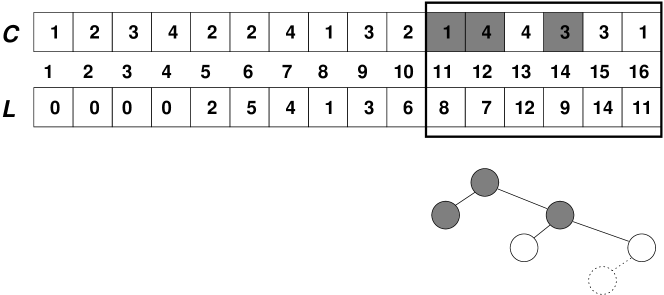
Figure 4: Color listing on $C[11,16]$ in our running example.

The algorithm is not only optimal time but also real time: As it reports the color before making the recursive calls, the top part of the Cartesian tree can be thought of as generated in preorder. Thus it takes $O(1)$ time to list each successive result.

Solution 4.13 (Color Listing)

[Muthukrishnan (2002)] The problem can be solved in linear space and real time.

In addition to this machinery, Mut02 uses a suffix tree on $\mathcal{T}$ to compute the interval $[sp,ep]$. This immediately gives an optimal solution to the document listing problem.

Solution 4.14 (Document Listing)

[Muthukrishnan (2002)] The problem can be solved in $O(m+\mathsf{docc})$ time and $O(n\lg n)$ bits of space.

Mut02 considered other more complex variants of the problem, such as listing the documents that contain $t$ or more occurrences of the pattern, or that contain two occurrences of the pattern within distance $t$. Those also lead to interesting, albeit more complex, algorithmic problems.

In practical terms, Mut02’s solution may use too much space, even if linear. It has been shown, however, that his very same idea can be implemented within much less space: just $O(n)$ bits on top of a CSA (Definition 3.6). We cover those developments in the next section.

5 Document Listing in Compressed Space

Sad07 addressed the problem of reducing the space of Mut02’s solution. He replaced the suffix tree by a CSA, and proposed the first RMQ solution that did not need to access $L$ (this one used $4n+o(n)$ bits; the one we have referenced in Solution 6 uses the optimal $2n+o(n)$). Thus array $L$ was not necessary for computing RMQs on it. Mut02’s algorithm, however, needs also to ask if $L[p]<sp$ in order to determine whether this is the first occurrence of color $C[p]$. Sad07 uses instead a bitmap $V[1,D]$ (set initially to all 0s), so that if $V[C[p]]=0$ then the document has not yet been reported, so we report it and set $V[C[p]]\leftarrow 1$.

Just as before, Sad07 ends the recursion at an interval $[i,j]$ when its minimum position $p$ satisfies $V[C[p]]=1$. There is a delicate point about the correctness of this algorithm, which is not stressed in that article. Replacing the check $L[p]<sp$ by $V[C[p]]=0$ only works if we first process recursively the left interval, $[i,p-1]$, and then the right interval, $[p+1,j]$. In this case one can see that the leftmost occurrence of each color is found and the algorithm visits the same cells of Mut02’s (we prove this formally in Appendix B, and also give an example where an error occurs otherwise).

Sad07’s technique yields the following solution, which uses $O(n)$ bits on top of the original array, as opposed to Mut02’s $O(n\lg n)$ bits used for $L$.

Solution 5.15 (Color Listing)

[Sadakane (2007)] The problem can be solved using $O(n)$ bits of space on top of array $C$, and in real time.

The reader may have noticed that we should reinitialize $V$ to all zeros before proceeding to the next query. A simple solution is to remember the documents output by the algorithm, so as to reset those entries of $V$ after finishing. This requires $\mathsf{docc}\lg D\leq D\lg D$ bits, which may be acceptable. Otherwise, array $V$ could be restored by rerunning the algorithm and using the bits with the reverse meaning. In practice, however, this doubles the running time. A more practical alternative is to use a classical solution to initialize arrays in constant time [Mehlhorn (1984)]. Although this solution requires $O(D\lg D)$ extra bits, we show in Appendix C how to reduce the space to $O(D)=O(n)$ bits, and even $D+o(D)$ bits.

By combining Solution 5.15 with any CSA, we also obtain a slightly improved version of Solution 4.14.

Solution 5.16 (Document Listing)

[Sadakane (2007)] The problem can be solved in time $O(t_{\mathsf{search}}(m)+\mathsf{docc})$ and $|\mathsf{CSA}|+n\lg D+O(n)$ bits of space, where $\mathsf{CSA}$ is a CSA indexing $\mathcal{D}$.

Note that we have removed array $L$, but $C$ is still used to report the actual colors. For the specific case of document listing, Sad07 also replaced array $C$ by noticing that it can be easily computed from the CSA and a bitmap $B[1,n]$ that marks with 1s the positions of the “$” symbols in $\mathcal{T}$. Then, using the $\mathsf{rank}$ operation (Problem 4) we compute $C[i]=1+\mathsf{rank}_{1}(B,A[i]-1)$. While $\mathsf{rank}$ can be computed in constant time (Solution 1), the computation of $A[i]$ using the CSA (Definition 3.6) requires time $t_{\mathsf{SA}}$. Overall, the following result is obtained.

Solution 5.17 (Document Listing)

[Sadakane (2007)] The problem can be solved in time $O(t_{\mathsf{search}}(m)+\mathsf{docc}\,t_{\mathsf{SA}})$ and $|\mathsf{CSA}|+O(n)$ bits of space, where $\mathsf{CSA}$ is a CSA indexing $\mathcal{D}$.

Example 5.18

Fig. 5 illustrates the components of Sad07’s solution.

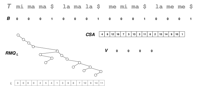
Figure 5: The structures for document listing in compressed space, on our running example. The grayed structures are not stored. We draw the Cartesian tree of $L$ to represent $\textsc{rmq}_{L}$.

HSV09 managed to reduce the $O(n)$-bit term in the space complexity to just $o(n)$. They group $b$ consecutive entries in $L$. Then they create a sampled array $L^{\prime}[1,n/b]$ where each entry contains the minimum value in the corresponding block of $L$. The RMQ data structure is built over $L^{\prime}$, and they run the algorithm over the blocks that are fully contained in $L[sp,ep]$. Each time a position in $L^{\prime}$ is reported, they consider all the $b$ entries in the corresponding block of $L$, reporting all the documents that have not yet been reported. Only if all of them have already been reported can the recursion stop. They also process by brute force the tails of the interval $L[sp,ep]$ that overlap blocks. Therefore they have a multiplicative time overhead of $O(b)$ per document reported, in exchange for reducing the $O(n)$-bit space to $O(n/b)$.

This idea only works if we first process the left subinterval, then mark the documents in the block where the minimum was found, and then process the right subinterval, for the same delicate reason we have described on Sad07’s method. Otherwise, marking as visited other documents than the one holding the minimum $L$ value (namely all others in the block) can make the recursion stop earlier than it should. We prove the correctness of this technique in Appendix D, where we also show that the result can be incorrect if applied in a different order.

The other $O(n)$ bits of space come from the bitmap $B$ that marks the positions of terminators in $\mathcal{T}$. Since $B$ has only $D$ bits set, it is easily represented in compressed form using Solution 2.

Solution 5.19 (Document Listing)

[Hon et al. (2009)] The problem can be solved in time $O(t_{\mathsf{search}}(m)+\mathsf{docc}\,t_{\mathsf{SA}}\lg^{\epsilon}n)$ and $|\mathsf{CSA}|+D\lg(n/D)+O(D)+o(n)$ bits of space, where $\mathsf{CSA}$ is a CSA indexing $\mathcal{D}$, for any constant $\epsilon>0$.

6 Computing Term Frequencies

As explained in the Introduction, the term frequency $\mathsf{tf}(P,d)$ is a key component in many relevance formulas, and thus the problem of computing it for the documents that are output by a document listing algorithm is relevant. In terms of the document array, this leads to the following problem on colors, which as explained has its own important applications in various data mining problems.

Problem 6.20 (Color Listing with Frequencies)

Preprocess an array $C[1,n]$ of colors in $[1..D]$ so that, given a range $[sp,ep]$, we can output the distinct colors in $C[sp,ep]$, each with its frequency in this range.

Given a color $d$, computing its frequency in $C[sp,ep]$ is easily done via $\mathsf{rank}$ operations (Problem 4): $\mathsf{rank}_{d}(C,ep)-\mathsf{rank}_{d}(C,sp-1)$. Therefore, any solution to color listing (e.g., Solution 5.15) plus any solution to computing $\mathsf{rank}$ on sequences (e.g., Solution 4) yields a solution to color listing with frequencies. Indeed, Solution 4 is close to optimal [Belazzougui and Navarro (2012)]. Thus, one can solve color listing with frequencies using $o(n\lg D)$ additional bits and $O(\lg\lg D)$ per color output.

Somewhat surprisingly, the problem can be solved faster by noticing that we do not need the full power of $\mathsf{rank}$ queries on $C$. BNV13 replace the $\mathsf{rank}$-enabled sequence representation of $C$ by a weaker representation using less space and time, but sufficient for this purpose. They use one mmphf $B_{d}$ (recall Solution 3) for each color $d$, marking the positions $B_{d}[i]=1$ where $C[i]=d$. Then, if one knew that $i$ and $i^{\prime}$ are the first and last occurrences of color $d$ in $C[sp,ep]$, one could compute the color frequency as $\mathsf{rank}_{1}(B_{d},i^{\prime})-\mathsf{rank}_{1}(B_{d},i)+1$.

Note that Mut02’s algorithm naturally finds the leftmost occurrence $i$. With a different aim, Sad07 had shown how to compute the rightmost occurrence $i^{\prime}$. He creates another RMQ (now meaning range maximum query) structure over a variant of $L$ where each element points to its successor rather than its predecessor. Run over this new RMQ, Mut02’s algorithm will find $i^{\prime}$ instead of $i$, for each document $d$ in $C[sp,ep]$.

Sad07 then uses sorting to match the $i$ and $i^{\prime}$ position of each document $d$, whereas BNV13 avoids the sorting but uses $O(D\lg n)$ further bits. In Appendix E we show how both can be avoided with a dictionary that takes just $O(\lg D)$ bits per listed color plus $o(D)$ total space. In this dictionary we insert the leftmost occurrences (with document identifiers as keys) and later search for the rightmost occurrences. Then, by using the faster variant of Solution 3, BNV13 obtain the following result.

Solution 6.21 (Color Listing with Frequencies)

[Belazzougui et al. (2013)] The problem can be solved in optimal time and $O(n\lg\lg D)$ bits on top of array $C$.

Note that, compared to Solution 5.15, that listed the colors without frequencies, the real time has become “just” optimal, and the extra space of $O(n)$ bits has increased, yet it is still $o(n\lg D)$ as long as $D=o(n)$. Note also that this solution cannot compute the frequency of an arbitrary color, but only of those output by the color listing algorithm.

The corresponding problem on documents is defined as follows.

Problem 6.22 (Document Listing with Frequencies)

Preprocess a document collection $\mathcal{D}$ so that, given a pattern string $P$, one can compute $\{(d,\mathsf{df}(P,d)),\mathsf{df}(P,d){>}0\}$.

VM07 were the first to propose reducing this problem to color listing with frequencies on the document array $C$. Their most interesting idea is that the whole document listing problem can be reduced to $\mathsf{rank}$ and $\mathsf{select}$ operations on $C$: Array $L$ can be simulated as $L[i]=\mathsf{select}_{C[i]}(C,\mathsf{rank}_{C[i]}(C,i)-1)$. Thus, they simulate the original document listing algorithm of Mut02 over this representation of $L$, using the $O(n)$-bit RMQ of Solution 6, and using a CSA (Definition 3.6) to obtain the range $C[sp,ep]$. Although they used wavelet trees (Definition 4) to represent $C$, using instead Solution 4 yields the following result.

Solution 6.23 (Document Listing with Frequencies)

[Välimäki and Mäkinen (2007)] The problem can be solved in time $O(t_{\mathsf{search}}(m)+\mathsf{docc}\,\lg\lg D)$ and $|\mathsf{CSA}|+n\lg D+o(n\lg D)$ bits of space, where $\mathsf{CSA}$ is a CSA indexing $\mathcal{D}$.

Combining this idea with Solution 6.21, so that we need only constant-time access to $C$, we immediately obtain a time-optimal solution.

Solution 6.24 (Document Listing with Frequencies)

[Belazzougui et al. (2013)] The problem can be solved in time $O(t_{\mathsf{search}}(m)+\mathsf{docc})$ and $|\mathsf{CSA}|+n\lg D+o(n\lg D)$ bits of space, where $\mathsf{CSA}$ is a CSA indexing $\mathcal{D}$.

Still, the space is much higher than the near-optimal one of Solutions 5.17 and 5.19. The document array is usually much larger than the text or its CSA. Sad07 proposed instead a solution that, once the leftmost and rightmost positions $i$ and $i^{\prime}$ of document $d$ are known, computes $\mathsf{tf}(P,d)$ using the local CSA of document $d$. This doubles the total CSA space, but avoids storing the document array. We describe this solution in Appendix F.

Solution 6.25 (Document Listing with Frequencies)

[Sadakane (2007)] The problem can be solved in time $O(t_{\mathsf{search}}(m)+\mathsf{docc}\,t_{\mathsf{SA}})$ and $2|\mathsf{CSA}|+O(n)$ bits of space, where $\mathsf{CSA}$ is a CSA indexing $\mathcal{D}$.

If we use the mmphf-based solution of BNV13 to compute the frequencies, instead of doubling the CSA space, the following results are obtained by using variants of Solution 3.

Solution 6.26 (Document Listing with Frequencies)

[Belazzougui et al. (2013)] The problem can be solved in time $O(t_{\mathsf{search}}(m)+\mathsf{docc}\,t_{\mathsf{SA}})$ and $|\mathsf{CSA}|+O(n\lg\lg D)$ bits of space, where $\mathsf{CSA}$ is a CSA indexing $\mathcal{D}$. By adding $O(\mathsf{docc}\lg\lg D)$ time, the space can be reduced to $|\mathsf{CSA}|+O(n\lg\lg\lg D)$ bits.

All the solutions described build over the original algorithm of Mut02. There is another line of solutions that, although not much competitive in terms of complexities, yields good practical results and builds on different ideas. We describe this thread in Appendix G; the main result obtained follows.

Solution 6.27 (Document Listing with Frequencies)

[Gagie et al. (2012)] The problem can be solved in time $O(t_{\mathsf{search}}(m)+\mathsf{docc}\,\lg(D/\mathsf{docc}))$ and $|\mathsf{CSA}|+n\lg D+o(n\lg D)$ bits of space, where $\mathsf{CSA}$ is a CSA indexing $\mathcal{D}$.

We note that, while document listing could be carried out within just $o(n)$ extra bits on top of the CSA, reporting frequencies requires significantly more space. This is similar to what we observed for color listing. In Appendix I (Solution 10.57) we will show how to use the solutions for top-$k$ retrieval to perform document listing with frequencies using only $o(n)$ bits on top of the CSA.

7 Computing Document Frequencies

Document frequency $\mathsf{df}(P)$, the number of distinct documents where a pattern occurs, is used in many variants of the tf-idf weighting formula, as mentioned in the Introduction. In other contexts, such as pattern mining, it is a measure of how interesting a pattern is.

Problem 7.28 (Document Frequency)

Preprocess a document collection $\mathcal{D}$ so that, given a pattern $P$, one can compute $\mathsf{df}(P)$, the number of documents where $P$ appears.

Sad07 showed that this problem has a good solution. One can store $2n+o(n)$ bits associated to the GST of $\mathcal{D}$ so that $\mathsf{df}(P)$ can be computed in constant time once the locus node of $P$ is known. We describe his solution in Appendix H.

Solution 7.29 (Document Frequency)

[Sadakane (2007)] The problem can be solved in $O(t_{\mathsf{search}}(m))$ time using $|\mathsf{CSA}|+O(n)$ bits of space.

On the other hand, in terms of the document array, computing document frequency leads to the following problem, which is harder but of independent interest.

Problem 7.30 (Color Counting)

Preprocess an array $C[1,n]$ of colors in $[1..D]$ so that, given a range $[sp,ep]$, we can compute the number of distinct colors in $C[sp,ep]$.

This problem is also called categorical range counting and it has been recently shown to require at least $\Omega(\lg n/\lg\lg n)$ time if using space $O(n\,\textrm{polylog}(n))$ [Larsen and van Walderveen (2013)]. Indeed, it is not difficult to match this lower bound: By Lemma 4.11, it suffices to count the number of values smaller than $sp$ in $L[sp,ep]$ [Gupta et al. (1995)]. This is a well-known geometric problem, which in simplified form follows.

Problem 7.31 (Two-Dimensional Range Counting)

Preprocess an $n\times n$ grid of $n$ points so that, given a range $[r_{1},r_{2}]\times[c_{1},c_{2}]$, we can count the number of points in the range.

Our problem on $L$ becomes a two-dimensional range counting problem if we consider the points $(L[i],i)$. Then our two-dimensional range is $[0,sp-1]\times[sp,ep]$.

Example 7.32

Fig. 6 shows the grid corresponding to array $L$ in our running example, where we have highlighted the query corresponding to $C[11,16]$. As expected, two-dimensional range counting indicates that there are $3$ points in $[0,10]\times[11,16]$, and thus $3$ distinct colors in $C[11,16]$.

Figure 6: The grid representation of array $L$ in our running example.

Two-dimensional range counting has been solved in $O(\lg n/\lg\lg n)$ time and $n\lg n+o(n\lg n)$ bits of space by BHMM09. Unsurprisingly, this time is also optimal within $O(n\,\textrm{polylog}(n))$ space [Pătraşcu (2007)].

Solution 7.33 (Color Counting)

[Gupta et al. (1995), Bose et al. (2009)] The problem can be solved in $O(\lg n/\lg\lg n)$ time and $n\lg n+o(n\lg n)$ bits of space.

We note that the space in this solution does not account for the storage of the color array $C[1,n]$ itself, but it is additional space (the solution does not need to access $C$, on the other hand). GKNP13 used this same reduction, but resorting to binary wavelet trees instead of the faster data structure of BHMM09 Instead, they reduced the $n\lg n$ bits of this wavelet tree, and also made the time dependent on the query range (we ignore compressibility aspects of their results).

Solution 7.34 (Color Counting)

[Gagie et al. (2013)] The problem can be solved in $O(\lg(ep-sp+1))$ time and $n\lg D+o(n\lg D)+O(n)$ bits of space.

Again, this result does not consider (nor needs) the storage of the array $C$ itself.

8 Most Important Document Retrieval

We move on now from the problem of listing all the documents where a pattern occurs to that of listing only the $k$ most important ones. In the simplest scenario, the documents have assigned a fixed importance, as defined in Problem 3. By means of the document array, this can be recast into the following problem on colors.

Problem 8.35 (Top-$k$ Heaviest Colors)

Preprocess an array $C[1,n]$ of colors in $[1..D]$ with weights in $W[1,D]$ so that, given a range $[sp,ep]$ and a threshold $k$, we can output $k$ distinct colors with highest weight in $C[sp,ep]$.

A first observation is that, if we reorder the colors so that their weights $W$ become decreasing, $W[d]\geq W[d+1]$, then the problem becomes that of reporting the $k$ colors with lowest identifiers in $C[sp,ep]$. This is indeed achieved by GPT09 using consecutive range quantile queries on wavelet trees, as explained in Appendix G (Solution G.65), and it is easy to adapt the subsequent improvement [Gagie et al. (2012)] to stop after the first $k$ documents are reported. It is not hard to infer the following result, where the wavelet tree can also reproduce any cell of $C$ (and thus replace $C$, if we accept its access time).

Solution 8.36 (Top-$k$ Heaviest Colors)

[Gagie et al. (2012)] The problem can be solved in $O(k\,\lg(D/k))$ time and $n\lg D+o(n\lg D)$ bits of space. Within this space we can access any cell of $C$ in time $O(\lg D)$.

Note that this assumes that we can freely reorder the colors. If this is not the case we need other $D\lg D$ bits to store the permutation. On the other hand, by spending linear space ($O(n\lg n)$ bits), we can use the improved range quantile algorithms of BGJS11. In this case, however, an optimal-time solution by KN11 is preferable.

Solution 8.37 (Top-$k$ Heaviest Colors)

[Karpinski and Nekrich (2011)] The problem can be solved in real time and $O(n\lg D)$ bits of space.

Therefore, we obtain the following results for document retrieval problems.

Solution 8.38 (Top-$k$ Most Important Documents)

[Karpinski and Nekrich (2011)] The problem can be solved in time $O(t_{\mathsf{search}}(m)+k)$ and $|\mathsf{CSA}|+O(n\lg D)$ bits of space, where $\mathsf{CSA}$ is a CSA indexing $\mathcal{D}$.

Solution 8.39 (Top-$k$ Most Important Documents)

[Gagie et al. (2012)] The problem can be solved in time $O(t_{\mathsf{search}}(m)+k\,\lg(D/k))$ and $|\mathsf{CSA}|+n\lg D+o(n\lg D)$ bits of space, where $\mathsf{CSA}$ is a CSA indexing $\mathcal{D}$.

We defer the results using compressed space to Section 10 (Solution 10.52).

9 Top-$k$ Document Retrieval

We now consider the general case, where the weights of the documents may depend on $P$ as well. HSV09 introduced a fundamental framework to solve this general top-$k$ document retrieval problem. All the subsequent work can be seen as improvements that build on their basic ideas (see HPSW10 for prior work).

Their basic construction enhances the GST of the collection $\mathcal{D}$ so that the local suffix tree of each document $T_{d}$ is embedded into the global GST. More precisely, let $u$ be a node of the suffix tree of document $T_{d}$, and let $w$ be its parent in that suffix tree. Further, let $\mathsf{occ}(u)=\mathsf{tf}(u,d)$ be the number of leaves below $u$ in the suffix tree of $T_{d}$. There must exist nodes $u^{\prime}$ and $w^{\prime}$ in the GST of $\mathcal{D}$ with the same string labels, $str(u^{\prime})=str(u)$ and $str(w^{\prime})=str(w)$. Then we record a pointer labeled $d$ from $u^{\prime}$ to $w^{\prime}$, with weight $\mathsf{occ}(u)$. Thus the set of parent pointers for each document $d$ forms a subgraph of the GST that is isomorphic to the suffix tree of $T_{d}$. From the fact that the pointers labeled $d$ correspond to an embedding of the suffix tree of $T_{d}$ into the GST, the following crucial lemma follows easily.

Lemma 9.40

[Hon et al. (2009)] Let $v$ be a nonroot node in the GST of $\mathcal{D}$. For each document $d$ where $str(v)$ occurs $\mathsf{tf}(v,d)>0$ times, there exists exactly one pointer from the subtree of $v$ (including $v$) to a proper ancestor of $v$, labeled $d$ and with weight $\mathsf{tf}(v,d)$.

To see this, note that if $str(v)$ occurs in $T_{d}$, there must be a node $u$ of the suffix tree of $T_{d}$ mapped to $u^{\prime}$ in GST, which is below $v$ (or is $v$ itself). If we follow the successive upward pointers from $u^{\prime}$, we go over $v$ at some point, so there must be at least one such pointer from a subtree of $v$ to a proper ancestor of $v$. On the other hand, there cannot be two such pointers leaving from $u^{\prime\prime}$ and $u^{\prime\prime\prime}$, because the LCA of both nodes must also be in the suffix tree of $T_{d}$, and hence $u^{\prime\prime}$ and $u^{\prime\prime\prime}$ must point to this LCA or below it. But since $u^{\prime\prime}$ and $u^{\prime\prime\prime}$ descend from $v$, their LCA also descends from $v$, so their pointers point at or below $v$. Notice, moreover, that the source $u^{\prime}$ of this unique pointer has a weight $\mathsf{tf}(u,d)$, which must be $\mathsf{tf}(v,d)$, since all the occurrences of $v$ in document $d$ are in nodes below $u^{\prime}$ in the GST.

Example 9.41

Fig. 7 illustrates how the suffix tree of document $T_{1}$ is embedded in the GST, in our running example. The upward pointers describe the topology of the local suffix tree. Note that for all the patterns that appear in $T_{1}$, such as ”ma”, ”mi ma”, and ”ma ma”, but not ”la” nor ”me”, there is exactly one upward pointer leaving from the subtree of the locus and arriving at an ancestor of the locus.

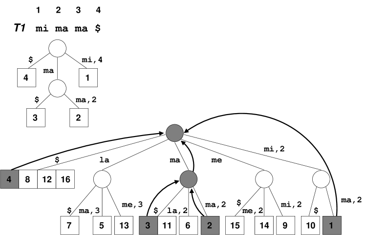
Figure 7: The embedding of the suffix tree of $T_{1}$ in the global GST. The nodes are shown grayed and the upward pointers as thick arrows.

HSV09 store the pointers at their target nodes, $w^{\prime}$. Thus, given a pattern $P$, we find its locus $v$ in the GST, and then the ancestors $v_{1},v_{2},\ldots$ of $v$ record exactly one pointer labeled $d$ per document where $P$ appears, together with the weight $\mathsf{tf}(P,d)$. However, we only want those pointers that originate in nodes $u^{\prime}$ within the subtree of $v$. For this sake, the pointers arriving at each node $w^{\prime}$ are stored in preorder of the originating nodes $u^{\prime}$, and thus those starting from descendants $u^{\prime}$ of $v$ form a contiguous range in the target nodes $w^{\prime}$. Furthermore, we build RMQ data structures (this time choosing maxima, not minima) on the $\mathsf{tf}(P,d)$ values associated to the pointers. Fig. 8 (left) illustrates the scheme.

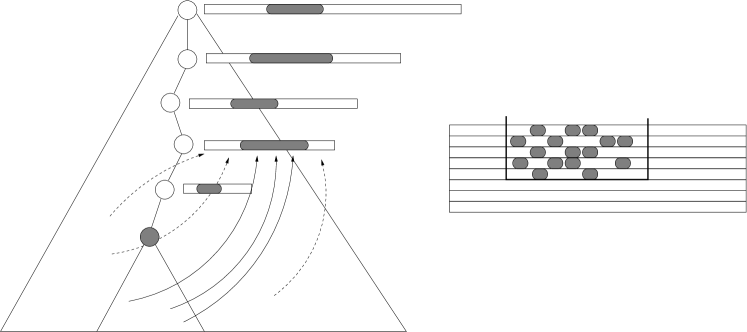
Figure 8: The linear-space schemes for top-$k$ documents. On the left, the GST with the locus node shadowed. From the arrays of its ancestors (targets of pointers) we choose the areas (shadowed) of those leaving from the subtree of the locus. We draw the pointers that go to the grandparent of the locus. Solid arrows leave from the subtree of the locus and dashed ones from other descendants of the grandparent node. On the right, the mapping of those arrays into a grid, where the row is the depth of the target and the column is the preorder of the source.

The node $v$ has at most $m$ ancestors. In principle we have to binary search those $m$ arrays to isolate the ranges of the pointers leaving from the subtree of $v$. A technical improvement reduces the time to find those ranges from $O(m\lg D)$ to $O(m)$ time, let $v_{i}[sp_{i},ep_{i}]$ be those ranges. Then, with an RMQ on each such interval we obtain the positions $p_{i}$ where the maximum weight in each such array occurs. Those $m$ weights are inserted into a max-priority queue bounded to size $k$ (i.e., the $(k+1)$th and lower weights are always discarded). Now we extract the maximum from the queue, which is the top-1 answer. We go back to its interval $v_{i}[sp_{i},ep_{i}]$ and cut it into two, $v_{i}[sp_{i},p_{i}-1]$ and $v_{i}[p_{i}+1,ep_{i}]$, compute their RMQ positions, and reinsert them in the queue. After repeating this process $k$ times, we have obtained the top-$k$ documents.

Solution 9.42 (Top-$k$ Documents)

[Hon et al. (2009)] The problem can be solved in $O(m+k\lg k)$ time and $O(n\lg n)$ bits of space.

Example 9.43

Fig. 9 shows the arrays of target nodes, in the format $(d,\mathsf{tf}(u^{\prime},d))$, sorted by preorder of the source nodes but omitting the preorder information for clarity. We shadow the locus node $v$ of $P=\textsf{"ma"}$. In this small example the locus has only one proper ancestor, the root $v_{1}$. The range $v_{1}[sp_{1},ep_{1}]=v_{1}[7,9]$ in that array corresponds to the pointers leaving from the subtree of $v$. An RMQ structure over this array lets us find in constant time the top-1 answer, $v_{1}[7]=(d=1,\mathsf{tf}(P,d)=2)$. To get the top-2 answer we split the interval into $v_{1}[7,6]$ (empty) and $v_{1}[8,9]$, and pick the largest of the two.

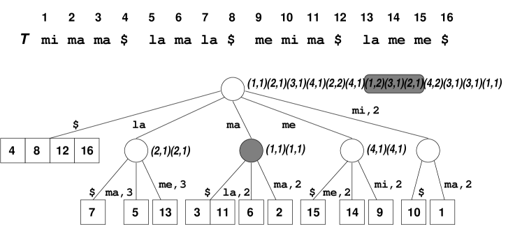
Figure 9: The locus of $P=\textsf{"ma"}$ and the area of the list that corresponds to it.

Note that the weights $\mathsf{tf}(P,d)$ can be replaced by any other measure that is a function of the locus of $P$ in the suffix tree of $T_{d}$. This includes some as sophisticated as $\mathsf{dmin}(P,d)$, the minimum distance between any two occurrences of $P$ in $d$.

NN12 improved the space and time of this solution by using a different way of storing the pointers. They consider a grid of size $O(n)\times O(n)$ so that a pointer from node $u^{\prime}$ to node $w^{\prime}$ is stored as a point $(\mathit{depth}(w^{\prime}),\mathit{preorder}(u^{\prime}))$ in this grid, associated to the document $d$ and with weight $\mathsf{tf}(u^{\prime},d)$. Then, once the locus $v$ of $P$ is found in the suffix tree, the problem is reduced to that of finding the $k$ heaviest points in the range $[0,\mathit{depth}(v)-1]\times[\mathit{preorder}(v),\mathit{preorder}(v)+\mathit{subtreesize}(v)-1]$ on the grid (note that there may be several points in a single place of this grid, which can be dealt with by creating unique columns for them). This is, again, a geometric problem. We illustrate it in Fig. 8 (right).

The key to achieving optimal time is to note that the height of the query range is at most $m$, and we have already spent $O(m)$ time to find the pattern. NN12 show that, if we can spend time proportional to the row-size of the query range, then it is possible to report each top-$k$ point in constant time. In addition, they manage to slightly reduce the space.

Solution 9.44 (Top-$k$ Documents)

[Navarro and Nekrich (2012)] The problem can be solved in $O(m+k)$ time and $O(n(\lg D+\lg\sigma))$ bits of space.

Other weights than $\mathsf{tf}(P,d)$ can also be used in this (and also HSV09’s) solution, yet the space here becomes $O(n(\lg D+\lg\sigma+\lg\lg n))$ bits.

Example 9.45

Fig. 10 illustrates NN12’s representation of the pointers on a grid. In our example the grid is just of height two, and there is no more than one pointer per cell. The query area is shaded.

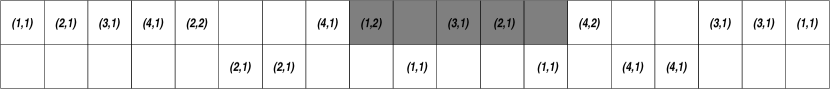
Figure 10: The grid representation of the pointers and the query.

We note that Solutions 9.42 and 9.44 are online, that is, we do not need to specify $k$ in advance, but can run the algorithms and stop them at any time, after reporting $k$ documents. Interestingly, the optimal online solution immediately yields optimal solutions to various outstanding challenges left open by Mut02. First, if we want to list all the documents where a pattern appears more than $t$ times, we simply run the online algorithm until it outputs the first document $d$ with $\mathsf{tf}(P,d)<t$. Second, if we want to list all the documents where two occurrences of the pattern appear within distance at most $t$, we do the same with the $\mathsf{dmin}$ weighting function. Mut02 had obtained sophisticated solutions for those problems, which were optimal-time and linear-space only for $t$ fixed at index construction time. Now we can solve those problems as particular cases, in linear space and optimal time, defining $t$ at query time, and even in online form.

Mut02’s solutions, on the other hand, work for general color range problems, not only for document retrieval. This opens the question of whether we can also solve the corresponding top-$k$ problem on colors.

Problem 9.46 (Top-$k$ Colors)

Preprocess an array $C[1,n]$ of colors in $[1..D]$ so that, given a range $[sp,ep]$ and a threshold $k$, we can output $k$ colors with highest frequency in $C[sp,ep]$.

For $k=1$ this problem is called the range mode problem. The best exact solution is by CDLMW12, who achieve linear space but a high time, $O(\sqrt{n/\lg n})$. The problem admits, however, good approximations. An $(1+\epsilon)$-approximation to the range mode problem is to find an element whose frequency is at least $1+\epsilon$ times less than that of the range mode. GJLT10 show that one can find such an approximation in $O(\lg(1/\epsilon))$ time and $O((n/\epsilon)\lg n)$ bits of space.

GKNP13 extends the solution to find approximate top-$k$ colors, where one guarantees that no ignored color occurs more than $1+\epsilon$ times than a reported color. The technique composes the approximate solution for top-1 color with a wavelet tree on $C$ (Definition 4), so that one such structure is stored for each sequence $C_{v}$ associated to wavelet tree node $v$. For the top-1 answer, say $d_{1}$, it is sufficient to query the root. For the top-2 answer, $d_{2}$, we must exclude $d_{1}$ from the solution. This is done by considering all the siblings of the nodes in the path from the root to the leaf $d_{1}$ of the wavelet tree. The maximum over all those top-1 queries gives the top-2. For the top-3, we must repeat the process to exclude also $d_{2}$ from the set, and so on. We maintain a priority queue with all the wavelet tree nodes that are candidates for the next answer. After returning $k$ answers, the queue has $k\lg D$ candidates (as the root-to-leaf paths are of length $\lg D$). By using an appropriate priority queue implementation, Solution 9.47 is obtained.

Solution 9.47 (Top-$k$ Colors)

[Gagie et al. (2013)] An $(1+\epsilon)$-approximation for the problem takes $O(k\lg D\lg(1/\epsilon))$ time and $O((n/\epsilon)\lg D\lg n)$ bits of space.

Example 9.48

Fig. 11 illustrates the process. On the left, we query $C[4,13]$, finding on the root that $4$ is the most frequent color. To find the top-2 result, we remove $4$ from the alphabet by partitioning the root node (which handles symbols $[1..4]$) into two wavelet tree nodes: that handling $[1..2]$ and that handling $[3]$ (on the right). Now we perform the query on both arrays, finding that $2$ is the most frequent color from both nodes. If we wanted the top-3, it would be decided between wavelet tree leaves handling $[1]$ and $[3]$.

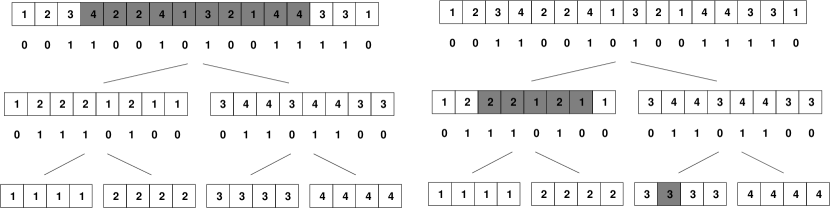
Figure 11: The process of solving top-$k$ colors.

This result is not fully satisfactory for two reasons. First, the space is super-linear. Second, it is approximate. The second limitation, however, seems to be intrinsic. CDLMW12 show that it is unlikely, even for $k=1$, to obtain times below $\Theta(n^{\omega/2-1})$ using space below $\Theta(n^{\omega/2})$, where $\omega$ is the matrix multiplication exponent (best known value is $\omega=2.376$). This is a case where document retrieval queries, which translate into specific colored range queries (where the possible queries come from a tree) are much easier than general colored range queries.

On the other hand, there has been much research, and very good results, on solving the top-$k$ documents problem in compressed space (for the $\mathsf{tf}$ measure). We describe the most important results next.

10 Top-$k$ Document Retrieval in Compressed Space

In their seminal paper, HSV09 also presented the first compressed solution to the top-$k$ document retrieval problem under measure $\mathsf{tf}$. The idea is to sample some suffix tree nodes and store the top-$k$ answer for those sampled nodes. The sampling mechanism guarantees that this answer must be “corrected” with just a small number of suffix tree leaves in order to solve any query.

Assume for a moment that $k$ is fixed and let $b=k\lg^{2+\epsilon}n$. We choose the GST leaves whose suffix array position is a multiple of $b$, and mark the LCA of each pair of consecutive chosen leaves. This guarantees that the LCA of any two chosen leaves is also marked. At each of the $n/b$ marked internal nodes $v$, we store the result $\mathsf{top}(\mathcal{D},str(v),k)$. This requires $O(k\lg n)$ bits per sampled node, which adds up to $O(n/\lg^{1+\epsilon}n)$ bits. The subgraph of the GST formed by the marked nodes (preserving ancestorship) is called $\tau_{k}$.

Instead of storing the GST, we store the trees $\tau_{k}$, for all $k$ values that are powers of 2. All the $\tau_{k}$ trees add up to $O(n/\lg^{\epsilon}n)=o(n)$ bits. Given a top-$k$ query, we solve it in tree $\tau_{k^{\prime}}$, where $k^{\prime}=2^{\lceil\lg k\rceil}=O(k)$ is the power of 2 next to $k$.

Just as the pattern $P$ has a locus node $v$ in the GST, it has a locus $v^{\prime}$ in $\tau_{k^{\prime}}$, using the same Definition 3.3. It is not hard to see that, since the nodes of $\tau_{k^{\prime}}$ are a subset of those of the GST, $v^{\prime}$ must descend from $v$ (or be the same). A way to find $v^{\prime}$ is to use a CSA and obtain the range $[sp,ep]$ of $P$, then restrict it to the closest multiples of $b^{\prime}=k^{\prime}\lg^{2+\epsilon}n$, $[sp^{\prime\prime},ep^{\prime\prime}]\subseteq[sp,ep]$, then take the $(sp^{\prime\prime}/b)$th and $(ep^{\prime\prime}/b)$th leaves of $\tau_{k^{\prime}}$, and finally take $v^{\prime}$ as the LCA of those two leaves. The following property is crucial.

Lemma 10.49

[Hon et al. (2009)] The node $v^{\prime}\in\tau_{k^{\prime}}$ covers a range $[sp^{\prime},ep^{\prime}]$ such that $[sp^{\prime\prime},ep^{\prime\prime}]\subseteq[sp^{\prime},ep^{\prime}]\subseteq[sp,ep]$.

It holds that $[sp^{\prime\prime},ep^{\prime\prime}]\subseteq[sp^{\prime},ep^{\prime}]$ because $v^{\prime}$ is the LCA of leaves $sp^{\prime\prime}$ and $ep^{\prime\prime}$ in the GST, and it holds that $[sp^{\prime},ep^{\prime}]\subseteq[sp,ep]$ because $v$ is the LCA of $[sp,ep]$ and it is an ancestor of $v^{\prime}$. Moreover, note that $sp^{\prime}-sp\leq b$ and $ep-ep^{\prime}\leq b$.

Node $v^{\prime}$ has precomputed the top-$k$ answer for $[sp^{\prime},ep^{\prime}]$ (moreover, the top-$k^{\prime}$ answer). We only need to correct this list with the documents that are mentioned in $A[sp,sp^{\prime}-1]$ and $A[ep^{\prime}+1,ep]$, and those ranges are shorter than $b$. It is also possible that $[sp^{\prime\prime},ep^{\prime\prime}]=\emptyset$, but in this case it holds that $[sp,ep]$ is shorter than $2b$ and thus the answer can be computed from scratch by examining those $O(b)$ cells. Fig. 12 illustrates the scheme. The locus $v$ is in gray and the marked node $v^{\prime}$ in black. The areas that must be traversed sequentially are in bold.

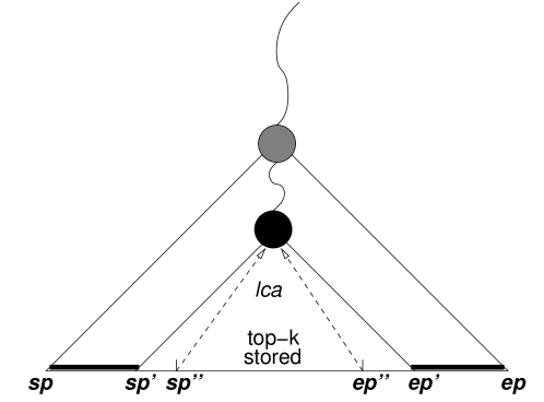
Figure 12: The compressed top-$k$ retrieval scheme.

In the general case, we have up to $k$ precomputed candidates and must correct the answer with $O(b)$ suffix array cells. We traverse those cells one by one and compute the corresponding document $d$ using $A$ as in Solution 5.17. Now, each such document $d$ may occur many more times in $C[sp^{\prime},ep^{\prime}]$, yet be excluded from the top-$k$ precomputed list. Therefore, we need a mechanism to compute its frequency $\mathsf{tf}(P,d)$ in $C[sp,ep]$. Note that we cannot use the technique of Solution 6.25, because we do not have access to the first and last occurrence of $d$ in $C[sp,ep]$.

We do have access, however, to either the first (if we are scanning $C[sp,sp^{\prime}-1]$) or the last (if we are scanning $C[ep^{\prime}+1,ep]$) position of $d$ in $C[sp,ep]$. Appendix F explains how HSV09 compute $\mathsf{tf}(P,d)$ in $O(t_{\mathsf{SA}}\,\lg n)$ time in this case. Once we know the frequency, we can consider including $d$ in the top-$k$ candidate list (note $d$ might already be in the list, in which case we have to update its original frequency, which only considers $C[sp^{\prime},ep^{\prime}]$). This yields a total cost of $O(b\,t_{\mathsf{SA}}\lg n)$ time to solve the query. By using a compressed bitmap representation (Solution 2) for the bitmap $B$ that marks the document beginnings, we obtain the following result.

Solution 10.50 (Top-$k$ Documents)

[Hon et al. (2009)] The problem can be solved in time $O(t_{\mathsf{search}}(m)+k\,t_{\mathsf{SA}}\lg^{3+\epsilon}n)$ and $2|\mathsf{CSA}|+D\lg(n/D)+O(D)+o(n)$ bits of space, where $\mathsf{CSA}$ is a CSA indexing $\mathcal{D}$, for any constant $\epsilon>0$.

Note that the space simplifies to $2|\mathsf{CSA}|+o(n)$ if $D=o(n)$. There have been several technical improvements over this idea [Gagie et al. (2013), Belazzougui et al. (2013)]. The best current results, however, have required deeper improvements.

One remarkable idea arised when extending the mmphfs of Solution 6.26 to top-$k$ retrieval. The idea of BNV13 is that, if a document $d$ occurs in the left ($[sp,sp^{\prime}-1]$) and the right ($[ep^{\prime}+1,ep]$) tails of the interval, then we know its first and last occurrence in $C[sp,ep]$, and thus the mmphfs can be used to compute $\mathsf{tf}(P,d)$ fast. The problem are the documents $d$ that appear only in one of the tails. BNV13 prove, however, that there can be only $k+\sqrt{2bk}$ elements of this kind that can make it to the top-$k$ list.

To see this, let $f_{min}$ be the $k$th frequency in the top-$k$ stored set. Then all the other documents have frequency $\leq f_{min}$. The first $k$ documents of the tail can immediately enter the list, if they now reach frequency $f_{min}+1$. However, the next documents to enter the top-$k$ list must now reach frequency $f_{min}+2$, and thus we need to scan at least $2k$ cells of the tail to complete the next batch of $k$ candidates. Similarly, the next $k$ candidates require scanning at least $3k$ cells to reach frequency $f_{min}+3$, and so on. To incorporate $sk$ elements we need to scan $\Omega(s^{2}k)$ cells. Since we scan at most $b$ cells, the bound $O(\sqrt{bk})$ follows.

With some care, the frequency of all those potential candidates can be stored as well (for example, their frequency must be in the narrow range $[f_{min}-b+1,f_{min}]$, and instead of storing the document identifiers $d$ we can mark one of their occurrences in $[sp,sp^{\prime}-1]$ or $ep^{\prime}+1,ep]$, either of length at most $b$. We can then obtain $d$ using the CSA, using only $O(\lg\lg n)$ bits to specify $d$ and its frequency.

Recently, Tsu13 improved this result further, by noticing that the idea of limiting the number of candidates can be extended to the case where the document appears in both tails. This is because the only interesting ranges are those that correspond to GST nodes, and the leaves covered by the successive unmarked ancestors of $v^{\prime}$ (until reaching the nearest marked ancestor) form $O(b)$ increasing sets of leaves, so the reasoning of BNV13 applies verbatim.

The surprising result is that all the possible candidates for the nonmarked nodes, and their frequencies, can be precomputed and stored. There is no need at all to use mmphfs (nor local CSAs or document arrays) to solve a top-$k$ query! This yields the first result for this problem with essentially optimal space, and moreover very competitive time.

Solution 10.51 (Top-$k$ Documents)

[Tsur (2013)] The problem can be solved in time $O(t_{\mathsf{search}}(m)+k(t_{\mathsf{SA}}+\lg k+\lg\lg n)\lg k\lg n(\lg\lg n)^{4})$ and $|\mathsf{CSA}|+D\lg(n/D)+O(D)+o(n)$ bits of space, where $\mathsf{CSA}$ is a CSA indexing $\mathcal{D}$.

Assuming we use a CSA with $t_{\mathsf{SA}}=O(\lg^{1+\epsilon}n)$, the time simplifies to $O(t_{\mathsf{search}}(m)+k\lg k\lg^{2+\epsilon}n)$. If $D=o(n)$, the space simplifies to the optimal $|\mathsf{CSA}|+o(n)$.

On the other hand, BNV13 show that these ideas can be applied to solve the top-$k$ most important problem in compressed space. In this case they sort the document identifiers by decreasing weight, and each marked node in $\tau_{k}$ stores simply the $k$ smallest document identifiers in the range. There is no need of the individual CSAs to compute term frequencies. Further, they speed up the traversal of the blocks of size $O(b)$ by subsampling them and creating minitrees $\tau^{\prime}_{k^{\prime}}$ inside each block. Therefore, instead of collecting the candidates from at most one tree and traversing two blocks, we must collect the candidates from at most one tree, two minitrees, and two subblocks, the latter being sequentially traversed. Those minitrees store the top-$k^{\prime}$ answers for selected nodes, just as the global one, with the difference that instead of a document identifier, they store a CSA position inside the block where such document appears, as before. This allows them to encode each document identifier in $O(\lg\lg n)$ bits and thus use smaller miniblocks.

Solution 10.52 (Top-$k$ Most Important Documents)

[Belazzougui et al. (2013)] The problem can be solved in time $O(t_{\mathsf{search}}(m)+k\,t_{\mathsf{SA}}\lg k\lg^{\epsilon}n)$ and $|\mathsf{CSA}|+D\lg(n/D)+O(D)+o(n)$ bits of space, where $\mathsf{CSA}$ is a CSA indexing $\mathcal{D}$, for any constant $\epsilon>0$.

With the above assumptions on $t_{\mathsf{SA}}$ and $D$, this simplifies to $O(t_{\mathsf{search}}(m)+k\lg k\lg^{1+\epsilon}n)$ time and $|\mathsf{CSA}|+o(n)$ bits. The space is asymptotically optimal and the time is close to that for document listing (Solution 5.17).

Recently, HSTV13 translated this result back into top-$k$ (most frequent) document retrieval. The solution of BNV13 does not work for this problem because one cannot easily compose two (or, in this case, three) partial top-$k$ most frequent document answers into the answer of the union (as a global top-$k$ answer could be not a top-$k$ answer in any of the sets). This worked for the top-$k$ most important document problem, which is easily decomposable.

However, HSTV13 consider the trees and the minitrees in a slightly different way. There are two kinds of trees, the original ones, $\tau_{k}$, and a new set of (also global) trees, $\rho_{k}$. This new set of trees uses shorter blocks, of length $c<b$. For each node $v\in\rho_{k}$, we consider the highest node $u\in\tau_{k}$ that descends from $v$ (there is at most one such highest node, because $\tau_{k}$ is LCA-closed). Further, the area covered by $v$ is wider than that of $u$ by at most $c$ leaves on each extreme. For $v$ they store only the top-$k$ answers that are not already mentioned in the top-$k$ answers of $u$. Those answers must necessarily appear at least once outside the area of $u$, and thus they can be encoded, similarly to BNV13, as an offset of $O(\lg\lg n)$ bits. Their frequency is not stored, but computed using individual CSAs as in Solution 10.50. Then a top-$k$ query requires collecting results from one $\tau_{k}$ tree node, from one $\rho_{k}$ tree node, plus two traversals over $O(c)$ leaves. Overall, they obtain the same result of BNV13, but now for the more difficult top-$k$ most frequent document retrieval.

Solution 10.53 (Top-$k$ Documents)

[Hon et al. (2013)] The problem can be solved in time $O(t_{\mathsf{search}}(m)+k\,t_{\mathsf{SA}}\lg k\lg^{\epsilon}n)$ and $2|\mathsf{CSA}|+D\lg(n/D)+O(D)+o(n)$ bits of space, where $\mathsf{CSA}$ is a CSA indexing $\mathcal{D}$, for any constant $\epsilon>0$.

Again, with the above assumptions on $t_{\mathsf{SA}}$ and $D$, this simplifies to $O(t_{\mathsf{search}}(m)+k\lg k\lg^{1+\epsilon}n)$ time and $2|\mathsf{CSA}|+o(n)$ bits. This is the best time that has been achieved for top-$k$ retrieval when using this space.

Very recently, NT13 managed to combine the ideas of Solutions 10.51 and 10.53 to obtain what is currently the fastest solution within optimal space. They define a useful data structure called the sampled document array, which collects every $s$th occurrence of each distinct document in the document array, and stores it with a $\mathsf{rank}$/$\mathsf{select}$ capable sequence representation (Solution 4). The structure also includes a bitmap of length $n$ that marks the cells of the document array that are sampled. A compressed representation of this bitmap gives constant-time $\mathsf{rank}$ and $\mathsf{select}$ within $O((n/s)\lg s)+o(n)$ bits (Solution 2). By choosing $s=\lg^{2}n$, say, the whole structure requires just $o(n)$ bits, and it can easily compute the frequency of any document $d$ inside any range $C[sp,ep]$ in time $O(\lg\lg D)$, with a maximum error of $O(s)$. Therefore, we only need to record $O(\lg s)=O(\lg\lg n)$ bits to correct the information given by the sampled document array.

With this tool, they can use Solution 10.53 without the second $|\mathsf{CSA}|$ bits needed to compute frequencies. Computing frequencies is necessary for the top-$k$ candidates found in $\tau_{k}$ and $\rho_{k}$, and also for the $O(c)$ documents that are found when traversing the leaves. Now, Tsu13 showed that only $O(\sqrt{ck})$ frequencies need to be stored. Added to the fact that now they require only $O(\lg\lg n)$ bits to store a frequency, this allows them to use a smaller block size $c$ for $\rho_{k}$, and thus solve queries faster.

Solution 10.54 (Top-$k$ Documents)

[Navarro and Thankachan (2013a)] The problem can be solved in time $O(t_{\mathsf{search}}(m)+k\,t_{\mathsf{SA}}\lg^{2}k\lg^{\epsilon}n)$ and $|\mathsf{CSA}|+D\lg(n/D)+O(D)+o(n)$ bits of space, where $\mathsf{CSA}$ is a CSA indexing $\mathcal{D}$, for any constant $\epsilon>0$.

This simplifies to $O(t_{\mathsf{search}}(m)+k\lg^{2}k\lg^{1+\epsilon}n)$ time and $|\mathsf{CSA}|+o(n)$ bits with the above assumptions. It is natural to ask whether it is possible to retain this space while obtaining the time of Solution 10.53, and even the ideal time $O(t_{\mathsf{search}}(m)+k\,t_{\mathsf{SA}})$.

There have been, on the other hand, much faster solutions using the $n\lg D$ bits of the document array [Gagie et al. (2013), Belazzougui et al. (2013)]. An interesting solution from this family [Hon et al. (2012a)] is of completely different nature: They start from the linear-space Solution 9.42 and carefully encode the various components. Their result is significantly faster than any of the other schemes (we omit an even faster variant that uses $2n\lg D$ bits).

Solution 10.55 (Top-$k$ Documents)

[Hon et al. (2012a)] The problem can be solved in time $O(t_{\mathsf{search}}(m)+(\lg\lg n)^{6}+k(\lg\sigma\lg\lg n)^{1+\epsilon})$ and $|\mathsf{CSA}|+n\lg D+o(n\lg D)$ bits of space, where $\mathsf{CSA}$ is a CSA indexing $\mathcal{D}$, for any constant $\epsilon>0$.

The best solution in this line [Navarro and Thankachan (2013b)], however, is closer in spirit to Solution 10.53. They use the document array and $\sqrt{\lg^{*}n}$ levels of granularity to achieve close to optimal time per element, $O(\lg^{*}n)$. A further technical improvement reduces the time to $O(\lg^{*}k)$.

Solution 10.56 (Top-$k$ Documents)

[Navarro and Thankachan (2013b)] The problem can be solved in time $O(t_{\mathsf{search}}(m)+k\lg^{*}k)$ and $|\mathsf{CSA}|+n\lg D+o(n\lg D+n\lg\sigma)$ bits of space, where $\mathsf{CSA}$ is a CSA indexing $\mathcal{D}$, for any constant $\epsilon>0$.

In Section 5 we showed how document listing can be carried out using the optimal $|\mathsf{CSA}|+o(n)$ bits of space, while the solutions for document listing with frequencies require significantly more space. However, for top-$k$ problems we have again efficient solutions using $|\mathsf{CSA}|+o(n)$ bits of space. In Appendix I we build on those solutions to achieve document listing with frequencies within optimal space.

Solution 10.57 (Document Listing with Frequencies)

The problem can be solved in time $O(t_{\mathsf{search}}(m)+\mathsf{docc}\,t_{\mathsf{SA}}\lg\mathsf{docc}\lg^{\epsilon}n)$ and $|\mathsf{CSA}|+D\lg(n/D)+O(D)+o(n)$ bits of space, where $\mathsf{CSA}$ is a CSA indexing $\mathcal{D}$, for any constant $\epsilon>0$.

11 Practical Developments

Many of the theoretical developments we have described are simple enough to be implementable, in some cases after some algorithm engineering tuning. In this section we describe the results obtained by the implementations we are aware of.

11.1 Document Listing with Term Frequencies

There are few doubts that Solution 5.17 is a good practical method for plain document listing (although recent experiments show that one can do much faster using somewhat more space [Ferrada and Navarro (2013)]). The situation, however, is not so clear for Solution 6.25, which gives the term frequencies of the listed documents. This solution was independently implemented in two occasions [Culpepper et al. (2010), Navarro et al. (2011)] and found in both cases to use much more space than expected. This is probably because the individual indexes $\mathsf{CSA}_{d}$ pose a constant-space overhead that is significant for relatively small documents (see a discussion of implementation issues of CSAs in a previous survey [Ferragina et al. (2009)]). While this solution is expected to be slower than using an explicit document array, the fact that it also uses more space might be an artifact that can be solved with a more careful implementation that represents all the $\mathsf{CSA}_{d}$ arrays as a single structure.

VM07 presented the first experimental results showing that, as expected, the document array was a fast but space-consuming structure for this problem (Solution 6.23). CNPT10 implemented the quantile-based listing algorithm (Solution G.65), showing its superiority in time and space over Solutions 6.25 and 6.23, yet space was still an issue. They also considered a baseline solution storing inverted indexes for $q$-grams, which was also inferior.

NPV11 introduced a technique to compress the wavelet tree of the document array. The idea is based on an observation by GN07, who compressed suffix arrays by differentially encoding and then grammar-compressing them. The reason why this work has deep roots (see a thorough discussion in NM07), but it can be summarized as: repetitive texts induce long areas in the suffix array that are identical to other areas, yet with the values shifted by 1. In a document array, most of those areas become just plain repetitions, as the suffix shifted by 1 usually falls in the same document [Gagie et al. (2013)]. However, just grammar-compressing the document array is not enough, because one needs $\mathsf{rank}$ operations on the sequence in order to run the document listing algorithm on it. NPV11 grammar-compressed the bitmaps $B_{v}$ stored at the wavelet tree nodes, when this was convenient (they showed that the repetitions at the root level faded away at deeper levels). They also replaced the quantile-based Solution G.65 by the always faster and simpler Solution 6.27. As a result, they obtained document listing solutions that were about twice as slow and required about half the space, when the text collection was compressible.

Finally, BNV13 implemented Solution 6.26 using mmphfs. Although it loses to the compressed wavelet trees on compressible texts, it offers a more stable performance, always using less space than uncompressed wavelet trees. Their time performance, however, is significantly worse.

Figure 13: Schema of experimental results for document listing (left) and top-$k$ document retrieval (right). The $x$-axis is the space in bits per character (bpc) and does not include the 4–8 bpc of the global CSA. The time, on the $y$-axis, is on the left the milliseconds (msec) to solve the whole document listing query, and on the right the msec per each of the $k$ results of the top-$k$ query.

Fig. 13 (left) gives some rough numbers on a typical desktop computer (a 2GHz Intel Xeon with 16GB RAM and 2MB cache, using C/C++ with full optimization and no multicore parallelism), averaging over various types of text collections. Here “doc array” stands for the uncompressed document array, “comp doc array” for the compressed document array, “mmphf” for the solution based on mmphfs, and “CSAs” for the implementation using individual CSAs. It is likely that an implementation of Solution 10.57 will require less space than all these solutions, yet probably it will be significantly slower than document-array-based solutions.

11.2 Top-$k$ Documents

The most interesting ideas of CNPT10 were two heuristics for top-$k$ document retrieval that used just the plain document array. The best was a prioritized document listing that took advantage that, as we backtrack in the wavelet tree, we can know the sums of the $\mathsf{tf}(P,d)$ values over all the documents $d$ represented in each wavelet tree node (this is just the size of the interval $[sp,ep]$ on the node). In the traversal they gave priority to the nodes with higher $ep-sp+1$. They kept in a priority queue the wavelet tree nodes about to be traversed (initially just the root). Then they extracted the node with largest $ep-sp+1$ value. If it was a leaf, they reported the corresponding document. Otherwise they inserted both children in the queue. Then the first $k$ leaves extracted are the answer. Later, CPS12 showed that the idea works well at a much larger scale and even competes, up to some degree, with inverted-index top-$k$ based solutions, on natural language text collections. See also the preceding work by PTSHVC11.

The first implementation of the succinct top-$k$ framework of HSV09 was by NV12. They focused on Solution 10.50, yet using a document array instead of the individual CSAs (which, as explained, did not work well in practice). They made several optimizations, in particular replacing the brute-force scanning of the blocks by an adaptation of the prioritized document listing of CNPT10. This traversal is stopped as soon as it delivers documents with frequencies below the $k$th candidate already known.

Another optimization was to factor out the redundancies that arise because the same node may store the top-$k$ answers in some $\tau_{k}$ and then the top-$2k$ answers in $\tau_{2k}$. They store all the top-$k$ precomputed solutions in $\tau_{1}$ (which contains the other trees) for the maximum $k$ where each node stores answers. The other trees store only their topology plus pointers to $\tau_{1}$.

The experiments compare all these solutions, including several variants to store the $\tau_{k}$ trees and representations of the document array (including one based on Solution 4, where only the basic brute-force block traversal algorithm can be implemented). The results show that the data structures of HSV09 pose very little extra space and considerably improve upon the time performance of the basic heuristics [Culpepper et al. (2010)]. They also show that the improvements make a significant difference with brute-force scanning, even when this is implemented over the faster sequence representation of Solution 4. The different variants of wavelet trees, compressed or not, dominate the time/space map.

Fig. 13 (right) gives some rough numbers. Here “wavelet trees” refers to plain wavelet trees and “compr. wtree” to compressed wavelet trees (on compressible texts). The basic heuristics without the structures $\tau_{k}$ use almost the same space, but require more time (in some cases very little, in others up to 10 times more). The brute-force solution on the fast sequence implementation is called “fast sequence”.

Recently, some attempts at directly implementing the linear space solutions have been made. KN13 implemented Solution 9.44, replacing the complex optimal-time top-$k$ algorithm on the grid by a simpler one [Navarro et al. (2013)]. The fact that the suffix tree height is $O(\lg n)$ with high probability (whp) on rather general assumptions on the text [Szpankowski (1993)], yields time complexity $O(m+(k+\lg\lg n)\lg\lg n)$ (whp). They also improve the space by removing from the grid the points with term frequency 1 (this idea was also mentioned by HST12). If the grid returns less than $k$ answers, a normal document listing on the document array is used to obtain further documents to complete the answer. Their performance is shown in Fig. 13 (right) under the name “geometric”. The space is not small, but the structure is an order of magnitude faster than the others.

Another probably practical solution, yet to be implemented [Hon et al. (2012a)], departs from the linear-space solution of HSV09. The results, summarized in Solution 10.55, will probably translate directly into a practical result, comparable to that of KN13.

It is illustrative to take a look at the direct implementations of other proposals to see how drastic the above space savings are. For example, HPSW10 implemented a predecessor of the linear-space index of HSV09. While they obtain times in the range 0.01$k$–0.02$k$ msec, their index takes about 4,000 bpc (i.e., 250 times the space of the text!). Still, we can probably reduce current spaces further, as suggested by Solutions 10.51 and 10.54, but possibly at the price of a significantly higher time, since a CSA is much slower than a wavelet tree.

12 Extensions

We have focused on a few fundamental document retrieval problems. However, there are more complex and challenging ones. Arguably, the most important extension are queries formed by more than one pattern string. The document listing problem then becomes listing the documents where some of the patterns appear (union queries), or all of the patterns appear (intersection queries) or, generalizing, where at least $t$ of the patterns appear (thresholded queries). The corresponding top-$k$ problems aim at finding the $k$ highest weighted documents among those that qualify, where the weight considers all the patterns appearing in the document.

Those problems are well known in the inverted index literature, where most of the research focuses on intersections (see BLOLS09 for a recent survey). There is a difficulty measure (i.e., a lower bound) that applies to the corresponding problem of intersecting (inverted) lists: the number of jumps from one list to another when reading the documents from all the lists in increasing order. GKNP13 consider the intersection problem on color arrays (and hence on document arrays) represented as wavelet trees, and show that they can achieve a complexity close to that lower bound. With respect to top-$k$ algorithms on inverted indexes, those for intersections usually carry out a boolean intersection first and then filter the highest frequencies, so they can be extended to document retrieval using GKNP13’s solution. The algorithms for top-$k$ unions generally process the documents in decreasing frequency order. It is not difficult to adapt the top-$k$ document retrieval techniques we have covered to retrieve the results online, that is, without knowing $k$ a priori. This lets them simulate the sequential access to an inverted list where the documents are listed in decreasing frequency order, and thus any algorithm on inverted lists can be simulated on top of these iterators.

A more theoretical line of research aims at time complexities that are independent of the inverted lists. FKMS03 show that the intersection problem for two patterns of length $O(m)$ can be solved using $O(n^{3/2}\lg n)$ words of space and $O(m+\sqrt{n}+\mathsf{docc})$ time. This space is impractical in most cases. It was improved to $O(n\lg n)$ words by CP10, although the time raised to $O(m+\sqrt{n\,\mathsf{docc}}\lg^{2.5}n)$. Then it was further improved [Hon et al. (2010b)] to linear space and $O(m+\sqrt{n\,\mathsf{docc}}\lg^{2}n)$ time, by extending the succinct framework (Solution 9.42) so that all pairs of marked nodes are preprocessed (thus the nodes must be much larger now, hence the complexity). HSTV10 also generalize the solution to handle top-$k$ retrieval (where $\mathsf{docc}$ becomes $k$ in the time) and to handling up to $t$ patterns, for $t$ fixed at indexing time. Here the time worsens to $O(mt+n^{1-1/t}\mathsf{docc}^{1/t}\textrm{polylog}(n))$, which quickly tends to linear time. FGKLMSV12 showed that this problem is indeed much more difficult than those involving one pattern: any solution using $O(m+\mathsf{docc}+\textrm{polylog}\,n)$ time on a pointer machine requires $\Omega(n(\lg n/\lg\lg n)^{3})$ bits of space. It is likely that the problem is actually much harder than what the lower bound suggests.

An interesting variant of this problem is to list the documents where a pattern does not appear. Mut02 shows that this can be solved in real time and linear space, yet his solution does not seem amenable to the space-reduction techniques that have been developed for the simple document listing problem. However, this query is most interesting when combined with other patterns that must appear in the documents. This was addressed by FGKLMSV12 and improved to linear space by HSTV12, who achieve $O(m+\sqrt{n}\lg\lg n+\sqrt{n\,\mathsf{docc}}\lg^{2.5}n)$ time to handle one “positive” and one “negative” pattern. This problem seems as difficult as handling two “positive” patterns, but no lower bound is known.

Another extension that has been considered is to add further restrictions to the documents to be retrieved, for example adding to each document a numeric parameter (such as date, version number, etc.) and let queries specify a range of acceptable values for this parameter. KN11 and NN12 consider this kind of extensions, and show they can be solved with a slightly higher cost than the version without parameters. For example, parameterized top-$k$ queries can be solved in time $O(m+\log^{1+\epsilon}n+k\log^{\epsilon}n)$ and linear space, for any constant $\epsilon>0$ [Navarro and Nekrich (2012)].

Another dimension the current research is just starting to explore are the computation models. Most of the current work refers to static indexes and deterministic worst-case sequential algorithms in main memory. For example, a recent work [Shah et al. (2013)] addresses the top-$k$ problem under the external memory model. They obtain linear space and the almost optimal I/O time $O(m/B+\lg_{B}n+\lg^{(h)}n+k/B)$ for any constant $h$ ($\lg^{(h)}n$ means taking logarithm $h$ times), where $B$ is the disk block size. By using very slightly superlinear space, $O(n\lg^{*}n)$ words, they reach the optimal I/O time $O(m/B+\lg_{B}n+k/B)$. They also show how to solve top-$k$ queries in main memory in $O(k)$ time once the locus is known, which enables other more complex queries. As another example, in a recent update to their work, NN13topk further improve their top-$k$ solution to the RAM-optimal time $O(m/\lg_{\sigma}n+k)$, and also consider the dynamic scenario where documents can be inserted and removed from the collection. They obtain query time $O(m(\lg\lg n)^{2}/\lg_{\sigma}n+\lg n+k\lg\lg k)$, and $O(\lg^{1+\epsilon}n)$ time per character inserted or deleted for any constant $\epsilon>0$, which are not far from optimal as well.

13 Conclusions

While document retrieval on several Western natural languages can be handled with simple inverted indexes, extending this task to other languages and scenarios requires solving document retrieval on general sequence collections. This has proven to be much more algorithmically challenging and has stimulated a fair amount research in the last decade. Many of those problems can be reduced to “range color” problems, which have many additional applications in data mining.

Table 1 gives the time/space complexities achieved for the different range color problems we have considered in this survey. While the solutions to the variants of color listing are rather satisfactory, those for color counting and top-$k$ heaviest colors have good time complexities, but their space is linear. Worse, there exist only approximate efficient solutions to top-$k$ colors (and this seems to be intrinsic), which in addition require superlinear space.

Problem	Sol.	Time	Space
Color Listing	5.15	Real	Data + $O(n)$
Color Listing with Frequencies	6.21	Optimal	Data + $O(n\lg\lg D)$
Color Counting	7.33	$\lg n/\lg\lg n$	$n\lg n+o(n\lg n)$
	7.34	$\lg(ep-sp+1)$	$n\lg D+o(n\lg D)+O(n)$
Top-$k$ Heaviest Colors	8.37	Real	$O(n\lg D)$
	8.36	$k\lg(D/k)$	$n\lg D+o(n\lg D)$ ∗
Top-$k$ Colors ($(1{+}\epsilon)$-approximation)	9.47	$k\lg D\lg(1/\epsilon)$	$O((n/\epsilon)\lg D\lg n)$

Table 1: Best time/space complexities achieved for range color problems. The asterisk means that the structure contains sufficient information to reproduce any array cell in $O(\lg D)$ time.

Table 2 gives simplified time/space complexities for the document retrieval problems we have considered. Each category is ordered by decreasing space (considering, when they are not directly comparable, the most common case). There are optimal-time solutions to all the problems, yet requiring linear space (except, notably, computing document frequency). On the other hand, there are asymptotically space-optimal solutions in all cases, adding just $o(n)$ bits on top of a CSA (except, again, document frequency, which adds $O(n)$). Some of those solutions have been assembled or precised along this survey. The space-optimal solutions require, however, polylogarithmic time. There are various tradeoffs in between using more space and less time, but it is unknown whether they are optimal.

On the practical side, all the successful implemented solutions use the document array represented with wavelet trees. For document listing with frequencies, these solutions require about 3 times the size of the collection, and replace it. The most space-efficient solutions may reach, on compressible collections, as little as 12 bpc, and take a few tens of msec to run a query. The more space-demanding solutions (and all the solutions on incompressible collections) take as much as 26 bpc and solve the queries in a few msec. For top-$k$ queries the most compressed solutions use about $k$ msec, whereas the most space-demanding ones take $k$–$4k$ microseconds.

Problem	Sol.	Time ($+t_{\mathsf{search}}(m)$)	Space ($+|\mathsf{CSA}|$)
Document Listing	5.16	$1$	$n\lg D$
	5.19	$\lg^{1+\epsilon}n$	$o(n)$
Document Listing with Frequencies	6.24	$1$	$n\lg D$
	6.25	$\lg^{1+\epsilon}n$	$|\mathsf{CSA}|+O(n)$
	6.26	$\lg^{1+\epsilon}n$	$O(n\lg\lg\lg D)$
	10.57	$\lg\mathsf{docc}\lg^{1+\epsilon}n$	$o(n)$
Document Frequency	7.29	$1$	$O(n)$
Top-$k$ Most Important Documents	8.38	$1$	$O(n\lg D)$
	8.39	$\lg(D/k)$	$n\lg D$
	10.52	$\lg k\lg^{1+\epsilon}n$	$o(n)$
Top-$k$ Documents	9.44	$1$	$O(n\lg D+n\lg\sigma)$
	10.56	$\lg^{*}k$	$n\lg D+o(n\lg\sigma)$
	10.53	$\lg k\lg^{1+\epsilon}n$	$|\mathsf{CSA}|+o(n)$
	10.54	$\lg^{2}k\lg^{1+\epsilon}n$	$o(n)$

Table 2: Best time/space complexities achieved for document retrieval problems. We assume to simplify that $t_{\mathsf{SA}}=\lg^{1+\epsilon}n$ for some constant $\epsilon>0$, and that $D=o(n)$. Times are in addition to $t_{\mathsf{search}}(m)$ (this is just $m$ for Solution 9.44) and per element output. We write space $n\lg D$ for $n\lg D+o(n\lg D)$.

In general, the current solutions give satisfactory time performance, but their space requirements are still too high. This is in sharp contrast with the pattern matching problem, which the CSAs solve efficiently in optimal space (i.e., the entropy of the collection) and in addition replace the collection [Navarro and Mäkinen (2007), Ferragina et al. (2009)]. We believe that the recent optimal-space solutions should be the basis of the next generation of practical document retrieval indexes. Still, their theoretical time complexities suggest that a good deal of algorithm engineering will be necessary to render their times acceptable.

To conclude, an interesting question is whether these more general data structures will ever be able to compete with inverted indexes in the very same niche the latter have been designed for. While we do not expect inverted indexes to be overthrown in typical natural language queries, we do believe the suffix-array-based solutions for general sequences will prove more efficient in handling more sophisticated queries, where the simple bag-of-words model is insufficient. This includes features that are becoming standard in search engines, such as phrase patterns [Patil et al. (2011), Fariña et al. (2012), Culpepper et al. (2012)], approximate pattern matching [Navarro et al. (2001), Celikik and Bast (2009)], and autocompletion queries [Bast et al. (2008), Hsu and Ottaviano (2013)], to name a few. The given references show either that suffix-array-based solutions are superior to inverted indexes, or that the latter have to be significantly extended to cope with those types of queries.

Appendix A Range Minimum Queries and Lowest Common Ancestors

The RMQ problem has a fascinating history, intimately related to the LCA problem. HT84 showed that the LCA problem could be solved in constant time after a linear-time preprocessing, but their algorithm was quite complicated. SV88 managed to somehow simplify the algorithm while retaining its optimality. BV93 showed that, if one traverses the tree in preorder and writes down the depths of the touched nodes in an array, then the LCA problem on the tree becomes an RMQ problem on the array of depths (one also needs a pointer from each tree node to its first occurrence in the array). This RMQ problem is particular because consecutive array entries differ by $\pm 1$, and this was exploited by BV93 to solve it. GBT84 showed that, in turn, a general RMQ problem could be converted into an LCA problem, by considering the Cartesian tree [Vuillemin (1980)] of the array (Definition 3). The observation GBT84 made is that $\textsc{rmq}_{L}(sp,ep)$ corresponds to the LCA of the nodes corresponding to array positions $i$ and $j$ of the Cartesian tree of $L$.

Finally, BF00 simplified the methods up to a point that the solution was considered to be practical: To solve the general RMQ problem, one builds the Cartesian tree and solves the LCA problem on it instead. To solve that LCA problem, one traverses the tree and converts it into a restricted RMQ ($\pm 1$) problem. To solve that problem, one precomputes solutions to all intervals whose length is a power of 2, $\textsc{rmq}_{L}(i,i+2^{\ell}-1)$, so that any interval $L[sp,ep]$ is covered by two such (overlapping) intervals, $[sp,sp+2^{\ell}-1]$ and $[ep-2^{\ell}+1,ep]$, for $\ell=\lfloor\lg(ep-sp+1)\rfloor$. To avoid using $O(n\lg n)$ words of space with all those precomputed intervals, one precomputes only the intervals starting at multiples of $\frac{1}{2}\lg n$. Queries then cover a number of whole intervals plus two partial ones at the tails. For the part covered by whole intervals we have two candidates to be the answer, as explained. For the tails, since this is a restricted ($\pm 1$) RMQ problem, there are only $2^{\frac{1}{2}\lg n}=\sqrt{n}$ possible distinct intervals, and thus a precomputed table of sublinear size can answer RMQ queries on all the possible ranges within any possible interval. We then compare the (up to) 4 candidate cells in $L$ and return the minimum. This explains Solution 5.

A new twist to the problem was given by FH11, who aimed at solving the RMQ problem without accessing the array $L$. They showed that it is sufficient to store $2n+o(n)$ bits in order to answer RMQ queries in constant time. The idea is to start with the Cartesian tree and convert it into a general tree by the well-known isomorphism: We create a special root for the general tree, and the nodes in the leftmost branch of the binary tree are the children of the root. Their right subtrees are recursively converted into general trees. It can then be proved that $\textsc{rmq}_{L}(i,j)$ is obtained by first computing the LCA of the $i$th and $j$th nodes (in preorder) of this general tree, and then taking the child of this node in the path to node $j$. Various compact tree representations can carry out those operations in $O(1)$ time and using $2n+o(n)$ bits (e.g., that of SN10).

Note we must solve the LCA problem on those compact tree representations. It is particularly convenient that the representation resorts to balanced parentheses: one traverses the tree in preorder, opens a parenthesis when arriving at a node and closes it when leaving the node. Since the tree depth increases by 1 when opening a parenthesis and decreases by 1 when closing it, the LCA problem on the tree becomes naturally a restricted ($\pm 1$) RMQ operation on the very same $2n$ bits of the parenthesis representation. Thus we can solve it by adding $o(n)$ bits on top of the $2n$ bits of the parentheses representation (i.e., the array of $\pm 1$ values), as explained. Note that we have not accessed $L$ at all, and this explains Solution 6.

Furthermore, by noting that each Cartesian tree yields different RMQ answers for some query, and that there are about $4^{n}/n^{3/2}$ different binary trees on $n$ nodes, one can see that $\lg(4^{n}/n^{3/2})=2n-O(\lg n)$ bits are necessary to distinguish between all the possible arrays $L$. Thus Solution 6 is asymptotically optimal.

Appendix B Proof of Correctness of Sadakane’s Algorithm

While Mut02 gives a detailed proof of the correctness of his algorithm, the variant of Sad07 is not clearly proved correct. As this is a nonobvious issue, here we prove Sad07’s algorithm correct. More precisely, we prove it is correct when it visits the left subtree first.

Both Mut02’s and Sad07’s algorithms are described in detail Section 4. It is useful to realize that both algorithms reconstruct the top part of the Cartesian tree of $L[sp,ep]$. Mut02’s is known to reconstruct precisely the nodes $p$ where $L[p]<sp$ (by the definition of $L$, these are the leftmost occurrences of each document), and we prove now that Sad07’s algorithm does the same. Let us call $CT$ the part of the Cartesian tree reconstructed by the algorithms.

We assume Mut02’s algorithm also visits the left subtree first (although in its case this does not make a difference), and prove by induction that both algorithms process the same intervals $[i,j]$, in the same order, and perform the same action. Both start with $[sp,ep]$, compute the position $p=\textsc{rmq}_{L}(sp,ep)$, and split the interval at $p$, because there must be some value smaller than $sp$ in $[sp,ep]$, and thus $L[p]<sp$ (Mut02’s algorithm), and because bitmap $V$ is all zeroed in the beginning (Sad07’s algorithm).

Now consider a general interval $[i,j]$, where by inductive hypothesis both algorithms have performed exactly the same steps until now. Both algorithms will compute $p=\textsc{rmq}_{L}(i,j)$. Now there are two cases:

• $L[p]<sp$. Then Mut02’s algorithm will report document $C[p]$, which means it is the first time it sees this document. By the inductive hypothesis, Sad07’s algorithm has visited the same documents until now, thus it is also the first time it sees document $C[p]$. Hence it holds $V[C[p]]=0$, and the algorithm also reports $C[p]$. Then both split the interval at $p$ and continue processing it.

• $L[p]\geq sp$. This means that the first occurrence of $C[p]$ in $[sp,ep]$ is to the left of $p$. Moreover, it is to the left of $i$ (otherwise the rmq operation would have given that position instead of $p$). Since Mut02’s algorithm finds the leftmost occurrence of each document in the interval, and we assume it reconstructs $CT$ in left-to-right preorder, any node to the left of $i$ must have already been reconstructed, because it will not be visited later. Then, Mut02’s algorithm has already output $C[p]$ and, by the inductive hypothesis, Sad07’s algorithm has already output $C[p]$ as well. Thus $V[C[p]]=1$, and then both algorithms terminate the recursion in this node.

This completes the proof. The following example shows that indeed an error can occur if we process the recursive calls in the wrong order.

Example B.58

In Fig. 4, consider color listing in the interval $C[5,11]$, where the four colors appear. Run Sad07’s algorithm going left first and verify that it behaves exactly as Mut02’s algorithm. Now consider processing the right interval first. We start with $p=\textsc{rmq}_{L}(5,11)=8$, report $C[8]=1$ and set $V[1]\leftarrow 1$. Now we go right and process $C[9,11]$. Here we find $p=\textsc{rmq}_{L}(9,11)=9$, report $C[9]=3$ and set $V[3]\leftarrow 1$. Then we process $C[10,11]$, find $p=\textsc{rmq}_{L}(10,11)=10$, and since $C[10]=2$ and $V[2]=0$, we report color $2$ and set $V[2]\leftarrow 1$ (note that Mut02’s algorithm would not have reported color $2$ here because $L[p]\geq sp$). Finally it processes $C[11,11]$, where color $C[11]=1$ is not reported because $V[1]$ is already $1$. Now we finally go to the left child of the initial recursive call, interval $C[5,7]$. Here we compute $p=\textsc{rmq}_{L}(5,7)=5$, and since $C[5]=2$ and $V[2]=1$, the recursion terminates without having reported color $C[7]=4$.

Appendix C Constant-Time Array Initialization in Linear-Bit Space

The classical solution to this problem uses linear space, that is, $O(D\lg D)$ extra bits on top of the array (see Ex. 2.12, page 71 in AHU74, or a complete description by Meh84, Sec. III.8.1). We show here how to implement the solution using only $O(D)$ bits. To be precise, we are interested in implementing the following data structure.

Definition C.59 (Initializable Array)

An initializable array is a data structure $V[1,D]$ that supports the operations $init(V,D,v)$, $read(V,i)$ and $write(V,i,v)$. The first operation initializes $V[i]\leftarrow v$ for all $1\leq i\leq D$; the second obtains $V[i]$ and the third sets $V[i]\leftarrow v$.

The classical technique is as follows. We use a second array $U[1,D]$ and a stack $S[1,D]$, both storing indices in $[1..D]$. An additional variable $0\leq t\leq D$ tells the current size of $S$, and variable $I$ stores the initialization value.

Initialization of the whole structure, $init(V,D,v)$, consists of setting $t\leftarrow 0$ and $I\leftarrow v$. The invariant maintained by the structures is as follows:

$$V[i]~{}\textrm{is initialized}~{}~{}\Longleftrightarrow~{}~{}\left(1\leq U[i]\leq t~{}\land~{}S[U[i]]=i\right),$$

which is immediately correct once we set $t=0$. The idea is to distinguish initialized entries $V[i]$ because $U[i]=j$ and there is a back pointer $S[j]=i$. Let us take an uninitialized entry $V[i]$. Value $U[i]$ is not initialized either. If $U[i]<1$ or $U[i]>t$, we know for sure that $V[i]$ is not initialized. Yet it could be that $1\leq U[i]\leq t$. But then it is not possible that $S[U[i]]=i$ because entry $U[i]$ in $S$ has been used to initialize another entry $V[i^{\prime}]$ and then $S[U[i]]=i^{\prime}\not=i$. Operation $read(V,i)$ is as follows. If $V[i]$ is initialized, then it returns $V[i]$, otherwise it returns $I$. Operation $write(V,i,v)$ is as follows. If $V[i]$ is not initialized, it first sets $t\leftarrow t+1$, $U[i]\leftarrow t$, and $S[t]\leftarrow i$. After the possible initialization, it sets $V[i]\leftarrow v$. It is interesting that one can even uninitialize $V[i]$, by setting $S[U[i]]\leftarrow S[t]$, $U[S[t]]\leftarrow U[i]$, $t\leftarrow t-1$. Fig. 14 (left) illustrates the basic technique.

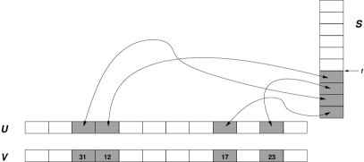
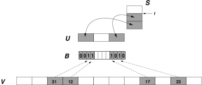
Figure 14: On the left, the classical scheme, tripling the space. On the right, our compact solution using $3n$ extra bits.

To reduce space we use, instead of array $U$ and stack $S$, a bit vector $B[1,D]$ so that $B[i]=1$ iff $V[i]$ has been initialized. This way we require only $D$ bits in addition to $V$. Of course the problem translates into initializing $B[i]\leftarrow 0$ for all $i$. We now take advantage of RAM model of computation, with word size $w\geq\lg D$.

As $B$ is stored as a contiguous sequence of bits, let us interpret this sequence as an array $B^{\prime}[1,D^{\prime}]$ of $D^{\prime}=\lceil D/w\rceil$ entries, each entry holding a computer word of $w$ bits of $B$. We can apply now the classical solution to $B^{\prime}$, so that $B^{\prime}$ can be initialized in constant time (at value $B^{\prime}[i]=0$). The extra space on top of $B^{\prime}$ is $2D^{\prime}\lg D^{\prime}\leq 2D$ bits. Together with $B^{\prime}$, the space overhead of the solution is $3D$ bits. Now, in order to determine whether $V[i]$ is initialized, we just check $B[i]$: We compute $q=\lfloor i/w\rfloor$ and $r=i~{}\textrm{mod}~{}w$ and check the bit number $r+1$ of $B^{\prime}[q+1]$. If $B^{\prime}[q+1]$ is not yet initialized, we know $B[i]=0$ and thus $V[i]$ is not yet initialized. To initialize $V[i]$ we set the $(r+1)$-th bit of $B^{\prime}[q+1]$, previously initializing $B^{\prime}[q+1]\leftarrow 0$ if needed. Fig. 14 (right) illustrates our solution.

We note that this idea can be carried out further one more level to achieve $D+o(D)$ extra bits of space, instead of $3D$.

Appendix D Proof of Correctness of Hon et al.’s Algorithm

We prove that the document listing using $o(n)$ additional bits of HSV09 is correct if we first process the left subinterval, then the block where the minimum lies, and then the right subinterval. Moreover, we show that we obtain at least one new document to list per block scanned. The need to process the recursion in this order is not clear at all in the original paper [Hon et al. (2009)].

We show by induction on the size of the current subinterval $L[i,j]$ that, if we start the procedure with the elements that already appear in $C[sp,i-1]$ marked, then we find and mark the leftmost occurrence of each distinct symbol not yet marked, spotting at least one new element per block scanned.

This is trivial for the empty interval. Now consider the minimum position in $L^{\prime}[k^{\prime}]$, which contains the leftmost occurrence of some element $C[k]$, for some $k$ within the block of $L^{\prime}[k^{\prime}]$. If $C[k]$ is already marked, it means it appears in $C[sp,i-1]$, and thus it holds $L[k]\geq sp$, and the same holds for all the values in $L[i,j]$. Thus if all the elements in the block of $L^{\prime}[k^{\prime}]$ are marked, we can safely stop the procedure.

Otherwise, before doing any marking, we recursively process the interval to the left of block $k^{\prime}$, which by inductive hypothesis marks the unique elements in that interval. Now we process the current block, finding at least the new occurrence of element $C[k]$ (which cannot appear to the left of $k^{\prime}$). Once we mark the new elements of the current block, we process the interval to the right of $k^{\prime}$, where the inductive hypothesis again holds.

The following is an example where an incorrect result is obtained if one processes the block before the left branch of the recursion.

Example D.60

Consider the color array $C=\langle 2,3,3,3,2,2,2,2,2,1,1,1\rangle$, its predecessor array $L=\langle 0,0,2,3,1,5,6,7,8,0,10,11\rangle$, and grouping factor $b=2$. Thus, we have $L^{\prime}=\langle 0,2,1,6,0,10\rangle$. If the query is for the interval $[3,12]$, it is mapped to $[2,6]$ in $L^{\prime}$. The minimum is in $L^{\prime}[5]=0$, which makes the algorithm mark colors $C[9]=2$ and $C[10]=1$, setting $V[1]\leftarrow 1$ and $V[2]\leftarrow 1$. Now we go left and consider subinterval $L^{\prime}[2,4]$, with the minimum in $L^{\prime}[3]=1$. The corresponding colors are $C[5]=2$ and $C[6]=2$. But since $V[2]=1$, both cells are already reported and the algorithm finishes in this branch of the recursion, missing color $C[3]=C[4]=3$.

Appendix E Compact Dynamic Dictionaries in Constant Worst-Case Time

We describe a dynamic structure that stores $r$ distinct keys over a universe $[1..D]$, with $t$-bit satellite data, using $O(rt)+o(r\lg D+D)$ bits. The structure supports searches and updates in constant worst-case time. This is folklore but a clear explanation is not easy to find, to the best of our knowledge.

We split the universe of keys $[1..D]$ into buckets of size $b=\lg^{2}D$. To each bucket we associate a pointer to a data structure managing the keys that fall in that bucket (this can be initialized in constant time, see Appendix C). Given a key we find its bucket in constant time with a simple division.

The structure that handles each bucket is a B-tree with arity $a=\sqrt{\lg D}$. Since the local universe of the bucket is of size $b$, the height of the B-tree is $h=O(\lg_{a}b)=O(1)$. Furthermore, the keys inside the bucket require only $O(\lg\lg D)$ bits, therefore all the keys in an internal B-tree node fit in $O(a\lg\lg D)=o(\lg D)$ bits, and thus we can find the subtree containing a key in $O(1)$ time using a precomputed table of $O(2^{o(\lg D)}b\lg b)=o(D)$ bits. Thus the B-tree searches require constant time $O(h)$.

Each B-tree is in its own memory area, which can contain up to $O(b)$ nodes, so the tree pointers require only $O(\lg\lg D)$ bits. Hence the $a$ pointers to the children can also be updated in constant time in the RAM model. Insertions and deletions of keys can, therefore, be carried out in constant worst-case time. Since each key may induce the creation of $O(h)$ nodes and also stores its satellite data, the total number of bits stored in B-tree nodes is $rt+O(ra\lg\lg D)=r(t+o(\lg D))$.

The $O(D/b)$ memory areas for the B-trees, adding up to $r(t+o(\lg D))$ bits, are stored in “extendible arrays” [Raman and Rao (2003)]. These pose an overhead of $O(rt)+o(r\lg D)+O((D/b)\lg D)$ bits and handle the accesses and grow/shrink operations on the memory areas in constant worst-case time. Since $(D/b)\lg D=o(D)$, we have the promised total space of $O(rt)+o(r\lg D+D)$ bits, and constant worst-case time for all the operations. In addition, we can maintain a linked list of the nonempty buckets to allow for $O(r)$-time traversal of the set.

Note that it is easy to carry out predecessor searches in the B-trees. By adding the structure of vEBKZ77 on the buckets, we retain the same asymptotic space and support predecessor searches and updates in time $O(\lg\lg D)$.

Appendix F Computing a Term Frequency in Compressed Space

Sad07 maintains, in addition to the global CSA, a CSA for the local suffix array $A_{d}$ of each document $T_{d}$. Since the pointers of $A_{d}$ are interspersed in $A$ in the same order, we can do the following to map a global entry $A[i]$ to the corresponding local entry $A_{d}[j]$ in its document $d$. First, compute the global text position $p=A[i]$. Then find the corresponding document $d=1+\mathsf{rank}_{1}(B,p-1)$ and its starting position in $\mathcal{T}$, $s=1+\mathsf{select}(B,d-1)$. Finally, use the inverse suffix array to map the local offset $p-s+1$ into the local suffix array of $d$, $j=A_{d}^{-1}[p-s+1]$. This is done in time $t_{\mathsf{SA}}$ with the CSAs of $A$ and $A_{d}$.

Example F.61

Let us map $A[10]$ to its local suffix array. Fig. 15 illustrates the necessary components. We compute $p=A[10]=6$ using the global CSA. Now we compute the corresponding document, $d=1+\mathsf{rank}_{1}(B,6-1)=2$, its starting position $s=1+\mathsf{select}(B,2-1)=5$, and the local offset $p-s+1=2$. Now we obtain $A_{2}^{-1}[2]=4$ with the local CSA of document $2$. Certainly, $A_{2}[4]=2$ points to the local suffix ”ma la $”, which is the same global suffix $A[10]=6$.

Figure 15: The structures for mapping global to local CSA positions.

Now imagine we know the first and last occurrence positions of a document $d$ in $C[sp,ep]$, say $i$ and $i^{\prime}$, as explained in Section 6. We use the above procedure to map them to positions $j$ and $j^{\prime}$ in $A_{d}$. Those are clearly the first and last suffixes of $A_{d}$ that start with $P$, and therefore $\mathsf{tf}(P,d)=j^{\prime}-j+1$. Since for all reasonable CSAs it holds $\sum_{d}|\mathsf{CSA}_{d}|\leq|\mathsf{CSA}|$, we have Solution 6.25.

HSV09 show how the same $\mathsf{tf}(P,d)$ can be computed, in time $O(t_{\mathsf{SA}}\,\lg n)$, if we know only the leftmost position $i$ or the rightmost position $i^{\prime}$ of the document in the range. Say it is the position $i$. We map this position to $A_{d}[j]$, and carry out an exponential search for the largest position $j^{\prime}\geq j$ such that $A_{d}[j^{\prime}]$ is mapped back to some $A[i^{\prime}]$ with $i^{\prime}\leq ep$. When we find such $j^{\prime}$, we have $\mathsf{tf}(P,d)=j^{\prime}-j+1$ (we also discover $i^{\prime}$ in the process). This mapping from $A_{d}[j^{\prime}]$ to $A[i^{\prime}]$ is the inverse of the one we described from $A[i]$ to $A_{d}[j]$, and it is computed analogously.

Appendix G Document Listing using Wavelet Trees

We start with an example of the wavelet tree structure and then show how we use it for document listing.

Example G.62

Fig. 16 displays the wavelet tree for our array $C$. Since we have $D=4$ symbols, the wavelet tree has 2 bitmap levels (plus the leaves, which are virtual and not stored). Each node shows its $C_{v}$ sequence (which is not stored) in gray and its $B_{v}$ bitmap (which is stored) in black. Each level stores $n$ bits. To recover $C[9]$ we start at the root node $v$ and read $B_{v}[9]=1$. Thus we go to the right child $u$ of $v$, where the original position $9$ becomes $\mathsf{rank}_{1}(B_{v},9)=4$ in $C_{u}$. Now $B_{u}[4]=0$, so we go to the left child of $u$ and reach the leaf of symbol $3$, thus $C[9]=3$.

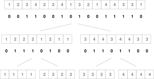
Figure 16: The wavelet tree of array $C$ in our running example. Grayed data is not represented.

GPT09 showed that the wavelet tree of $C$ allows for a completely different document listing algorithm, based on the following basic problem (also known as range selection queries).

Problem G.63 (Range Quantile)

Preprocess an array $C[1,n]$ of integers so that, given a range $[sp,ep]$ and an index $q$, we can return the $q$th smallest element in $C[sp,ep]$.

GPT09 solved this problem over a wavelet tree representation of $C$ as follows. We start at the root $v$ with interval $[sp,ep]$. We count the number of 0s in $B_{v}[sp,ep]$, with $z=\mathsf{rank}_{0}(B_{v},ep)-\mathsf{rank}_{0}(B_{v},sp-1)$. Now, if $q\leq z$, then the answer belongs to the integers handled by the left child of the root, thus we remap the interval to $sp^{\prime}=\mathsf{rank}_{0}(B_{v},sp-1)+1$ and $ep^{\prime}=\mathsf{rank}_{0}(B_{v},ep)$ and continue recursively on the left child of the root. Otherwise, we remap the interval to $sp^{\prime}=\mathsf{rank}_{1}(B_{v},sp-1)+1$ and $ep^{\prime}=\mathsf{rank}_{1}(B_{v},ep)$ and continue recursively on the right child of the root, this time looking for $q-z$ instead of $q$. When we arrive at a leaf, this is the $q$th smallest value in $C[sp,ep]$. The process takes $O(\lg D)$ time. Observe that the final $ep-sp+1$ value is the frequency of the $q$th element in the array.

Example G.64

We obtain the median of $C[5,11]$, that is, $q=4$. At the root node $v$ we count the number of $0$s in $B_{v}[5,11]$ using $\mathsf{rank}_{0}(B_{v},11)-\mathsf{rank}_{0}(B_{v},5-1)=5$. Since $5\geq 4=q$, the $q$th element of $C[5,11]$ is on the left child $u$ of $v$. Thus we descend to $u$, mapping the interval $[5,11]$ to $[\mathsf{rank}_{0}(B_{v},5-1)+1,\mathsf{rank}_{0}(B_{v},11)]=[3,7]$. Now we count the number of $0$s in $B_{u}[3,7]$ using $\mathsf{rank}_{0}(B_{u},7)-\mathsf{rank}_{0}(B_{u},3-1)=2$. Since $2<4=q$, the $q$th element of $C_{u}[3,7]$ is on the right child $w$ of $u$. Now we remap the interval $[3,7]$ to $[\mathsf{rank}_{1}(B_{u},3-1)+1,\mathsf{rank}_{1}(B_{u},7)]=[2,4]$, and since we move to the right, we set $q\leftarrow q-2=2$. Now we arrive at $w$ and, since it corresponds to the leaf of symbol $2$, we conclude that the median of $C[5,11]$ is $2$. Moreover, it occurs $4-2+1=3$ times in $C[5,11]$.

It is possible to solve the range quantile problem in time $O(\lg n/\lg\lg n)$ using $O(n\lg n)$ bits (assuming $D=O(n)$) [Brodal et al. (2011)], and this is optimal within $O(n\,\textrm{polylog}(n))$ space [Jørgensen and Larsen (2011)]. In this survey we are more interested in solutions using sublinear extra space, thus we state the wavelet tree result. It is an open problem to obtain optimal time within sublinear extra space.

Solution G.65 (Range Quantile)

[Gagie et al. (2009)] The problem can be solved in $O(\lg D)$ time on a representation of $C$ that uses $n\lg D+o(n\lg D)$ bits of space.

GPT09 use range quantile queries to solve document listing as follows. They first ask for the $q=1$st quantile of $C[sp,ep]$, thus obtaining the smallest document in the range, $d$, and its frequency, $\mathsf{tf}(P,d)$. Then they report $d$ and set $q\leftarrow q+\mathsf{tf}(P,d)$. Now they ask for the $q$th element in $C[sp,ep]$, which gives the second smallest document in the range with its frequency, and so on, until all the documents are reported. Note they do not resort to Mut02’s technique, nor they need RMQs. Moreover, they return the documents in increasing order.

While their complexity is not competitive with our previous solutions, a simplification of their method improves it [Gagie et al. (2012)]. Instead of quantile queries, just traverse all the wavelet tree paths from the root, towards left and right children, stopping either when the interval $[sp,ep]$ becomes empty, or when we arrive at a leaf handling an integer $d$, where we report document $d$ with $\mathsf{tf}(P,d)=ep-sp+1$.

Example G.66

Let us list the different values in $C[12,15]$ using range quantile queries. We ask for the $q=1$st element and get that it is $3$, which appears $2$ times. Thus we set $q\leftarrow q+2=3$ and ask for the $q=3$rd element, getting $4$, which occurs $2$ times. Thus we set $q\leftarrow q+2=5$, which is larger than our interval, so we finish.

Let us now proceed by a recursive traversal. We map the interval $C[12,15]$ to the left child of the root, obtaining $[8,7]$, which is empty, so there are no elements to report in this subtree. On the right child of the root, the interval is mapped to $[5,8]$. Now we map to its left child, obtaining $[3,4]$ at the leaf of symbol $3$, so we report $3$ with frequency $4-3+1=2$. Now we go to the right child, mapping $[5,8]$ to $[3,4]$. Now we arrive at the leaf of symbol $4$, which we also report with frequency $2$.

It is shown that the time per item output of the recursive traversal improves as more documents are listed. This results in Solution 6.27.

Appendix H Computing Document Frequency in Compressed Space

The idea is as follows [Hui (1992)]. For a node $v$ of the suffix tree, let $\mathsf{tf}(v,d)=\mathsf{tf}(str(v),d)$ for short. Thus, if $v$ is the locus of pattern $P$, it holds $\mathsf{tf}(P,d)=\mathsf{tf}(v,d)$. Now let us define $u(v)=\sum_{d,\mathsf{tf}(v,d)>0}\mathsf{tf}(v,d)-1$. It is not hard to see that $\mathsf{occ}(P,\mathcal{T})=\sum_{d,\mathsf{tf}(P,d)>0}\mathsf{tf}(P,d)=\mathsf{df}(P)+u(v)$. Thus we can easily compute $\mathsf{df}(P)=\mathsf{occ}(P,\mathcal{T})-u(v)$ in a suffix tree where $u(v)$ is computed for all the nodes.

Sad07 shows how to store this information compactly as follows. Value $u(v)$ is also the number of times the LCA of two consecutive leaves of $T_{d}$ descend from $v$ in the GST, for any $d$. Thus, if we define $h(w)$ as the number of times the LCA of two such consecutive leaves is exactly $w$, it holds $u(v)=\sum_{w~{}\mathrm{descends~{}from}~{}v}h(w)$. By storing the $h(w)$ values in preorder, we can compute $u(v)$ by adding up all the $h(w)$ values in a contiguous range. Furthermore, one can see that each pair of consecutive leaves of the same document adds 1 to some $h(w)$ value, and thus $\sum_{w}h(w)=n-D<n$. This allows us to store all the $h(w)$ values in unary, that is, concatenating $1^{h(w)}0$ to a bitmap $H[1,2n]$, so that if $p$ is the preorder of node $v$ and $s$ is the number of nodes in its subtree, we have $u(v)=\mathsf{select}_{0}(H,p+s-1)-\mathsf{select}_{0}(H,p-1)-s$. The suffix tree topology can also be represented with $O(n)$ bits so that the required operations on the suffix tree, including finding the node $v$ that covers the suffix array interval $[sp,ep]$, can be carried out in constant time [Sadakane and Navarro (2010)]. On top of any CSA, this yields Solution 7.29.

Example H.67

Fig. 17 illustrates the data structure on our example GST. We show $u$ and $h$ besides each internal node, and the bitmap representation $H$ on the bottom. For example, ”ma”, with locus $v$, occurs in $\mathsf{df}(\textsf{"ma"})=\mathsf{occ}(\textsf{"ma"},\mathcal{T})-u(v)=4-1=3$ distinct documents, where $\mathsf{occ}(\textsf{"ma"},\mathcal{T})$ is the number of leaves below $v$.

Figure 17: The data structure to compute document frequencies (only $H$ and the suffix tree topology are represented) on our running example GST.

Appendix I Optimal-Space Solution to Document Listing with Frequencies

In this section we build on the solutions of Section 10 to achieve document listing with frequencies within optimal space, obtaining Solution 10.57.

Very roughly, the idea is to use Solution 10.50, and more precisely the refinement of Solution 10.54, and ask for the top-$k$ documents in the range, for successive powers of 2 for $k$ until all the documents in the range are returned with their frequencies.

Let $c_{k}$ be the block size for tree $\rho_{k}$, for $k=1,2,4,\ldots,D$. After determining $[sp,ep]$ in $O(t_{\mathsf{search}}(m))$ time, we obtain the corresponding locus of $P$ in the successive trees $\rho_{k}$, each in constant time using an LCA operation, as explained, on the maximum $c_{k}$-aligned range $[sp^{\prime\prime},ep^{\prime\prime}]$ contained in $[sp,ep]$. We continue until the locus for some $\rho_{k}$ stores less than $k$ candidates, which means that there are less than $k$ distinct documents in the range, or when reaching $k=D$. For that $k$, the top-$k$ candidate list includes all the distinct documents in $[sp^{\prime},ep^{\prime}]$, with their frequencies. Moreover, since the locus in tree $\rho_{k/2}$ still had $k/2$ distinct elements in its $[sp^{\prime},ep^{\prime}]$ range, it holds $k/2\leq\mathsf{docc}$, and thus $k=O(\mathsf{docc})$.

To complete this precomputed set (which is actually computed on the fly with the help of $\tau_{k}$ and the sampled document array), we must traverse the $O(c_{k})$ elements of $A$ that are in $[sp,ep]\setminus[sp^{\prime},ep^{\prime}]$ and add them to the result. In those leaves we will find $(i)$ elements that already appear in $[sp^{\prime},ep^{\prime}]$, and thus their frequency has been obtained from the top-$k$ candidate list, and $(ii)$ new elements that do not appear in $[sp^{\prime},ep^{\prime}]$. This means that we do not need to store the frequencies of the $O(\sqrt{ck})$ candidates of Tsu13, but just the $O(k\lg\lg n)$ bits to correct the frequency information of the top-$k$ list. Documents found in $[sp,ep]\setminus[sp^{\prime},ep^{\prime}]$ and not in the top-$k$ list are known to have frequency zero in $[sp^{\prime},ep^{\prime}]$.

To manage the set of candidates, insert the new elements that appear, increase the counters of the elements visited, and finally collect them all for listing, we store the document identifiers in a dictionary, which offers constant worst-case time for the operations (see Appendix E).

The time is related to the block size $c_{k}=k\,\ell_{k}$. Since tree $\rho_{k}$ has $O(n/c_{k})$ nodes, the sum of the space for the lists stored in it is $O((n/c_{k})k\lg\lg n)=O((n/\ell_{k})\lg\lg n)$. Choosing $\ell_{k}=\lg k\lg^{\epsilon}n$, the space for $\rho_{k}$ is $O(n\lg\lg n/(\lg k\lg^{\epsilon}n))$ bits. Added over all the trees $\rho_{k}$ for $k=2^{i}$, this gives total space $O(n\lg\lg n/\lg^{\epsilon}n)\sum_{i=0}^{\lg D}1/i=O(n\lg\lg n\lg\lg D/\lg^{\epsilon}n)=o(n)$ bits.

References

- Aho et al. (1974) Aho, A., Hopcroft, J., and Ullman, J. 1974. The Design and Analysis of Computer Algorithms. Addison-Wesley.
- Apostolico (1985) Apostolico, A. 1985. The myriad virtues of subword trees. In Combinatorial Algorithms on Words. NATO ISI Series. Springer-Verlag, 85–96.
- Baeza-Yates and Ribeiro-Neto (2011) Baeza-Yates, R. and Ribeiro-Neto, B. 2011. Modern Information Retrieval, 2nd ed. Addison-Wesley.
- Barbay et al. (2010) Barbay, J., Gagie, T., Navarro, G., and Nekrich, Y. 2010. Alphabet partitioning for compressed rank/select and applications. In Proc. 21st Annual International Symposium on Algorithms and Computation (ISAAC). LNCS 6507. 315–326 (part II).
- Barbay et al. (2009) Barbay, J., López-Ortiz, A., Lu, T., and Salinger, A. 2009. An experimental investigation of set intersection algorithms for text searching. ACM Journal of Experimental Algorithmics 14, art. 7.
- Bartsch et al. (2011) Bartsch, A., Bunk, B., Haddad, I., Klein, J., Münch, R., Johl, T., Kärst, U., Jänsch, L., Jahn, D., and Retter, I. 2011. GeneReporter – sequence-based document retrieval and annotation. Bioinformatics 27, 7, 1034––1035.
- Bast et al. (2008) Bast, H., Mortensen, C., and Weber, I. 2008. Output-sensitive autocompletion search. Information Retrieval 11, 4, 269–286.
- Belazzougui et al. (2009) Belazzougui, D., Boldi, P., Pagh, R., and Vigna, S. 2009. Monotone minimal perfect hashing: searching a sorted table with O(1) accesses. In Proc. 20th Annual ACM-SIAM Symposium on Discrete Algorithms (SODA). 785–794.
- Belazzougui and Navarro (2011) Belazzougui, D. and Navarro, G. 2011. Alphabet-independent compressed text indexing. In Proc. 19th Annual European Symposium on Algorithms (ESA). LNCS 6942. 748–759.
- Belazzougui and Navarro (2012) Belazzougui, D. and Navarro, G. 2012. New lower and upper bounds for representing sequences. In Proc. 20th Annual European Symposium on Algorithms (ESA). LNCS 7501. 181–192.
- Belazzougui et al. (2013) Belazzougui, D., Navarro, G., and Valenzuela, D. 2013. Improved compressed indexes for full-text document retrieval. Journal of Discrete Algorithms 18, 3–13.
- Bender and Farach-Colton (2000) Bender, M. and Farach-Colton, M. 2000. The LCA problem revisited. In Proc. 4th Latin American Theoretical Informatics Symposium (LATIN). LNCS 1776. 88–94.
- Berkman and Vishkin (1993) Berkman, O. and Vishkin, U. 1993. Recursive star-tree parallel data structure. SIAM Journal on Computing 22, 2, 221–242.
- Bose et al. (2009) Bose, P., He, M., Maheshwari, A., and Morin, P. 2009. Succinct orthogonal range search structures on a grid with applications to text indexing. In Proc. 20th Symposium on Algorithms and Data Structures (WADS). LNCS 5664. 98–109.
- Brodal et al. (2011) Brodal, G., Gfeller, B., Jørgensen, A., and Sanders, P. 2011. Towards optimal range medians. Theoretical Computer Science 412, 24, 2588–2601.
- Brown (2005) Brown, F. 2005. Editorial opinion: Chemoinformatics – a ten year update. Current Opinion in Drug Discovery & Development 8, 3, 296––302.
- Büttcher et al. (2010) Büttcher, S., Clarke, C., and Cormack, G. 2010. Information Retrieval: Implementing and Evaluating Search Engines. MIT Press.
- Celikik and Bast (2009) Celikik, M. and Bast, H. 2009. Fast error-tolerant search on very large texts. In Proc. 24th ACM Symposium on Applied Computing (SAC). 1724–1731.
- Chan et al. (2012) Chan, T., Durocher, S., Larsen, K., Morrison, J., and Wilkinson, B. 2012. Linear-space data structures for range mode query in arrays. In Proc. 29th International Symposium on Theoretical Aspects of Computer Science (STACS). 290–301.
- Clark (1996) Clark, D. 1996. Compact PAT trees. Ph.D. thesis, University of Waterloo, Canada.
- Cohen and Porat (2010) Cohen, H. and Porat, E. 2010. Fast set intersection and two-patterns matching. Theoretical Computer Science 411, 40-42, 3795–3800.
- Crochemore and Rytter (2002) Crochemore, M. and Rytter, W. 2002. Jewels of Stringology. World Scientific.
- Croft et al. (2009) Croft, B., Metzler, D., and Strohman, T. 2009. Search Engines: Information Retrieval in Practice. Pearson Education.
- Culpepper et al. (2010) Culpepper, S., Navarro, G., Puglisi, S., and Turpin, A. 2010. Top-k ranked document search in general text databases. In Proc. 18th Annual European Symposium on Algorithms (ESA). LNCS 6347. 194–205 (part II).
- Culpepper et al. (2012) Culpepper, S., Petri, M., and Scholer, F. 2012. Efficient in-memory top-k document retrieval. In Proc. 35th International ACM Conference on Research and Development in Information Retrieval (SIGIR). 225–234.
- Farach (1997) Farach, M. 1997. Optimal suffix tree construction with large alphabets. In Proc. 38th IEEE Symposium on Foundations of Computer Science (FOCS). 137–143.
- Fariña et al. (2012) Fariña, A., Brisaboa, N., Navarro, G., Claude, F., Places, A., and Rodríguez, E. 2012. Word-based self-indexes for natural language text. ACM Transactions on Information Systems 30, 1, art. 1.
- Ferrada and Navarro (2013) Ferrada, H. and Navarro, G. 2013. A Lempel-Ziv compressed structure for document listing. In Proc. 20th International Symposium on String Processing and Information Retrieval (SPIRE). LNCS 8214. 116–128.
- Ferragina et al. (2009) Ferragina, P., González, R., Navarro, G., and Venturini, R. 2009. Compressed text indexes: From theory to practice. ACM Journal of Experimental Algorithmics 13, art. 12.
- Ferragina et al. (2003) Ferragina, P., Koudas, N., Muthukrishnan, S., and Srivastava, D. 2003. Two-dimensional substring indexing. Journal of Computer and System Sciences 66, 4, 763–774.
- Fischer et al. (2012) Fischer, J., Gagie, T., Kopelowitz, T., Lewenstein, M., Mäkinen, V., Salmela, L., and Välimäki, N. 2012. Forbidden patterns. In Proc. 10th Latin American Symposium on Theoretical Informatics (LATIN). LNCS 7256. 327–337.
- Fischer and Heun (2011) Fischer, J. and Heun, V. 2011. Space-efficient preprocessing schemes for range minimum queries on static arrays. SIAM Journal on Computing 40, 2, 465–492.
- Gabow et al. (1984) Gabow, H., Bentley, J., and Tarjan, R. 1984. Scaling and related techniques for geometry problems. In Proc. 16th ACM Symposium on Theory of Computing (STOC). 135–143.
- Gagie et al. (2013) Gagie, T., Kärkkäinen, J., Navarro, G., and Puglisi, S. 2013. Colored range queries and document retrieval. Theoretical Computer Science 483, 36–50.
- Gagie et al. (2012) Gagie, T., Navarro, G., and Puglisi, S. J. 2012. New algorithms on wavelet trees and applications to information retrieval. Theoretical Computer Science 426-427, 25–41.
- Gagie et al. (2009) Gagie, T., Puglisi, S. J., and Turpin, A. 2009. Range quantile queries: Another virtue of wavelet trees. In Proc. 16th International Symposium on String Processing and Information Retrieval (SPIRE). LNCS 5721. 1–6.
- Golynski et al. (2006) Golynski, A., Munro, I., and Rao, S. 2006. Rank/select operations on large alphabets: a tool for text indexing. In Proc. 17th Annual ACM-SIAM Symposium on Discrete Algorithms (SODA). 368–373.
- Gonnet et al. (1992) Gonnet, G., Baeza-Yates, R., and Snider, T. 1992. Information Retrieval: Data Structures and Algorithms. Prentice-Hall, Chapter 3: New indices for text: PAT trees and PAT arrays, 66–82.
- González and Navarro (2007) González, R. and Navarro, G. 2007. Compressed text indexes with fast locate. In Proc. 18th Annual Symposium on Combinatorial Pattern Matching (CPM). LNCS 4580. 216–227.
- Greve et al. (2010) Greve, M., Jørgensen, A. G., Larsen, K. D., and Truelsen, J. 2010. Cell probe lower bounds and approximations for range mode. In Proc. 37th International Colloquim on Automata, Languages and Programming (ICALP). 605–616.
- Grossi et al. (2003) Grossi, R., Gupta, A., and Vitter, J. 2003. High-order entropy-compressed text indexes. In Proc. 14th Annual ACM-SIAM Symposium on Discrete Algorithms (SODA). 841–850.
- Grossi et al. (2010) Grossi, R., Orlandi, A., and Raman, R. 2010. Optimal trade-offs for succinct string indexes. In Proc. 37th International Colloquim on Automata, Languages and Programming (ICALP). 678–689.
- Gupta et al. (1995) Gupta, P., Janardan, R., and Smid, M. 1995. Further results on generalized intersection searching problems: Counting, reporting, and dynamization. Journal of Algorithms 19, 2, 282–317.
- Gusfield (1997) Gusfield, D. 1997. Algorithms on Strings, Trees and Sequences: Computer Science and Computational Biology. Cambridge University Press.
- Harel and Tarjan (1984) Harel, D. and Tarjan, R. 1984. Fast algorithms for finding nearest common ancestors. SIAM Journal on Computing 13, 2, 338–355.
- Heaps (1978) Heaps, H. 1978. Information Retrieval: Theoretical and Computational Aspects. Academic Press.
- Hon et al. (2010a) Hon, W.-K., Patil, M., Shah, R., and Wu, S.-B. 2010a. Efficient index for retrieving top-k most frequent documents. Journal of Discrete Algorithms 8, 4, 402–417.
- Hon et al. (2012a) Hon, W.-K., Shah, R., and Thankachan, S. 2012a. Towards an optimal space-and-query-time index for top-k document retrieval. In Proc. 23rd Annual Symposium on Combinatorial Pattern Matching (CPM). LNCS 7354. 173–184.
- Hon et al. (2010b) Hon, W.-K., Shah, R., Thankachan, S., and Vitter, J. 2010b. String retrieval for multi-pattern queries. In Proc. 17th International Symposium on String Processing and Information Retrieval (SPIRE). LNCS 6393. 55–66.
- Hon et al. (2012b) Hon, W.-K., Shah, R., Thankachan, S., and Vitter, J. 2012b. Document listing for queries with excluded pattern. In Proc. 23rd Annual Symposium on Combinatorial Pattern Matching (CPM). LNCS 7354. 185–195.
- Hon et al. (2013) Hon, W.-K., Shah, R., Thankachan, S., and Vitter, J. 2013. Faster compressed top-k document retrieval. In Proc. 23rd Data Compression Conference (DCC). 341–350.
- Hon et al. (2009) Hon, W.-K., Shah, R., and Vitter, J. 2009. Space-efficient framework for top- string retrieval problems. In Proc. 50th IEEE Annual Symposium on Foundations of Computer Science (FOCS). 713–722.
- Hon et al. (2010c) Hon, W.-K., Shah, R., and Vitter, J. S. 2010c. Compression, indexing, and retrieval for massive string data. In Proc. 21st Annual Symposium on Combinatorial Pattern Matching (CPM). LNCS 6129. 260–274.
- Hsu and Ottaviano (2013) Hsu, P. and Ottaviano, G. 2013. Space-efficient data structures for top-k completion. In Proc. 22nd World Wide Web Conference (WWW). 583–594.
- Hui (1992) Hui, L. 1992. Color set size problem with applications to string matching. In Proc. 3rd Annual Symposium on Combinatorial Pattern Matching (CPM). LNCS 644. 227––240.
- Janardan and Lopez (1993) Janardan, R. and Lopez, M. 1993. Generalized intersection searching problems. International Journal of Computational Geometry Applications 3, 1, 39–69.
- Jørgensen and Larsen (2011) Jørgensen, A. and Larsen, K. 2011. Range selection and median: Tight cell probe lower bounds and adaptive data structures. In Proc. 22nd Symposium on Discrete Algorithms (SODA). 805–813.
- Kärkkäinen et al. (2006) Kärkkäinen, J., Sanders, P., and Burkhardt, S. 2006. Linear work suffix array construction. Journal of the ACM 53, 6, 918–936.