Magnetic fields around evolved stars: further observations of H₂O maser polarization

Abstract

Context. A low- or intermediate-mass star is believed to maintain a spherical shape throughout the evolution from the main sequence to the Asymptotic Giant Branch (AGB) phase. However, many post-AGB objects and planetary nebulae exhibit non-spherical symmetry. Several candidates have been suggested as factors that can play a role in this change of morphology, but the problem is still not well understood. Magnetic fields are one of these possible agents.

Aims. We aim to detect the magnetic field and infer its properties around four AGB stars using H₂O maser observations. The sample we observed consists of the following sources: the semi-regular variable RT Vir, and the Mira variables AP Lyn, IK Tau, and IRC$+$60370.

Methods. We observed the 6${}_{1,6}-$5_2,3 H₂O maser rotational transition in full-polarization mode to determine its linear and circular polarization. Based on the Zeeman effect, one can infer the properties of the magnetic field from the maser polarization analysis.

Results. We detected a total of 238 maser features in three of the four observed sources. No masers were found toward AP Lyn. The observed masers are all located between 2.4 and 53.0 AU from the stars. Linear and circular polarization was found in 18 and 11 maser features, respectively.

Conclusions. We more than doubled the number of AGB stars in which a magnetic field has been detected from H₂O maser polarization. Our results confirm the presence of fields around IK Tau, RT Vir, and IRC$+$60370. The strength of the field along the line of sight is found to be between 47 and 331 mG in the H₂O maser region. Extrapolating this result to the surface of the stars, assuming a toroidal field ($\propto$ r^-1), we find magnetic fields of 0.3$-$6.9 G on the stellar surfaces. If, instead of a toroidal field, we assume a poloidal field ($\propto$ r^-2), then the extrapolated magnetic field strength on the stellar surfaces are in the range between 2.2 and $\sim$115 G. Finally, if a dipole field ($\propto$ r^-3) is assumed, the field strength on the surface of the star is found to be between 15.8 and $\sim$1945 G. The magnetic energy of our sources is higher than the thermal and kinetic energy in the H₂O maser region of this class of objects. This leads us to conclude that, indeed, magnetic fields probably play an important role in shaping the outflows of evolved stars.

1 Introduction

Low- and intermediate-mass stars (0.8$-$8 M_⊙) are believed to maintain their sphericity until the asymptotic giant branch (AGB) phase. Even though some AGB stars are slightly elliptical (e.g., Reid & Menten 2007; Castro-Carrizo 2010), many planetary nebulae (PNe) do not present any spherical symmetry. How an almost-spherical AGB star gives rise to a non-spherical PN is still an open question. A companion to the star (binary system or a massive planet), disk interaction, the influence of magnetic fields, or a combination of these agents are candidates to explain this phenomenon (Balick & Frank 2002; Frank et al. 2007; Nordhaus et al. 2007,  and references therein).

Magneto-hydrodynamic (MHD) simulations show that the magnetic field can be an important agent in shaping post-AGBs and PNe (e.g., García-Segura et al. 1999, 2005; García-Díaz et al. 2008; Dennis et al. 2009). Moreover, recent observations support the presence of magnetic fields around AGB and post-AGB stars (e.g., Amiri et al. 2011; Pérez-Sánchez et al. 2011; Leal-Ferreira et al. 2012; Vlemmings et al. 2012). However, the sample of low and intermediate mass evolved stars around which magnetic fields have been measured is still small. So far, detections of magnetic field from H₂O maser polarization were reported around two AGB stars only; U Her and U Ori (Vlemmings et al. 2002, 2005). Also, the morphology and strength of the magnetic field as a function of radial distance throughout the circumstellar envelope is still unclear. Observations of different magnetic field tracers are needed to constrain the field dependence on the radial distance from the star and, therefore, improve future MHD simulations.

Different maser species can provide information about different regions around these objects. While SiO masers are expected to be found within the extended atmosphere of the star (between the photosphere and the dust formation zone), OH masers are detected much further out ($\sim$65$-$650 AU). The H₂O masers emit at an intermediate distance to the star, between the SiO and OH maser regions. The distance of the H₂O masers from the star is expected to lie within a few to less than a hundred AU (e.g., Cohen 1987; Bowers et al. 1989; Elitzur 1992).

The present work aims to enlarge the number of magnetic field detections around low- and intermediate-mass evolved stars. We imaged five sources of this class using very-long-baseline interferometry (VLBI), in full-polarization mode, with the goal of detecting H₂O masers around them. As a result of Zeeman splitting (Zeeman 1897), we can measure the magnetic field signature on maser lines by investigating the polarized emission of the masers (e.g., Vlemmings et al. 2001, 2006).

Our sample is composed of the pre-PN OH231.8$+$4.2, the semi-regular variable RT Vir, and the Mira variables AP Lyn, IK Tau, and IRC$+$60370. We presented the results of OH231.8$+$4.2 in Leal-Ferreira et al. (2012). The analysis of the four remaining sources is presented in the present paper. Single-dish SiO maser observations in full-polarization mode have been previously reported by Herpin et al. (2006) for RT Vir, AP Lyn, and IK Tau. Their results show a magnetic field of 0 $\leq$ $B_{||}$[G] $\leq$ 5.6 in RT Vir, 0.9 $\leq$ $B_{||}$[G] $\leq$ 5.6 in AP Lyn, and 1.9 $\leq$ $B_{||}$[G] $\leq$ 6.0 in IK Tau. The AGB star RT Vir also shows strong circular polarization in single dish OH maser observations, indicating a strong global magnetic field (Szymczak et al. 2001). We did not find any literature reports concerning the magnetic field for IRC$+$60370 in the SiO maser region, nor for AP Lyn, IK Tau, and IRC$+$60370 in the OH maser region.

This paper is structured as follows: in Sect. 2, we describe the observations, data reduction, and calibration; in Sect. 3, we present the results; in Sect. 4, we discuss the results and, in Sect. 5, we conclude the analysis.

2 Observations and data reduction

We used the NRAO Very Long Baseline Array (VLBA) to observe the H₂O 6${}_{1,6}-$5_2,3 rotational maser transition at a rest frequency toward 22.235081 GHz of the stars in our sample. In each observing run, we used two baseband filters and performed separate lower (Low) and higher (High) resolution correlation passes. The first was performed in full-polarization mode and the second in dual-polarization mode. We show the characteristics of the Low and High correlation passes in Table 1 and the individual observation details of each source in Table 2.

Table 1: Low- and high-resolution correlation passes

Label	Nchans	BW	$\triangle v$	PolMode
		(MHz)	(km/s)
Low	128	1.0	0.104	Full (LL,RR,LR,RL)
High	512	1.0	0.026	Dual (RR,LL)

Correlation parameters for the low- and high-resolution correlation passes. Description of Cols. 1 to 5: The label of the observed data $-$ low- (Low) and high- (High) resolution $-$ (Label), the number of channels (N_chans), the bandwidth (BW), the channel width ($\triangle v$), and the polarization mode (PolMode).

Table 2: Source observation details

Code	Source	Class	Vlsr(IF1)	Vlsr(IF2)	Beam	RA0	Dec0	Date
			(km/s)	(km/s)	(mas)	(J2000)	(J2000)	(mm/dd/yy)
BV067A*	OH231.8$+$4.2	pre-Planetary Nebula	$+$44.0	$+$26.0	1.7$\times$0.9	07h42m16.93s	–14∘42’50”.2	03/01/09
BV067B	AP Lyn	Mira variable	–19.5	–32.5	–	06h34m34.88s	$+$60∘56’33”.2	03/15/09
BV067C	IK Tau	Mira variable	$+$42.5	$+$29.5	1.2$\times$0.5	03h53m28.84s	$+$11∘24’22”.6	02/20/09
BV067D	RT Vir	Semi-regular variable	$+$25.5	$+$12.5	1.2$\times$0.9	13h02m37.98s	$+$05∘11’08”.4	03/15/09
BV067E	IRC$+$60370	Mira variable	–44.5	–57.5	0.8$\times$0.5	22h49m58.88s	$+$60∘17’56”.7	03/05/09
*Presented in Leal-Ferreira et al. (2012)

From left to right: The project code (Code), the name of the source (Source), the nature of the source (Class), the velocity center position of each of the 2 filters (v_lsr), the PSF beam size (Beam), the center coordinates of the observations (RA₀ and Dec₀), and the starting observation date (Date).

We observed different calibrators for each target. Each calibrator was observed during the same run as its corresponding target. For the calibration of RT Vir, we used 3C84 (bandpass, delay, polarization leakage, and amplitude). To calibrate IK Tau, we used J0238$+$16 (bandpass, delay, and amplitude) and 3C84 (polarization leakage). To calibrate IRC$+$60370, we used BLLAC (bandpass, delay, polarization leakage, polarization absolute angle, and amplitude). Unfortunately, no good absolute polarization angle calibrator were available for RT Vir and IK Tau, making it impossible to determine the absolute direction of the linear polarization vectors (also referred to as electric vector position angle; EVPA). However, the relative EVPA angles for individual polarized components within RT Vir are still correct (no linear polarization was detected for IK Tau). To determine the absolute EVPA of IRC$+$60370, we created a map of BLLAC and compared the direction of the measured EVPA with that reported in the VLA/VLBA polarization calibration database. Our IRC$+$60370 observation was carried out between the calibration observations of February 21 and March 19, 2009 in that database, where the polarization angle of BLLAC changed from 25.7^∘ to 26.0^∘. We thus adopted a reference angle of 25.8^∘ to obtain the absolute EVPA.

After an initial analysis of the raw data, we did not detect any maser emission around AP Lyn and so did not proceed with further calibration of this data set. For the other three targets, we used the Astronomical Image Processing Software Package (AIPS) and followed the data reduction procedure documented by Kemball et al. (1995) to perform all the necessary calibration steps. This included using the AIPS task SPCAL to determine polarization leakage parameters using a strong maser feature.

After the data were properly calibrated, we used the low-resolution data to create the image cubes for the Stokes parameters $I$, $Q$, $U$, and $V$. The $Q$ and $U$ cubes were used to generate the linear polarization intensity ($P=\sqrt[]{Q^{2}+U^{2}}$) cubes and the EVPA cubes. The noise level measured on the emission-free channels of the low-resolution data cubes is between $\sim$2 mJy and $\sim$6 mJy. The high-resolution data were used to create the data cubes of the Stokes parameters $I$ and $V$, from which the circular polarization could be inferred. The noise level measured from the emission-free channels of the high-resolution data cubes is between $\sim$5 mJy and $\sim$11 mJy.

The detection of the maser spots was done by using the program maser finder, as described by Surcis et al. (2011). We defined a maser feature to be successfully detected when maser spots located at similar spatial positions (within the beam size) survive the signal-to-noise ratio cutoff we adopted (8 $\sigma$) in at least three consecutive channels. The position of the maser feature was taken to be the position of the maser spot in the channel with the peak emission of the feature (see e.g., Richards et al. 2011).

3 Results

We found 85 maser features around IK Tau, 91 toward RT Vir, and 62 around IRC$+$60370. The maser identification and properties are shown in Table LABEL:results. In Fig. 1 we show the spatial distribution of the maser components (depicted as circles). The size of the circles is proportional to the maser flux densities, and they are colored according to velocity. The black cross indicates the stellar position determined in Sect. 4.3.

Positive linear polarization detection is reported when successfully found in at least two consecutive channels. The linear polarization percentage ($P_{L}$) quoted in Table LABEL:results is the $P_{L}$ measured in the brightest channel of the feature. The $P_{L}$ error is given by the rms of the $P$ spectrum on the feature spatial position, scaled by the intensity peak. The $EVPA$ error was determined using the expression $\sigma_{EVPA}=0.5\leavevmode\nobreak\ \sigma_{P}/P\times 180^{\circ}/\pi$ (Wardle & Kronberg 1974). The linear polarization results are enumerated in Cols. 8 ($P_{L}$) and 9 ($EVPA$) of Table LABEL:results. In Fig. 1, the black vectors show the $EVPA$ of the features in which linear polarization is present. The length of the vectors is proportional to the polarization percentage.

To measure the circular polarization, we used the $I$ and $V$ spectra to perform the Zeeman analysis described by Vlemmings et al. (2002). In this approach, the fraction of circular polarization, $P_{V}$, is given by

$$P_{V} = (V_{max}\leavevmode\nobreak\ -\leavevmode\nobreak\ V_{min})/I_{max}$$ (1)

$$= 2\leavevmode\nobreak\ \times A_{F-F^{\prime}}\leavevmode\nobreak\ \times B_{||}[Gauss]/\Delta v_{L}[km/s],$$

where $V_{max}$ and $V_{min}$ are the maximum and minimum of the model fitted to the $V$ spectrum, and $I_{max}$ is the peak flux of the emission. The variable $A_{F-F^{\prime}}$ is the Zeeman splitting coefficient. Its exact value depends on the relative contribution of each hyperfine component of the H₂O 6${}_{1,6}-$5_2,3 rotational maser transition. We adopted the value $A_{F-F^{\prime}}$ = 0.018, which is the typical value found by Vlemmings et al. (2002). The projected magnetic field strength along the line of sight is given by $B_{||}$ and $\Delta v_{L}$ is the full-width half-maximum of the $I$ spectrum. Although the non-LTE analysis in Vlemmings et al. (2002) has shown that the circular polarization spectra are not necessarily strictly proportional to $dI/d\nu$, using $A_{F-F^{\prime}}$, determined by a non-LTE fit, introduces a fractional error of less than $\sim$20$\%$ when using Eq. 1. We report circular polarization detection when the magnetic field strength given by the model fit is $\geq$ 3$\sigma$. The reported errors are based on the single channel rms using Eq. 1 (see Leal-Ferreira et al. 2012, Sect. 3.3, for further discussion). We list the $P_{V}$ and $B_{||}$ results in Cols. 10 and 11 of Table LABEL:results, where the positive sign on $B_{||}$ indicates that the direction of the magnetic field along the line of sight is away from the observer, while the negative sign corresponds to a direction towards the observer. In Figs. 2 and 3, we present the $I$ and $V$ spectra and the model fit of $V$ spectra for those features in which we detect circular polarization.

3.1 IK Tau

We observed a total of 642 H₂O maser spots toward IK Tau. Of these, 525 spots survived the multi-channel criteria and comprise 85 maser features around this source. In Figs. 1.I, we present the spatial distribution of these 85 maser features. In Fig. 1.II and 1.III, we zoom in on the two areas indicated in Fig. 1.I.

We did not find linear polarization in any maser feature around IK Tau. However, circular polarization was detected in three features around this source: IK.20, IK.69, and IK.84 (see Table LABEL:results). The magnetic field strength along the line of sight given by the model fits are: $-$147$\pm$15 mG, $-$96$\pm$31 mG, and $+$215$\pm$56 mG, respectively. These features are identified in Fig. 1 labeled according to their field strengths.

Figure 1: Maps of the maser features detected toward RT Vir, IK Tau, and IRC$+$60370. The size of the circles is proportional to the maser flux densities, and their colors show the velocity scale. The black crosses indicate the stellar positions (see Sect. 4.3). The black lines indicate the EVPA (for RT Vir, they could not be calibrated in terms of absolute EVPA), and their lengths are proportional to the fractional linear polarization. The magnetic field strength along the line of sight are also shown for the features in which we detected circular polarization. The x-axis is the projected offset on the plane of the sky in the direction of right ascension. The y-axis is the declination offset. The offsets are with respect to the reference maser.

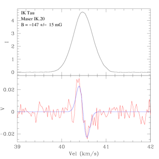
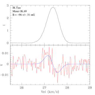
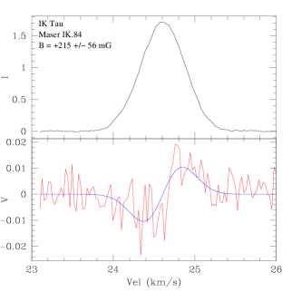
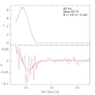
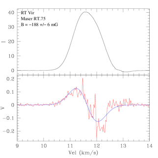
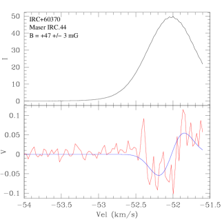
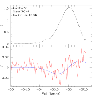
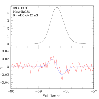
Figure 2: Plots of Stokes $I$ (top; black line) and $V$ (bottom; red line) spectra of all maser features in which we detected circular polarization. The blue lines show the best model fit to each $V$ spectrum. The source, the maser identification, and the magnetic field strength along the line of sight given by the fit are presented in top-left corner of each plot. The x-axis shows $V_{LSR}$ in km/s and the y-axis the intensity in Jy/beam.

3.2 RT Vir

We observed 830 H₂O maser spots toward RT Vir in total. Of these, 671 spots comprise 91 maser features around this source. In Fig. 1.IV, we present the spatial distribution of these 91 maser features and in Fig. 1.V we show an enlargement of the area indicated in Fig. 1.IV.

We detected linear polarization in nine features toward RT Vir: RT.31, RT.34, RT.67, RT.68, RT.70, RT.72, RT.73, RT.75, and RT.90 (see Table LABEL:results). Unfortunately, no good polarization calibrator was available, making it impossible to determine the absolute direction of the polarization vectors (the relative $EVPA$ between components is still correct).

The distribution of $EVPA$ among the nine features clearly distinguishes two groups of masers. Six features, located within projected right ascension offset $-$40 $\lesssim\alpha_{off}\lesssim$ 0 mas and declination offset $-$10 $\lesssim\delta_{off}\lesssim$ 30 mas (Fig. 1.V) have $EVPA$ between $-$38^∘ and $-$59^∘. Another group of features, located within 25 $\lesssim\alpha_{off}\lesssim$ 35 mas and $-$15 $\lesssim\delta_{off}\lesssim$ 5 mas (Fig. 1.V), also has a small $EVPA$ dispersion ($+$38^∘ $\leq$ $EVPA$ $\leq$ $+$64^∘).

Circular polarization was found in three features around RT Vir: RT.70, RT.75, and RT.90. From the fit of the $V$ spectra, we inferred magnetic field strengths along the line of sight of $-$143$\pm$12 mG and $-$188$\pm$6 mG in RT.70 and RT.75, respectively. We note, however, that the model fit of RT.70 does not superimpose the whole S-shape structure of its V spectrum. This is a consequence of the strong emission that peaks at 11.7 km/s (RT.75). Because of this strong emission, a higher noise is present in the spectra around 11.7 km/s. Therefore, we truncated the RT.70 spectrum at velocity values lower than 12.6 km/s to minimize the impact of this noise on the fit. However, even with this truncation, a high noise is still present in part of the V spectrum and so the results from the model fit of RT.70 should be taken with caution.

The shape of the $V$ spectrum of RT.90 suggests blended emission. There are many free parameters to be taken into account in fitting emission of blended features. Consequently, any attempt to obtain a magnetic field strength from RT.90 will not generate a solution that is unique or robust. However, it is important to emphasize that the shape of its $V$ spectrum clearly indicates the presence of a magnetic field. As an example, we created a possible fit for this feature. The solution we found for this fit gives a magnetic field of $-$84 mG for the slightly more blue-shifted emission and $+$63 mG for the slightly more red-shifted feature. The features themselves are separated by approximately 0.2 km/s and have widths of 0.38 and 0.4 km/s. We present this possible fit in Fig. 3.

In Fig. 1.V, RT.70, RT.75, and RT.90 are labeled with the magnetic field strength along the line of sight obtained from the model fits shown in Figs. 2 and 3.

Figure 3: Spectra I and V (black curves) of RT.90. The dashed lines show the fit of the individual blended features. In red, we show a fit for I and V.

3.3 IRC$+$60370

We observed 658 H₂O maser spots in IRC$+$60370 in total. Of these, 634 spots comprise 62 maser features around this source. In Fig. 1.VI, we present the spatial distribution of these 62 maser features and in Fig. 1.VII and 1.VIII we show an enlargement of the areas indicated in Fig. 1.VI.

We detected linear polarization in nine features toward IRC$+$60370. These nine features are concentrated in two small projected regions, with areas of $\sim$2 mas² each. Six of them are located within $-$2 $\lesssim\alpha_{off}\lesssim$ 0 mas and $-$1 $\lesssim\delta_{off}\lesssim$ 3 mas (Fig. 1.VII; Zoom A). The other three features with linear polarization detection are located within 27 $\lesssim\alpha_{off}\lesssim$ 29 mas and 6 $\lesssim\delta_{off}\lesssim$ 8 mas (Fig. 1.VIII; Zoom B). The EVPA of the masers in Zoom A vary from $-$97^∘ to $-$39^∘, while the EVPA of the masers in Zoom B are between $-$74^∘ and $-$132^∘.

Circular polarization was found in five features around IRC$+$60370: IRC.44, IRC.45, IRC.47, IRC.48, and IRC.58. From the model fit to the V spectra, we measured magnetic field strengths along the line of sight of $+$47$\pm$3 mG, $+$266$\pm$30 mG, $+$331$\pm$82 mG, $+$273$\pm$18 mG, and $-$130$\pm$22 mG, respectively. We note that, once more, the model fit of several features does not superimpose the full expected S-shape of the V spectra. For this source three factors contributed to this: (i) the limit of the observed spectral range, (ii) features with similar spatial and spectral position, and (iii) the increase in the noise near -52 km/s, due to the strong feature IRC.44. Therefore, the results given by the fit to IRC.44, IRC.45, IRC.47, and IRC.48 should also be taken with caution. In Fig. 1.VII, the five features with circular polarization detection are labeled with the magnetic field strength along the line of sight that we obtained from the model fits shown in Fig. 2.

4 Discussion

4.1 Non-detection toward AP Lyn

Several H₂O masers toward AP Lyn have been detected before (e.g., Imai et al. 1997; Migenes et al. 1999; Colomer et al. 2000; Sudou et al. 2002; Shintani et al. 2008; Kim et al. 2010). Shintani et al. (2008) monitored this and other sources from 2003 to 2006, using the Iriki 20 m telescope of the VLBI Exploration of Radio Astrometry (VERA). They reported a high flux variation, and fit a maser light curve for Ap Lyn. The peak flux of the H₂O masers reported in the other works vary from $\sim$6 Jy (observed with the VLBA in 1996; Migenes et al. 1999) up to $\sim$120 Jy (observed with the Kashima-Nobeyama Interferometer in 1992; Sudou et al. 2002). Conservatively, we suggest an upper limit of 1 Jy for the flux density of our non-detection (in the raw data).

Richards et al. (2012) give a detailed discussion of the possible causes of H₂O maser variability. They point out that a correlation of the infrared light curve and maser variability can exist. Also, they disagree with previous papers (e.g., Shintani et al. 2008) stating that no systematic relationship between maser brighness and the optical phase was found at the times of their observations.

4.2 Spatial distribution of the masers

The spatial distribution of the features around IK Tau shows a clear correlation between velocity and position. While masers with higher velocities (red circles) are concentrated in the west and southwest, the features with lower velocity (blue circles) appear, mostly, in the east and northeast (Fig. 1.I). This behavior is also reported by Bains et al. (2003). They suggest that the shell of IK Tau has an equatorial density enhancement. The brightest masers would lie in an oblate spheroid and the plane of the equator would have an inclination angle $i^{\prime}$ with the line of sight (45${}^{\circ}\lesssim i^{\prime}\lesssim$ 90^∘). The eastern end of the polar axis would then be approaching us, explaining the east-west velocity segregation. This model also explains why the IK Tau observations made more than 10 years apart show a persistent east-west offset between moderately red- and blue-shifted emission, although individual masers do not survive for more than $\sim$1.5 years. Our IK Tau data were observed in 2009, almost 15 years later than the observations reported by Bains et al. (2003), and 24 years after the observations reported by Yates & Cohen (1994).

Bains et al. (2003) also observed a similar east-west velocity offset in RT Vir. Our data do not show a clear correlation between velocity and position for this source (Fig. 1.I), but a moderate enhanced concentration of red-shifted features in the east is present, while the bluer features are concentrated in the center of the plot. This is different from the east-west relation seen in Fig. 6 of Bains et al. (2003). In their figure, the red-shifted masers are located on the western side, and the blue-shifted features are concentrated on the eastern side.

An individual H₂O maser has its life time estimated to be less than 1–2 years. Multi-epoch imaging of 22 GHz H₂O masers often shows major changes in the maser distribution over the years (e.g., Richards et al. 2012). IK Tau is, therefore, an exception to this behavior.

4.3 Stellar Position

Some of the analysis discussed in this paper requires information concerning the stellar position in relation to the observed masers (Sects. 4.4 and 4.5). However, the absolute stellar position is not known for our observations. So to infer the stellar position, we used the shell-fitting method (Yates 1993; Bains et al. 2003). This method assumes a distribution of masers on a tridimensional sphere, with the star located in its center. All masers in a velocity range determined by

$$V_{star}\pm i(\Delta V_{LSR}/n)$$ (2)

are identified, where $V_{star}$ is the velocity of the star, $\Delta V_{LSR}$ the total maser velocity range, and $n$ is a number taken here to be equal to 8. We choose that value to restrict the selection of the masers to lie within a small velocity range. The constant $i$ sets which ring(s) along the line of sight is considered. If $i$ is equal to 1, then a ring at the same line of sight velocity as the star is taken. If $i$ is bigger than 1, then one ring in front and one behind of the star are considered. Once the masers are selected, the central position of the features is assumed to be the stellar position. We emphasize that the more asymmetric the maser distribution, the larger the uncertainty of this method.

For each object, we varied the value of $i$, obtaining different locations for the stellar position. An additional position was calculated by taking the center point of all the observed masers. We assumed the stellar position to be the mean location of the different positions we obtained by using different values of $i$, and by using the center point of all the observed masers. In Table 3 we show the stellar position we calculated for each value of $i$ and the mean result.

Table 3: Stellar position

	IK Tau	RT Vir	IRC$+$60370
	$\alpha$, $\delta$ (mas)	$\alpha$, $\delta$ (mas)	$\alpha$, $\delta$ (mas)
$i$=1	–	$\alpha$ = +04.51	$\alpha$ = +07.44
	–	$\delta$ = –13.83	$\delta$ = +03.57
$i$=2	$\alpha$ = +07.43	–	$\alpha$ = +14.49
	$\delta$ = +03.09	–	$\delta$ = +03.61
$i$=3	$\alpha$ = +28.58	–	$\alpha$ = +11.17
	$\delta$ = –05.38	–	$\delta$ = +01.99
All Features	$\alpha$ = +10.41	$\alpha$ = +10.69	$\alpha$ = +10.92
	$\delta$ = +02.36	$\delta$ = –15.32	$\delta$ = +02.68
Mean Position	$\alpha$ = +15.47	$\alpha$ = +07.60	$\alpha$ = +11.01
	$\delta$ = +00.02	$\delta$ = –14.58	$\delta$ = +02.96

Position of the star, relative to the reference maser, for different values of $i$. The positions we obtained as the centroid of all the observed maser features are also shown. Finally, the mean result is reported at the bottom of the table. Columns 2 to 4 show the stellar position of IK Tau, RT Vir, and IRC$+$60370.

4.4 Distance of the masers to the star

In Fig. 4 we show, for each source, a plot of the velocity of the features versus their projected angular offsets from the star ($\theta_{off}$; see Sect. 4.3 for the determination of the stellar position). For each source, two parabolas are fitted to the velocity-offset positions. These fits are shown by the dotted lines in the figures. In the fitting process, made by eye, the area between the parabolas which contains all masers is minimized. The parabolas obey the relation

$$\theta_{off} = \frac{R}{V_{shell}}\times(V_{shell}^{2}-(V_{LSR}-V_{star})^{2})^{1/2},$$ (3)

where $R$ is the distance to the star, $V_{shell}$ the expanding velocity of the masers, and $V_{star}$ the velocity of the star.

Assuming that the masers are located in a spherical shell around the star, it is possible to determine the internal ($R_{i}$) and external ($R_{o}$) radius of this shell from the internal and external parabola fits, and their corresponding expansion velocities ($v_{i}$ and $v_{o}$). The values we adopted for $V_{star}$, the distance to the source, their respective references, and the fit parameters ($v_{i}$, $v_{o}$, $R_{i}$, $R_{o}$) are shown in Table 4.

Bains et al. (2003) and Richards et al. (2011) also investigated the kinematics of IK Tau and RT Vir and found similar results for $v_{i}$, $v_{o}$, $R_{i}$, and $R_{o}$. To illustrate the comparison with our results, we reproduce the fits from Bains et al. (2003) for IK Tau and RT Vir in our Fig. 4. Those authors present two alternative solutions for the internal fit to IK Tau. We choose to show only the one with the larger radius here. Their fits are shown in Fig. 4 by the dashed lines. We note that there is a big disagreement between the external fits from Bains et al. (2003) and ours. This is probably because our observations with the VLBA resolve out more diffuse emissions, due to its longer baselines. Additionally, our result implies that the H₂O maser regions around IK Tau and RT Vir reach closer to the star than was determined by Bains et al. (2003). Quantitatively, we found $R_{i}$ equal to 38 and 18 mas for IK Tau and RT Vir, respectively. The fits that we reproduced from Bains et al. (2003) correspond to $R_{i}$ equal to 60 and 45 mas for IK Tau and RT Vir, respectively. We emphasize, however, that their alternative solution for the internal fit of IK Tau shows an inner radius of the H₂O maser region closer to the star than ours ($R_{i}$ equal to 25 mas). For IK Tau, Richards et al. (2011) found $R_{i}$ between 60 and 75 mas for different epochs, but they also detected a faint group of masers with $R_{i}$ smaller than 64 mas (at 23 mas). For RT Vir, Richards et al. (2011) found $R_{i}$ between 34 and 45 mas for different epochs. Hence, considering the stellar radius of IK Tau and RT Vir to be, respectively, 0.8 AU and 2.8 AU (Monnier et al. 2004; Ragland et al. 2006; Richards et al. 2012), it seems that although the majority of the 22 GHz H₂O masers occur outside a distance of $\sim$5–7 stellar radii, occasional clumps can be found as close as $\sim$3 stellar radii.

Table 4: Distance of the masers to the star: input and output parameters

Source	$V_{star}$ (ref)	$D$ (ref)	$v_{i}$	$v_{o}$	$R_{i}$	$R_{o}$	$R_{i}$	$R_{o}$
	(km/s)	(pc)	(km/s)	(km/s)	(mas)	(mas)	(AU)	(AU)
IK Tau	$+$34.0 (K87)	265 (H97)	4.2	10.0	38	110	10.1	29.2
RT Vir	$+$18.2 (N86)	133 (H97)	4.3	10.4	18	135	2.4	18.0
IRC$+$60370	$-$49.3 (I08)	1000 (I08)	4.0	17.0	5.5	53	5.5	53.0

From Cols. 1 to 9: the source name (Source), the velocity of the source and its reference ($V_{star}$ (ref)), the distance to the source and its reference ($D$ (ref)), the inner ($v_{i}$) and outer ($v_{o}$) expansion velocities of the H₂O envelope, and the inner ($R_{i}$) and outer ($R_{o}$) distances of the H₂O maser region to the star, both in mas and AU. References: K87: Kirrane (1987); N86: Nyman et al. (1986); I08: Imai et al. (2008); H97: Hipparcos (1997).

Figure 4: Velocity of the features versus their projected offsets from the star. The dotted lines represent our fits; the dashed lines were reproduced from Bains et al. (2003). From top to bottom, we show the plots for IK Tau, RT Vir, and IRC$+$60370.

4.5 Magnetic field detection

4.5.1 Linear polarization and field geometry

We measured fractional linear polarization from 0.1$\%$ to 1.4$\%$ around RT Vir, and between 0.2$\%$ and 1.6$\%$ around IRC$+$60370. The non-detection of linear polarization in the features around IK Tau imply that, if present, it is lower than $\sim$0.5$\%$ on the brightest masers. These results agree with the upper limits for fractional linear polarization derived from the non-detections of Vlemmings et al. (2002).

According to maser theory, the magnetic field lines can be either parallel or perpendicular to the EVPA. It is parallel when the angle $\theta$ between the field and the direction of propagation of the maser is less than the Van Vleck angle ($\sim$55^∘), and perpendicular when $\theta$ is greater than the Van Vleck angle (Goldreich et al. 1973). The linear polarization is affected by $\theta$ and the degree of saturation but, based on our measured values, we cannot ensure in which regime - parallel or perpendicular - the emission originates.

As shown in Sects. 3.2 and 3.3, linear polarization has been detected in masers toward RT Vir and IRC$+$60370. In each of these sources, the polarized features are separated into two groups. In RT Vir, both of these groups show a small EVPA dispersion ($\leq$ 26^∘ for all masers within a given group). If, in this source, we are dealing with a magnetic field perpendicular to the EVPA, either a poloidal or a dipole field seems to be the best qualitative fit of the field geometry to our results. On the other hand, if the field is parallel to the EVPA, the polarization vectors could trace tangent points of a toroidal field. In IRC$+$60370, the EVPA of the features have a higher dispersion, but the vectors still seem to trace a dominant direction, pointing towards the position of the star, especially in the features located within the Zoom A region. If, in this source, we are dealing with a magnetic field perpendicular to the EVPA, either a poloidal or a dipole field could be argued as probable fits to our results. On the other hand, if the field is parallel to the EVPA, a toroidal field may provide a better qualitative fit. Furthermore, we detected circular polarization in four features located within the Zoom A region and, from the model fit of their V spectra, all of them show a magnetic field strength with a positive sign. Inside the Zoom B region, however, the single feature in which we detected circular polarization shows a magnetic field strength with a negative sign. These results lead to the conclusion that the component of the magnetic field along the line of sight points in opposite directions on either side of the star. That evidence suggests, again, a toroidal field around IRC$+$60370.

4.5.2 Magnetic field dependence

In Fig. 5, we show a plot of the magnetic field strength along the line of sight for the stars in our sample, estimated from different maser species, against the radial distance of these masers to the star. We use this plot to investigate the field dependence on $R$: $B\leavevmode\nobreak\ \propto$ $R^{-\alpha}$, where $\alpha$ depends on the structure of the magnetic field in the circumstellar envelope. When $\alpha$ equal to 1, it refers to a toroidal magnetic field, $\alpha$ equal to 2 corresponds to a poloidal field, and $\alpha$ equal to 3 indicates a dipole geometry. In the plot we show one single box where the results of OH masers occur. However, we emphasize that the 1665/7 MHz OH maser emission originates in inner regions when compared to the 1612 MHz OH maser transition. Therefore, it is expected that magnetic field strength measurements based on the first line to be stronger than the second (Wolak et al. 2012).

In this plot, we included polarization results of the SiO maser region from the literature. We took the magnetic field strength in the SiO maser region from Herpin et al. (2006) for RT Vir (upper limit) and IK Tau. For IK Tau, the distance of the SiO region to the star was adapted from Boboltz & Diamond (2005), adopting a distance to the source of 265 pc. For RT Vir, we used a typical value for the radial distance of the SiO maser region (between 2 and 5 AU from the star). Unfortunately, we did not find any reports of the magnetic field strength in the OH maser region that would allow us to make a more complete plot. For all cases, the major uncertainty in the plot concerns $R$.

The data from RT Vir and IRC$+$60370 do not allow a definitive conclusion regarding the functional form of radial dependence. For IK Tau, however, even though a $B\leavevmode\nobreak\ \propto$ $R^{-1}$ dependence is not totally ruled out, $B\leavevmode\nobreak\ \propto$ $R^{-2}$ and $B\leavevmode\nobreak\ \propto$ $R^{-3}$ provide qualitatively better fits.

Figure 5: Magnetic field strength along the line of sight versus the radial distance of the masers to the star. The black boxes show typical regions of the plot where results from the literature for SiO, H₂O, and OH maser occur, and they are normalized for R_∗=1 (Vlemmings et al. 2002, 2005; Herpin et al. 2006; Rudnitski et al. 2010). Our measurements are shown by the hollow blue circles (IK Tau), hollow green squares (RT Vir), and filled red triangles (IRC$+$60370). The short-dashed, solid, and long-dashed inclined lines show a dependence $\propto$ $R^{-1}$, $\propto$ $R^{-2}$, and $\propto$ $R^{-3}$ for the magnetic field, respectively. The position of the AGB surface of a star with radius of 1 AU is also shown.

4.5.3 Magnetic Field on the Star Surface

By assuming a magnetic field dependence ($B\leavevmode\nobreak\ \propto$ $R^{-1}$, $B\leavevmode\nobreak\ \propto$ $R^{-2}$, or $B\leavevmode\nobreak\ \propto$ $R^{-3}$; see Sect. 4.5.2), we can extrapolate the projected field strength to the surface of the star ($B_{star}$). If $B\leavevmode\nobreak\ \propto$ $R^{-\alpha}$, then

$$B_{star}\leavevmode\nobreak\ =\leavevmode\nobreak\ B_{H_{2}O}\leavevmode\nobreak\ \times\leavevmode\nobreak\ (R/R_{*})^{\alpha},$$ (4)

where $B_{H_{2}O}$ is the field strength along the line of sight in the water maser region, and $R_{*}$ is the stellar radius (Reid et al. 1979; Reid 1990). However, we emphasize that the magnetic field could deviate from any power law if the various masers come from conditions with different densities, fractional ionization, etc. These differences in the physical conditions of the medium could lead to differences in how much the field is frozen in, dissipated, enhanced by shocks, etc. Therefore, a homogeneous medium is assumed in this extrapolation.

In the analysis with Eq. 4 we investigate each source individually, by varying the power law, with $\alpha$ from 1 to 3. For IK Tau and RT Vir, we adopted $R_{*}$ as updated by Richards et al. (2012). For IRC$+$60370, however, there is no accurate measurement for the stellar radius. Therefore, for this source we adopted $R_{*}$=1.8 AU as an upper limit based on 18 $\mu$m imaging (Meixner et al. 1999).

In order to define the value of $R$ to be given as input in Eq. 4, for each source we created an alternative plot of velocity versus position offset (analogous to the procedure described in Sect. 4.4 and Fig. 4). In these alternative plots we considered only the features in which we detected circular polarization, getting alternative values for $R_{i}$ and $R_{o}$ ($R_{i}^{\prime}$ and $R_{o}^{\prime}$). We adopted $R_{i}^{\prime}$ and $R_{o}^{\prime}$ as minimum and maximum values of $R$ to be given in Eq. 4. We emphasize that these alternative plots were created with very few data points, and thus provide only approximate results for $R_{i}^{\prime}$ and $R_{o}^{\prime}$. We combined $R$ = $R_{i}^{\prime}$ with the lowest value of $B_{H_{2}O}$ that we observed (taking the error bar into account – $B_{H_{2}O_{min}}$) to derive the lower limit of field strength on the surface of the star ($B_{star_{min}}$). For the upper limit ($B_{star_{max}}$), we combined $R$ = $R_{o}^{\prime}$ with the highest value of $B_{H_{2}O}$ that we observed (taking the error bar into account – $B_{H_{2}O_{max}}$).

In Table 5, we show the values given as input in Eq. 4 ($R_{*}$, $B_{H_{2}O_{min}}$, $B_{H_{2}O_{max}}$, $R_{i}^{\prime}$, and $R_{o}^{\prime}$), and the results of $B_{star_{min}}$ and $B_{star_{max}}$ for each source.

Table 5: Projected magnetic field strength on the star surface

Source	$R_{*}$	$B_{H_{2}O_{min}}$	$B_{H_{2}O_{max}}$	$R_{i}^{\prime}$	$R_{o}^{\prime}$	$B_{star_{min}}$	$B_{star_{max}}$	$B_{star_{min}}$	$B_{star_{max}}$	$B_{star_{min}}$	$B_{star_{max}}$
	(AU)	(mG)	(mG)	(AU)	(AU)	(G)	(G)	(G)	(G)	(G)	(G)
						($\alpha$=1)	($\alpha$=1)	($\alpha$=2)	($\alpha$=2)	($\alpha$=3)	($\alpha$=3)
IK Tau	2.8	65	271	22.5	27.8	0.5	2.7	4.2	26.8	33.8	$\sim$265
RT Vir	0.8	131	194	6.0	14.6	1.0	3.5	7.3	64.9	54.9	$\sim$1185
IRC$+$60370	1.8	44	413	12.5	29.5	0.3	6.9	2.2	$\sim$115	15.8	$\sim$1945

From Cols. 1 to 12: the source name (Source), the stellar radius ($R_{*}$), the lower ($B_{H_{2}O_{min}}$) and upper ($B_{H_{2}O_{max}}$) magnetic field strengths along the line of sight observed in the H₂O region, the input values of $R$ on Eq. 4 ($R_{i}^{\prime}$ and $R_{o}^{\prime}$), and the lower ($B_{star_{min}}$) and upper ($B_{star_{max}}$) limits of the projected magnetic field strength on the stellar surface assuming $\alpha=1$, $\alpha=2$, and $\alpha=3$.

4.5.4 Magnetic field energy

One question that needs to be answered to improve our understanding on low and intermediate mass stellar evolution is: if present, does the magnetic field around evolved stars have enough energy to drive the shaping of these objects?

Several magnetic field detections around AGB and post-AGB stars have been reported in recent years (e.g., Amiri et al. 2011; Pérez-Sánchez et al. 2011; Leal-Ferreira et al. 2012; Vlemmings et al. 2012). To check if the magnetic energy density ($U=B^{2}/2\mu_{0}$) is important, we compare it with typical values of the kinetic and thermal energy density around evolved stars (Table 6). For the calculation of these values we assume $V_{exp}$$\sim$5 km/s, $n_{H_{2}}$$\sim$10¹⁴ cm^-3, and $T$$\sim$2500 K at the stellar photosphere, and $V_{exp}$$\sim$8 km/s, $n_{H_{2}}$$\sim$10⁸ cm^-3, and $T$$\sim$500 K in the H₂O maser region. In Table 6, we show the limits of the magnetic energy density in the H₂O maser region that we observed and the magnetic energy density extrapolated to the surface of the star. The limits are based on the field strengths along the line of sight reported in Table 5. Our results show that the magnetic energy density is dominant in the H₂O maser region. Therefore, the magnetic fields probably play an important role in shaping the different morphologies of evolved stars that are progenitors of PNe.

The dominant energy on the surface of the star is still inconclusive since different conclusions can be drawn if a dependence of either $B\leavevmode\nobreak\ \propto$ $R^{-1}$, $B\leavevmode\nobreak\ \propto$ $R^{-2}$, or $B\leavevmode\nobreak\ \propto$ $R^{-3}$ is assumed.

Table 6: Magnetic energy density

Source	$U_{H_{2}O}$	$U_{Star}$ ($\alpha$=1)	$U_{Star}$ ($\alpha$=2)	$U_{Star}$ ($\alpha$=3)
	(J/m3)	(J/m3)	(J/m3)	(J/m3)
IK Tau	-4.8 – -3.5	-3.0 – -1.5	-1.2 – 0.5	0.7 – 2.4
RT Vir	-4.2 – -3.8	-2.4 – -1.3	-0.7 – 1.2	1.1 – 3.7
IRC$+$60370	-5.1 – -3.2	-3.4 – -0.7	-1.7 – 1.7	0.0 – 4.2
U (J/m3)	H2O	Star
$nKT$	$\sim$-6.2	$\sim$0.5
$\rho V_{exp}^{2}$	$\sim$-5.1	$\sim$0.5

In the upper part of the table, from Cols. 1 to 4: the source name (Source), the log of the magnetic energy density ($U=B^{2}/2\mu_{0}$) in the H₂O maser region ($U_{H_{2}O}$), in the stellar surface assuming $\alpha$ equal to one ($U_{star}$ ($\alpha$=1)), in the stellar surface assuming $\alpha$ equal to two ($U_{star}$ ($\alpha$=2)), and in the stellar surface assuming $\alpha$ equal to three ($U_{star}$ ($\alpha$=3)). In the lower part of the table, we show the log of typical values for kinetic and thermal energy densities (Col. 1; Energy density) in the H₂O maser region (Col. 2; H₂O) and on the stellar surface (Col. 3; Star).

5 Conclusions

We observed four AGB stars in order to detect H₂O maser in full polarization at VLBI resolution. We did not detect any maser emission toward AP Lyn. Toward IK Tau, RT Vir, and IRC$+$60370 we detected 85, 91, and 62 features, respectively.

A structured spatial distribution of maser velocities was observed toward IK Tau. This behavior has already been reported by Bains et al. (2003) and an equatorial density enhancement model was proposed. A similar signature, but less pronounced, was observed toward RT Vir, but with opposite velocity-position pattern to those reported by Bains et al. (2003).

We used the shell-fitting method to infer the projected position of the star relative to the observed masers. With the stellar position determined, we produced a plot of the angular offset of the masers relative to the stellar position versus the maser velocities. We fitted parabolas in these plots to determine the actual distance of the H₂O maser regions from the central stars. We concluded that the H₂O masers we observed are located between 10.1 and 29.2 AU from IK Tau, 2.4 and 18.0 AU from RT Vir, and 5.5 and 53.0 AU from IRC$+$60370.

Linear polarization was observed in 18 features, nine around RT Vir and nine around IRC$+$60370. Circular polarization was found in 11 features, three around IK Tau, three around RT Vir, and five around IRC$+$60370. From a model fit of the Stokes V spectra of the features with statistically significant circular polarization detection, we estimated the magnetic field strength along the line of sight needed to generate the observed S-shape profile. The resulting projected magnetic field strengths lie between 47$\pm$3 mG and 331$\pm$82 mG. With our polarization results, we more than doubled the number of AGB stars around which the magnetic field has been detected in the H₂O maser region.

Combining our results with published results for the magnetic field measurements in the SiO maser regions, it is not yet possible to determine the magnetic field dependence on the radial distance $R$ to the star. For IK Tau, either a dependence $B\propto$ $R^{-2}$ or $B\propto$ $R^{-3}$ seems qualitatively more likely, but $B\propto$ $R^{-1}$ is not ruled out. The results we found in the literature for RT Vir and IRC$+$60370 are not sufficient to draw stronger conclusions.

The results we obtained for the magnetic field strength along the line of sight were extrapolated to the stellar surface of the observed sources, assuming $B\propto$ $R^{-1}$, $B\propto$ $R^{-2}$, and $B\propto$ $R^{-3}$. In the first case, the projected field strength on the AGB star surface ($B_{star}$) should be between 0.5 G and 2.7 G for IK Tau, 1.0 G and 3.5 G for RT Vir, and 0.3 G and 6.9 G for IRC$+$60370. If $B\propto$ $R^{-2}$ is assumed, then $B_{star}$ was extrapolated to be between 4.2 G and 26.8 G for IK Tau, 7.3 G and 64.9 G for RT Vir, and 2.2 G and $\sim$115 G for IRC$+$60370. If $B\propto$ $R^{-3}$, then $B_{star}$ was found to be between 33.8 G and $\sim$265 G for IK Tau, 54.9 G and $\sim$1185 G for RT Vir, and 15.8 G and $\sim$1945 G for IRC$+$60370.

Finally, we compared the magnetic energy density we observed with the typical thermal and kinematic energy density around evolved stars. While the dominant energy density on the surface of the star is still inconclusive, we conclude that, in the H₂O maser region, the magnetic energy density dominates the thermal and kinematic energy density. Therefore, the magnetic fields cannot be ignored as one of the important agents in shaping planetary nebulae.

Table 7: Properties of the observed masers. Respectively, from Cols. 1 to 10: the source in which the maser was observed (Source), the maser identification (feature), projected offset on the plane of sky in direction of right ascension ($\alpha_{off}$), offset in declination ($\delta_{off}$), peak intensity (Peak Int), intensity flux (Int Flux), velocity of the peak (V_peak), P_V, magnetic field strength (B $cos\theta$), and if linear polarization was detected or not (LinPol). $\alpha_{off}$ and $\delta_{off}$ are with respect to the reference feature.

Source	Feature	$\alpha_{off}$	$\delta_{off}$	Peak Int	Int Flux	Vpeak	PL	EVPA	PV	B||
		(mas)	(mas)	(Jy/Beam)	(Jy)	(km/s)	($\%$)	(∘)	($\times 10^{-3}$)	(mG)
AP Lyn	–	–	–	–	–	–	–	–	–	–
IK Tau	IK.01	7.5	6.6	0.20	0.35	42.6	–	–	–	–
	IK.02	3.2	9.3	0.08	0.15	42.5	–	–	–	–
	IK.03	52.3	–37.0	0.06	0.18	42.2	–	–	–	–
	IK.04	52.6	–38.6	0.33	0.54	42.1	–	–	–	–
	IK.05	3.6	–6.6	0.20	0.41	42.1	–	–	–	–
	IK.06	4.7	–6.4	0.17	0.54	42.1	–	–	–	–
	IK.07	7.1	3.9	0.04	0.09	42.1	–	–	–	–
	IK.08	1.3	6.6	0.03	0.05	42.1	–	–	–	–
	IK.09	3.0	–6.6	0.24	0.52	42.0	–	–	–	–
	IK.10	53.7	–38.3	0.30	0.53	41.9	–	–	–	–
	IK.11	1.8	–4.5	0.08	0.13	41.9	–	–	–	–
	IK.12	–3.1	–4.4	0.22	0.50	41.9	–	–	–	–
	IK.13	55.0	–38.5	0.27	0.87	41.8	–	–	–	–
	IK.14	51.3	–40.6	0.21	0.37	41.7	–	–	–	–
	IK.15	31.7	–41.4	0.14	0.25	41.6	–	–	–	–
	IK.16	53.8	–43.2	0.12	0.20	41.4	–	–	–	–
	IK.17	50.5	–48.1	0.18	0.30	41.0	–	–	–	–
	IK.18	53.3	–44.5	0.07	0.10	40.7	–	–	–	–
	IK.19	61.1	–26.4	0.15	0.31	40.7	–	–	–	–
	IK.20	–0.0	0.0	4.93	10.22	40.5	–	–	10.08$\pm$1.03	$-$147$\pm$15
	IK.21	63.3	–31.1	0.04	0.06	40.2	–	–	–	–
	IK.22	66.0	–32.1	0.07	0.17	40.0	–	–	–	–
	IK.23	66.4	–32.9	0.06	0.14	39.9	–	–	–	–
	IK.24	67.2	–34.1	0.04	0.07	39.6	–	–	–	–
	IK.25	–16.1	22.8	0.06	0.14	38.9	–	–	–	–
	IK.26	0.5	9.5	0.21	0.42	38.7	–	–	–	–
	IK.27	–0.4	9.8	0.11	0.26	38.7	–	–	–	–
	IK.28	73.5	–16.0	0.11	0.28	38.6	–	–	–	–
	IK.29	73.0	–17.0	0.17	0.92	38.4	–	–	–	–
	IK.30	–35.8	45.1	0.61	1.06	31.7	–	–	–	–
	IK.31	–34.5	41.9	0.34	0.77	31.6	–	–	–	–
	IK.32	–36.8	46.9	0.75	1.44	31.4	–	–	–	–
	IK.33	13.9	–40.6	0.07	0.18	31.4	–	–	–	–
	IK.34	–33.3	40.3	1.33	2.54	31.0	–	–	–	–
	IK.35	13.9	–42.5	0.06	0.13	31.0	–	–	–	–
	IK.36	–5.0	13.5	0.06	0.10	30.7	–	–	–	–
	IK.37	–6.9	13.3	0.19	0.59	30.3	–	–	–	–
	IK.38	–34.1	44.7	0.08	0.15	30.3	–	–	–	–
	IK.39	–7.9	12.9	0.12	0.45	30.2	–	–	–	–
	IK.40	–6.7	7.6	0.07	0.15	30.2	–	–	–	–
	IK.41	–8.9	12.5	0.11	0.24	30.0	–	–	–	–
	IK.42	–8.1	8.1	0.17	0.57	29.9	–	–	–	–
	IK.43	1.0	2.3	0.12	0.31	29.9	–	–	–	–
	IK.44	–0.8	2.0	1.11	3.12	29.8	–	–	–	–
	IK.45	–9.2	8.0	0.17	0.49	29.8	–	–	–	–
	IK.46	–5.8	5.6	0.07	0.12	29.5	–	–	–	–
	IK.47	–9.0	9.5	0.13	0.29	29.5	–	–	–	–
	IK.48	–9.8	9.4	0.10	0.22	29.5	–	–	–	–
	IK.49	–18.0	7.0	0.06	0.10	29.4	–	–	–	–
	IK.50	–10.5	10.4	0.08	0.19	29.4	–	–	–	–
	IK.51	–2.9	1.4	0.12	0.28	29.3	–	–	–	–
	IK.52	–6.7	26.9	0.06	0.11	29.3	–	–	–	–
	IK.53	–3.7	1.3	0.13	0.26	29.2	–	–	–	–
	IK.54	–10.6	10.3	0.07	0.18	29.2	–	–	–	–
	IK.55	0.8	–1.6	0.05	0.10	28.8	–	–	–	–
	IK.56	–0.0	–2.2	0.09	0.51	28.7	–	–	–	–
	IK.57	–24.3	5.0	0.09	0.20	28.6	–	–	–	–
	IK.58	–0.5	–1.3	0.15	0.28	28.2	–	–	–	–
	IK.59	19.7	59.5	0.08	0.15	28.1	–	–	–	–
	IK.60	–13.1	3.6	0.06	0.11	28.1	–	–	–	–
	IK.61	19.1	63.5	0.60	1.11	28.0	–	–	–	–
	IK.62	–12.0	2.2	0.10	0.21	28.0	–	–	–	–
	IK.63	18.1	62.6	0.14	0.21	27.9	–	–	–	–
IK Tau	IK.64	–27.6	46.0	0.08	0.14	27.8	–	–	–	–
	IK.65	–6.7	–2.6	0.45	1.14	27.7	–	–	–	–
	IK.66	–10.0	–2.6	0.29	0.88	27.7	–	–	–	–
	IK.67	–8.6	–2.1	0.20	0.56	27.7	–	–	–	–
	IK.68	–7.7	–2.4	0.18	0.60	27.6	–	–	–	–
	IK.69	16.4	74.5	2.97	4.28	27.4	–	–	5.48$\pm$1.78	$-$96$\pm$31
	IK.70	–43.0	–25.1	0.81	1.66	27.2	–	–	–	–
	IK.71	–44.0	–24.8	0.32	0.88	27.2	–	–	–	–
	IK.72	–6.0	–2.2	0.16	0.35	27.2	–	–	–	–
	IK.73	–49.9	–26.3	0.23	0.53	27.0	–	–	–	–
	IK.74	10.0	64.1	0.15	0.19	26.8	–	–	–	–
	IK.75	19.7	73.3	0.17	0.27	26.6	–	–	–	–
	IK.76	–34.4	–28.6	0.12	0.17	26.4	–	–	–	–
	IK.77	20.9	34.5	0.08	0.13	25.9	–	–	–	–
	IK.78	55.8	14.6	2.37	4.67	25.7	–	–	–	–
	IK.79	6.9	–51.7	0.07	0.15	25.6	–	–	–	–
	IK.80	57.2	15.1	0.08	0.14	25.3	–	–	–	–
	IK.81	55.1	15.3	0.78	1.96	25.3	–	–	–	–
	IK.82	53.8	15.6	0.30	0.88	25.1	–	–	–	–
	IK.83	50.8	15.0	0.86	2.50	25.0	–	–	–	–
	IK.84	51.2	15.7	0.90	2.18	25.0	–	–	12.15$\pm$3.14	$+$215$\pm$56
	IK.85	55.1	15.5	0.59	1.29	24.8	–	–	–	–
RT Vir	RT.01	–19.3	–1.4	0.14	0.16	21.8	–	–	–	–
	RT.02	45.9	–67.7	0.07	0.16	21.8	–	–	–	–
	RT.03	47.6	–64.9	0.09	0.13	21.6	–	–	–	–
	RT.04	13.4	8.5	0.03	0.04	21.3	–	–	–	–
	RT.05	41.8	–73.8	0.05	0.10	21.2	–	–	–	–
	RT.06	–15.6	–50.1	0.06	0.07	21.1	–	–	–	–
	RT.07	8.8	11.9	0.06	0.08	21.0	–	–	–	–
	RT.08	–12.7	–54.0	0.03	0.04	21.0	–	–	–	–
	RT.09	–8.1	–22.9	0.29	0.42	20.9	–	–	–	–
	RT.10	–7.2	–21.5	0.22	0.30	20.8	–	–	–	–
	RT.11	–28.0	2.2	0.04	0.06	20.8	–	–	–	–
	RT.12	–9.2	–21.6	0.12	0.21	20.5	–	–	–	–
	RT.13	–10.4	–22.4	0.26	0.37	20.4	–	–	–	–
	RT.14	–12.4	–77.2	0.04	0.09	20.4	–	–	–	–
	RT.15	–14.5	–34.0	0.64	1.44	20.1	–	–	–	–
	RT.16	–36.4	–60.4	0.07	0.09	20.1	–	–	–	–
	RT.17	–10.5	–22.4	0.21	0.29	19.9	–	–	–	–
	RT.18	52.6	–72.5	0.29	0.40	18.1	–	–	–	–
	RT.19	52.8	–55.5	0.33	0.61	18.1	–	–	–	–
	RT.20	49.1	–51.8	0.74	1.13	18.1	–	–	–	–
	RT.21	53.1	–49.9	4.65	5.42	18.1	–	–	–	–
	RT.22	–26.1	–15.8	0.25	0.40	18.1	–	–	–	–
	RT.23	–25.3	6.0	3.13	5.03	18.1	–	–	–	–
	RT.24	–23.5	6.0	0.77	0.99	18.0	–	–	–	–
	RT.25	53.5	60.1	0.18	0.34	18.0	–	–	–	–
	RT.26	–16.7	–3.1	0.90	0.97	17.7	–	–	–	–
	RT.27	–29.8	27.2	2.34	3.73	17.6	–	–	–	–
	RT.28	–32.4	27.1	0.62	0.66	17.5	–	–	–	–
	RT.29	–37.1	–50.0	0.56	0.72	17.1	–	–	–	–
	RT.30	–31.4	25.6	7.83	9.24	17.0	–	–	–	–
	RT.31	–35.8	25.9	20.96	25.07	17.0	0.22$\pm$0.02	$-$46$\pm$5	–	–
	RT.32	–35.0	28.0	2.83	3.55	17.0	–	–	–	–
	RT.33	–9.6	–28.8	0.60	0.90	17.0	–	–	–	–
	RT.34	–17.0	–5.4	1.21	1.38	16.7	1.41$\pm$0.04	$-$59$\pm$3	–	–
	RT.35	–30.8	28.4	0.79	0.86	16.6	–	–	–	–
	RT.36	–32.3	25.1	1.32	3.13	16.4	–	–	–	–
	RT.37	39.8	–41.5	0.32	0.51	16.3	–	–	–	–
	RT.38	–21.8	10.7	0.28	0.35	16.3	–	–	–	–
	RT.39	29.7	–75.6	0.48	0.75	15.9	–	–	–	–
	RT.40	90.7	18.0	0.68	1.08	15.6	–	–	–	–
	RT.41	79.5	36.2	0.48	0.89	15.6	–	–	–	–
	RT.42	86.2	89.1	0.44	0.54	15.6	–	–	–	–
	RT.43	–14.3	–7.5	0.59	1.58	15.4	–	–	–	–
	RT.44	87.8	–2.1	0.64	1.21	15.4	–	–	–	–
RT Vir	RT.45	–15.4	–7.4	1.15	1.62	15.3	–	–	–	–
	RT.46	23.6	–51.0	0.22	0.48	15.2	–	–	–	–
	RT.47	44.3	–44.3	0.28	0.36	15.2	–	–	–	–
	RT.48	31.7	–82.4	0.39	0.59	14.9	–	–	–	–
	RT.49	–6.7	–8.0	0.26	0.56	14.8	–	–	–	–
	RT.50	–31.3	27.6	0.12	0.12	14.8	–	–	–	–
	RT.51	–39.3	20.4	0.10	0.13	14.8	–	–	–	–
	RT.52	33.9	–90.5	0.25	0.36	14.6	–	–	–	–
	RT.53	31.8	–36.2	0.32	0.35	14.5	–	–	–	–
	RT.54	58.5	–16.8	1.20	1.33	14.3	–	–	–	–
	RT.55	58.2	–50.3	0.08	0.11	14.3	–	–	–	–
	RT.56	–22.9	–22.1	0.08	0.18	14.3	–	–	–	–
	RT.57	–20.9	–20.9	0.23	0.41	14.2	–	–	–	–
	RT.58	2.8	–18.3	0.13	0.15	14.0	–	–	–	–
	RT.59	29.4	–15.8	0.34	0.46	13.9	–	–	–	–
	RT.60	3.6	4.2	0.58	0.97	13.8	–	–	–	–
	RT.61	30.6	–16.4	0.15	0.20	13.8	–	–	–	–
	RT.62	29.9	–14.0	0.35	0.39	13.7	–	–	–	–
	RT.63	2.2	1.8	0.42	0.48	13.7	–	–	–	–
	RT.64	2.4	19.0	0.36	0.40	13.7	–	–	–	–
	RT.65	–1.9	–1.0	0.57	0.71	13.6	–	–	–	–
	RT.66	5.2	–54.0	0.36	0.49	13.4	–	–	–	–
	RT.67	–1.0	–1.8	2.08	2.71	13.1	0.56$\pm$0.26	$-$44$\pm$16	–	–
	RT.68	0.0	0.0	54.53	63.13	12.9	0.48$\pm$0.19	$-$38$\pm$12	–	–
	RT.69	8.0	–85.1	1.30	1.60	12.9	–	–	–	–
	RT.70	30.9	–10.6	7.92	8.45	12.9	1.12$\pm$0.28	$+$49$\pm$26	10.50$\pm$0.86	$-$143$\pm$12e
	RT.71	–0.3	55.2	0.93	1.29	12.9	–	–	–	–
	RT.72	–7.5	12.0	4.23	5.28	12.4	0.38$\pm$0.29	$-$51$\pm$41	–	–
	RT.73	–0.9	–1.6	6.94	7.53	12.0	0.49$\pm$0.36	$-$45$\pm$24	–	–
	RT.74	57.2	–64.0	1.19	1.72	11.8	–	–	–	–
	RT.75	31.0	–9.1	39.52	48.67	11.7	0.63$\pm$0.12	$+$64$\pm$7	6.05$\pm$0.19	$-$188$\pm$6
	RT.76	28.3	–6.4	4.08	5.32	10.7	–	–	–	–
	RT.77	25.2	–61.4	0.31	0.69	10.7	–	–	–	–
	RT.78	24.0	–60.4	0.32	0.67	10.7	–	–	–	–
	RT.79	28.0	–27.4	0.29	0.41	10.6	–	–	–	–
	RT.80	–34.5	8.4	0.21	0.64	10.6	–	–	–	–
	RT.81	26.8	–41.0	0.06	0.08	10.2	–	–	–	–
	RT.82	29.3	–1.6	0.11	0.13	9.9	–	–	–	–
	RT.83	29.9	4.0	0.45	0.49	9.7	–	–	–	–
	RT.84	28.9	19.1	0.14	0.14	9.7	–	–	–	–
	RT.85	21.7	7.7	2.72	3.09	9.6	–	–	–	–
	RT.86	23.8	2.1	0.53	0.88	9.4	–	–	–	–
	RT.87	26.2	0.4	0.42	0.51	9.4	–	–	–	–
	RT.88	21.3	3.1	3.02	3.57	9.3	–	–	–	–
	RT.89	21.8	5.2	0.64	0.80	9.2	–	–	–	–
	RT.90	24.7	3.8	23.27	28.03	8.9	0.11$\pm$0.01	$+$38$\pm$3	1.80$\pm$0.48	$-$84 & $+$63b
	RT.91	50.8	–51.2	0.52	0.61	8.8	–	–	–	–
IRC$+$60370	IRC.01	–6.5	14.5	0.12	0.13	$-$39.7	–	–	–	–
	IRC.02	–5.7	16.1	0.11	0.12	$-$40.0	–	–	–	–
	IRC.03	33.2	-35.7	0.89	1.10	$-$40.2	–	–	–	–
	IRC.04	–8.4	13.7	0.18	0.29	$-$40.5	–	–	–	–
	IRC.05	4.7	-10.0	0.63	0.75	$-$40.6	–	–	–	–
	IRC.06	–4.7	15.8	0.20	0.24	$-$40.8	–	–	–	–
	IRC.07	14.3	-10.3	0.17	0.22	$-$40.9	–	–	–	–
	IRC.08	12.4	-9.9	0.10	0.16	$-$41.3	–	–	–	–
	IRC.09	–3.8	16.3	0.05	0.07	$-$41.3	–	–	–	–
	IRC.10	5.0	-9.4	0.16	0.22	$-$41.4	–	–	–	–
	IRC.11	17.2	-8.8	0.05	0.06	$-$43.6	–	–	–	–
	IRC.12	5.6	13.2	0.77	1.00	$-$43.7	–	–	–	–
	IRC.13	34.6	-24.3	0.08	0.08	$-$43.7	–	–	–	–
	IRC.14	28.1	13.0	0.08	0.12	$-$43.8	–	–	–	–
	IRC.15	–17.2	-6.0	0.11	0.14	$-$44.2	–	–	–	–
	IRC.16	18.6	-10.5	0.05	0.05	$-$44.2	–	–	–	–
	IRC.17	27.9	12.3	0.09	0.16	$-$44.4	–	–	–	–
	IRC.18	35.4	-23.4	0.11	0.11	$-$44.4	–	–	–	–
	IRC.19	6.5	13.0	1.03	1.24	$-$44.5	–	–	–	–
IRC$+$60370	IRC.20	3.9	13.7	0.10	0.14	$-$44.8	–	–	–	–
	IRC.21	15.6	-7.2	0.17	0.21	$-$45.2	–	–	–	–
	IRC.22	33.2	-43.1	0.06	0.06	$-$45.2	–	–	–	–
	IRC.23	29.6	9.9	0.13	0.21	$-$45.3	–	–	–	–
	IRC.24	2.8	13.1	0.08	0.11	$-$45.3	–	–	–	–
	IRC.25	4.8	11.0	0.10	0.14	$-$45.6	–	–	–	–
	IRC.26	4.0	9.6	0.11	0.31	$-$45.8	–	–	–	–
	IRC.27	3.7	8.4	2.04	3.29	$-$47.0	–	–	–	–
	IRC.28	4.5	10.0	0.05	0.08	$-$47.4	–	–	–	–
	IRC.29	–7.6	4.5	0.15	0.19	$-$47.9	–	–	–	–
	IRC.30	–8.9	4.4	0.20	0.35	$-$48.0	–	–	–	–
	IRC.31	–0.8	5.9	0.10	0.10	$-$48.0	–	–	–	–
	IRC.32	–5.6	4.4	0.08	0.15	$-$48.0	–	–	–	–
	IRC.33	2.8	8.0	0.05	0.06	$-$48.0	–	–	–	–
	IRC.34	27.8	7.2	1.14	3.31	$-$48.9	1.51$\pm$0.10	$-$132$\pm$2	–	–
	IRC.35	28.3	6.8	6.29	11.16	$-$49.1	0.61$\pm$0.07	$-$67$\pm$7	–	–
	IRC.36	28.3	-5.7	1.29	1.47	$-$49.3	–	–	–	–
	IRC.37	3.6	2.8	1.19	1.52	$-$49.7	–	–	–	–
	IRC.38	27.2	6.5	3.03	4.35	$-$49.8	0.58$\pm$0.03	$-$74$\pm$2	–	–
	IRC.39	5.6	5.8	0.17	0.24	$-$49.9	–	–	–	–
	IRC.40	30.6	5.8	0.22	0.34	$-$50.1	–	–	–	–
	IRC.41	–1.1	-0.4	1.96	2.54	$-$50.3	1.58$\pm$0.30	$-$39$\pm$7	–	–
	IRC.42	–0.9	0.2	11.91	20.83	$-$51.4	0.65$\pm$0.30	$-$58$\pm$16	–	–
	IRC.43	4.4	-8.6	1.65	2.05	$-$51.8	–	–	–	–
	IRC.44	0.0	0.0	51.23	67.03	$-$52.0	0.57$\pm$0.02	$-$77$\pm$2	2.10$\pm$0.13	$+$47$\pm$3e
	IRC.45	–0.6	2.0	5.21	8.88	$-$52.3	0.45$\pm$0.07	$-$-93$\pm$5	10.71$\pm$1.21	$+$266$\pm$30e
	IRC.46	–1.3	2.0	1.68	3.06	$-$52.7	–	–	–	–
	IRC.47	–2.0	0.9	1.65	2.24	$-$53.0	–	–	15.52$\pm$4.05	$+$331$\pm$82e
	IRC.48	–0.8	0.6	11.26	15.17	$-$53.3	0.46$\pm$0.18	$-$75$\pm$14	10.38$\pm$0.61	$+$273$\pm$18e
	IRC.49	23.2	12.6	0.34	0.48	$-$53.8	–	–	–	–
	IRC.50	23.3	12.8	0.33	0.51	$-$54.0	–	–	–	–
	IRC.51	–1.6	2.8	9.08	9.43	$-$54.2	0.19$\pm$0.02	$-$97$\pm$6	–	–
	IRC.52	–20.0	13.0	0.14	0.26	$-$54.6	–	–	–	–
	IRC.53	16.7	20.4	0.06	0.07	$-$55.8	–	–	–	–
	IRC.54	29.6	3.9	0.40	0.49	$-$55.9	–	–	–	–
	IRC.55	29.2	4.0	0.09	0.14	$-$56.8	–	–	–	–
	IRC.56	26.4	21.2	0.03	0.04	$-$57.4	–	–	–	–
	IRC.57	28.8	4.0	0.23	0.53	$-$57.6	–	–	–	–
	IRC.58	28.5	4.6	4.89	5.48	$-$58.3	–	–	8.34$\pm$1.40	$-$130$\pm$22
	IRC.59	28.7	3.7	0.20	0.29	$-$59.0	–	–	–	–
	IRC.60	14.6	-4.8	0.53	0.57	$-$59.5	–	–	–	–
	IRC.61	14.4	-4.5	0.76	0.81	$-$60.6	–	–	–	–
	IRC.62	7.0	14.4	0.07	0.09	$-$63.2	–	–	–	–
e Edge/higher noise effects
b Blended feature

Table 7: continued.