Equilibration of a one-dimensional quantum liquid

Abstract

We review some of the recent results on equilibration of one-dimensional quantum liquids. The low-energy properties of these systems are described by the Luttinger liquid theory, in which the excitations are bosonic quasiparticles. At low temperatures the relaxation of the gas of excitations toward full equilibrium is exponentially slow. In electronic Luttinger liquids these relaxation processes involve backscattering of electrons and give rise to interesting corrections to the transport properties of one-dimensional conductors. We focus on the phenomenological theory of the equilibration of a quantum liquid and obtain an expression for the relaxation rate in terms of the excitation spectrum.

I Introduction

The low energy properties of one-dimensional quantum systems are commonly described in the framework of the so-called Tomonaga-Luttinger liquid Tomonaga (1950); Luttinger (1963); Mattis and Lieb (1965); Dzyaloshinskii and Larkin (1974); Luther and Peschel (1974); Mattis (1974); Efetov and Larkin (1975); Haldane (1981); Giamarchi (2004). This description applies to systems of either bosons or fermions, but regardless of the statistics of the constituent particles, the excitations of the Luttinger liquid are bosons with linear spectrum. The Hamiltonian of a Luttinger liquid is given by

$$H=\sum_{q}v|q|b_{q}^{\dagger}b_{q}+\frac{\pi\hbar}{2L}[v_{N}(N-N_{0})^{2}+v_{J}J^{2}],$$ (1)

where $b_{q}$ is the annihilation operator of a bosonic excitation with momentum $q$ propagating with velocity $v$, Haldane (1981). The Hamiltonian (1) assumes that the system has a finite size $L$ and periodic boundary conditions are imposed. Apart from the occupation numbers of bosonic states, the energy of the system depends on two integer numbers, $N$ and $J$. In the case of fermionic Luttinger liquids they can be interpreted in terms of the numbers of right- and left-moving particles as $N=N^{R}+N^{L}$ and $J=N^{R}-N^{L}$. Parameters $v_{N}$ and $v_{J}$ have dimension of velocity and depend on the interactions between the particles; $N_{0}$ is some reference number of particles in the system. The Luttinger liquid theory described by the Hamiltonian (1) has been successful in predicting a number of interesting phenomena, such as the renormalization of impurity scattering in interacting one-dimensional electron systems Kane and Fisher (1992); Furusaki and Nagaosa (1993) subsequently observed in experiments Tarucha et al. (1995); Auslaender et al. (2000); Bockrath et al. (1999); Yao et al. (1999).

An interesting feature of the model (1) is the complete absence of coupling between the bosons. As a result, the lifetimes of bosonic excitations are infinite and the system does not relax toward thermal equilibrium. It is important to keep in mind, however, that Eq. (1) is the exact Hamiltonian of the system only for the so-called Luttinger model Luttinger (1963) where the spectrum of the fermions consists of two linear branches, $\epsilon_{p}=\pm v_{F}p$. In a generic situation this is an approximation applicable only in the vicinity of the two Fermi points, and thus the Luttinger theory (1) applies only at low energies. In other words, Eq. (1) represents a fixed point Hamiltonian in the renormalization group sense, which should, in principle, be amended by additional contributions describing various irrelevant perturbations. The latter are the operators of third and higher powers in $b_{q}$ and $b_{q}^{\dagger}$, which result in scattering of bosonic excitations. They adequately account for the curvature of the spectrum near the Fermi points, which gives rise to a multitude of interesting phenomena studied in the last few years. (See Ref. Imambekov et al., 2012 for a recent review.)

Another important aspect of the Luttinger model is that the original fermions are classified as belonging to one of two species: the right- and left-moving particles. In realistic systems there is no fundamental difference between the particles moving in opposite directions, and a right-moving fermion may become a left-moving one upon scattering. These backscattering processes give rise to several interesting phenomena not captured by the Luttinger liquid theory.

One example is the effect of backscattering on the transport properties of the system. Experimentally transport can be studied in quantum wire devices van Wees et al. (1988); Wharam et al. (1988), where a one-dimensional system is smoothly connected to two-dimensional leads. In the absence of interactions, the conductance of a quantum wire is quantized in units of $e^{2}/h$, where $e$ is the elementary charge and $h$ is the Planck’s constant. Interactions between electrons included into the Luttinger liquid theory do not affect conductance quantization Maslov and Stone (1995); Ponomarenko (1995); Safi and Schulz (1995). On the other hand, the backscattering processes excluded from model (1) reduce the conductance Lunde et al. (2007). More detailed theories of conductance of long uniform quantum wires relate the correction to conductance due to electron-electron interactions to the rate of equilibration of the electron liquid Micklitz et al. (2010); Matveev and Andreev (2011).

The physics of equilibration of a liquid of one-dimensional fermions is the main subject of this paper. It is another example of a problem where backscattering processes are crucial. For particles with a realistic spectrum, such as $\epsilon_{p}=p^{2}/2m$, the relaxation of the system to equilibrium involves backscattering processes changing the numbers $N^{R}$ and $N^{L}$. On the other hand, in a Luttinger liquid the difference $J=N^{R}-N^{L}$ is conserved, even if the irrelevant perturbations are taken into account. As a result, equilibrium states of the system described by the Hamiltonian (1) are characterized by different chemical potentials of the two species of particles, $\mu^{R}$ and $\mu^{L}$, and their relaxation to a single value $\mu$ is neglected.

Below we discuss the mechanism of equilibration of one-dimensional quantum liquids beyond the Luttinger liquid approximation. An expression for the corresponding equilibration rate $\tau^{-1}$ was obtained microscopically for the regimes of both weak Micklitz et al. (2010) and strong Matveev et al. (2010) interactions. An alternative phenomenological approach Matveev and Andreev (2012a, b) based on the Luttinger liquid theory is applicable at any interaction strength and results in an expression for the equilibration rate $\tau^{-1}$ in terms of the excitation spectrum of the system. The latter can be either measured experimentally or derived microscopically for specific models. In Secs. II–V we review the phenomenological approach Matveev and Andreev (2012a, b) and discuss the implications of the results for the equilibration rate to experiments with quantum wires.

II Equilibrium state of a uniform Luttinger liquid

Let us first discuss the possible equilibrium states of a Luttinger liquid. In general, the equilibrium distribution is determined by the integrals of motion of the system Landau and Lifshitz (1980). We will assume that the irrelevant perturbations resulting in weak scattering of bosons are added to the Hamiltonian (1). Then there are four integrals of motion: energy, momentum, and the numbers of right- and left-moving particles, $N^{R}=(N+J)/2$ and $N^{L}=(N-J)/2$. The Gibbs probability of realization of a given many-particle state $i$ is then given by

$$w_{i}=\frac{1}{Z}\exp\left(-\frac{E_{i}+uP_{i}-\mu^{L}N^{L}-\mu^{R}N^{R}}{T}\right),$$ (2)

where $E_{i}$ and $P_{i}$ are the values of the momentum of the system in state $i$. To obtain the equilibrium distribution of Bose excitations one also needs the expression Haldane (1981) for the momentum of the Luttinger liquid

$$P=p_{F}J+\sum_{q}q\,b_{q}^{\dagger}b_{q},$$ (3)

where the Fermi momentum is defined via particle density, $p_{F}=\pi\hbar N/L$.

Using the expression (2) one easily obtains the equilibrium form of the occupation numbers of the boson states:

$$N_{q}=\frac{1}{e^{(v|q|-uq)/T}-1}.$$ (4)

Note that as a result of momentum conservation the Bose distribution depends not only on temperature but also the parameter $u$, which can be thought of as the velocity of the gas of bosonic excitations.

In addition to the bosonic occupation numbers, the state of the liquid depends on the zero modes $N$ and $J$. According to Eq. (2) in thermal equilibrium the latter is peaked sharply near an average value $J$, which satisfies

$$\pi\hbar\frac{v_{J}J}{L}=up_{F}+\frac{1}{2}\Delta\mu,$$ (5)

where $\Delta\mu=\mu^{R}-\mu^{L}$. In a Luttinger liquid the ratio $j=v_{J}J/L$ has the meaning of the particle current Haldane (1981). Expressing the latter in terms of the drift velocity $v_{d}$ as $j=(N/L)v_{d}$, we find

$$v_{d}=u+\frac{\Delta\mu}{2p_{F}}.$$ (6)

This expression shows that in an equilibrium state of the Luttinger liquid the gas of excitations moves at a velocity $u$ different from the velocity $v_{d}$ of the system as a whole. This decoupling is a result of conservation of $J$, which allows for the possibility of $\Delta\mu\neq 0$. In a realistic system the backscattering processes bring about relaxation of $\Delta\mu$ to zero, and the velocities $u$ and $v_{d}$ equilibrate.

III Equilibration rate

In order to study the kinetics of equilibration of a Luttinger liquid one has to consider the corrections to the fixed point Hamiltonian (1). In the case of spinless Luttinger liquid the irrelevant perturbations are terms of third and higher orders in bosonic operators, such as $b_{q_{1}+q_{2}}^{\dagger}b_{q_{1}}b_{q_{2}}$, $b_{q_{1}+q_{2}-q_{3}}^{\dagger}b_{q_{3}}^{\dagger}b_{q_{1}}b_{q_{2}}$, etc. Such perturbations give rise to scattering of the bosonic excitations and to relaxation of their distribution function toward the equilibrium distribution (4). Since the scattering of bosons conserves their total momentum, the resulting distribution is characterized by a velocity $u$, which can be easily obtained from the initial momentum of the whole gas of excitations. When the distribution approaches the equilibrium form (4) the typical scattering events involve bosons with energies of order temperature, and the scattering rate $\tau_{0}^{-1}$ scales as a power of $T$. For instance, in the case of a strongly interacting system the equilibration rate of the gas of excitations scales at $\tau_{0}^{-1}\propto T^{5}$ Lin et al. (2013).

The backscattering processes required for the relaxation of the velocity $u$ toward $v_{d}$ have been studied microscopically in the regime of weak interaction in Ref. Lunde et al., 2007. Because of the constraints imposed by the conservation of momentum and energy the simplest non-trivial process involves three particles, Fig. 1. The Fermi statistics requires that in the dominant backscattering process two particles are within the energy range of order temperature from the left and right Fermi points, whereas the third one is within $T$ from the bottom of the band. As a result of such a scattering event the third particle backscatters, i.e., the numbers of right- and left-moving particles change by one. Since the backscattering particle fills a hole deep below the Fermi level, the rate of such processes is exponentially small, $\tau^{-1}\propto e^{-E_{F}/T}$ Lunde et al. (2007); Micklitz et al. (2010). We will see below that the backscattering rate is exponentially suppressed at low temperatures for any interaction strength.

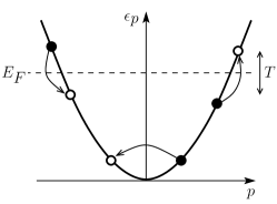
Figure 1: In the model of weakly interacting fermions the dominant backscattering process involves three particles: one near the bottom of the band and the other two near the left and right Fermi points Lunde et al. (2007).

The strong suppression of the backscattering rate means that at low temperatures the equilibration of the quantum liquid proceeds in two steps. First, the bosonic excitations come to thermal equilibrium with each other and their distribution function takes the form (4). This thermalization takes a relatively short time of order $\tau_{0}$. Second, over much longer time $\tau$ the backscattering processes equilibrate the zero mode $J$ with the bosons. During this time the velocity $u$ of the gas of bosonic excitations approaches the velocity $v_{d}$ of the liquid as the difference of the chemical potentials of the right and left movers $\Delta\mu$ relaxes to zero, see Eq. (6). The time dependences of $u$ and $\Delta\mu$ should follow the usual relaxation law

$$\frac{du}{dt}=-\frac{u-v_{d}}{\tau},\quad\frac{d}{dt}\Delta\mu=-\frac{\Delta\mu}{\tau}.$$ (7)

Expression (7) gives the formal definition of the equilibration time $\tau$.

In order to study the relaxation rate $\tau^{-1}$ at arbitrary interaction strength it is tempting to use the Luttinger liquid description of the system. However, this approach is incapable of describing the particles near the bottom of the band, Fig. 1, which are crucial for the equilibration of the system. More precisely, the bosonic Hamiltonian (1) provides an adequate description of the excitation spectrum of a quantum liquid only at low energies, namely $|\varepsilon|<D$, where the bandwidth $D\ll vp_{F}$. Indeed, for such excitations the spectrum can be linearized and consists of two independent branches, as required in the Luttinger model. On the other hand, any excitation with energy $|\varepsilon|\sim vp_{F}$ is not accounted for by the Hamiltonian (1).

This difficulty can be overcome as follows Matveev and Andreev (2012a). Because the small probability of an empty state near the bottom of the band plays the crucial role in the physics of equilibration, let us first consider the spectrum of the hole excitations. For non-interacting fermions a hole with momentum $Q$ can be defined as an excitation of the system obtained by moving a fermion from state $p_{F}-Q$ to $p_{F}$. For a system with concave spectrum, such as the one in Fig. 1, the hole represents the ground state of the system with the total momentum $Q$. We use this observation to generalize the concept of a hole excitation to the case of arbitrary interaction strength, and define the hole as the ground state of the system with momentum $Q$. Because moving a fermion from one Fermi point to the other changes momentum by $2p_{F}$ without changing the energy of the system, the energy $\varepsilon_{Q}$ of the hole is a periodic function of momentum and vanishes at $Q=0$, $\pm 2p_{F}$, $\pm 4p_{F}$, ….

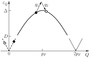
Figure 2: Spectrum of a hole excitation in a quantum liquid. The states with energies below $D$ are treated as excitations of the Luttinger liquid, whereas the higher-energy states are modeled as a mobile impurity. The hole can change its momentum by $\delta Q=q_{1}-q_{2}$ by absorbing a boson with momentum $q_{1}$ and emitting one with momentum $q_{2}$.

The holes with energies below the bandwidth $D$ have a nearly linear spectrum. They are accounted for in the Hamiltonian (1) as superpositions of various bosonic excitations with the same momentum. The holes with energies above $D$ are not included in the Hamiltonian (1) and are treated as mobile impurities in the Luttinger liquid Ogawa et al. (1992); Castro Neto and Fisher (1996); Pustilnik et al. (2006); Khodas et al. (2007); Pereira et al. (2009); Imambekov and Glazman (2009a, b); Gangardt and Kamenev (2010); Schecter et al. (2012). The exact value of the crossover energy scale $D$ is not important as long as it is small compared to the maximum energy of the hole $\varepsilon_{p_{F}}\sim vp_{F}$ and large compared to the temperature $T$.

The mechanism of equilibration can be described as follows. For simplicity, we assume from now on that the liquid is at rest, $v_{d}=0$. The gas of bosonic excitations equilibrates relatively quickly, and the occupation numbers of bosonic states take the form (4), which applies in the region $|q|<D/v$ represented by two straight dashed lines in Fig. 2. In a generic case the total momentum of the excitations in the initial state was not zero, so the Bose distribution (4) has a boost velocity $u\neq 0$. As a result of interactions between the bosons a small fraction of the particles are promoted above the energy $D$, where they are no longer described by the Hamiltonian (1). At arbitrary interaction strength the properties of these higher energy excitations are rather complicated, but the lowest energy excitation at a given momentum $Q$ is the hole. Since $\varepsilon_{Q}\gg T$, the occupation of the hole states is given by the Boltzmann factor

$$f(Q)=e^{-(\varepsilon_{Q}-uQ)/T}.$$ (8)

The presence of the correction $-uQ$ in the exponent is assured by the fact that the hole interacts and exchanges momentum with the thermalized bosons. As a result of many such collisions the hole, with small probability, may increase its momentum $Q$ above $p_{F}$, after which it is more likely to fall toward $Q=2p_{F}$ than return to the vicinity of $Q=0$, see Fig. 2. As the hole approaches $Q=2p_{F}$, it enters the region of linear spectrum at $\varepsilon_{Q}<D$, shown by dotted lines in Fig. 2. There it can again be viewed as a superposition of the bosonic excitations.

As a result of this rare sequence of scattering events the bosons have transferred to the hole the momentum $2p_{F}$. Due to the conservation of the total momentum (3), this decrease of momentum of the gas of excitations means that the zero mode $J=N^{R}-N^{L}$ has increased by 2, i.e., one fermion has been backscattered. Also, the decrease of the total momentum of the bosons means that the velocity $u$ has also decreased, in accordance with the relaxation law (7).

The equilibration proceeds very slowly because the hole must pass the point $Q=p_{F}$ in momentum space, where the occupation numbers are exponentially small. One therefore expects

$$\tau^{-1}=Ce^{-\Delta/T},\quad\Delta=\varepsilon_{p_{F}}.$$ (9)

To obtain the prefactor $C$, the kinetics of the scattering processes should be considered in more detail.

We start by noting that the equilibration rate is controlled by a small region of momentum space near $q=p_{F}$ where the energy of the hole is close to the maximum, $\Delta-\varepsilon_{Q}\lesssim T$. The width of this region can be estimated as $(m^{*}T)^{1/2}$, where we introduced the effective mass of the hole as

$$\frac{1}{m^{*}}=\left.-\frac{d^{2}\varepsilon_{Q}}{dQ^{2}}\right|_{Q=p_{F}}.$$ (10)

Although the region is narrow compared to $p_{F}$, it is wide compared to the typical change of the momentum of the hole in a single collision with bosonic excitations. Indeed, an elementary scattering event consists of the hole absorbing one boson and emitting another, see Fig. 2. Since the bosons are thermalized, the typical change of $Q$ is of order $T/v$, which is much smaller than $(m^{*}T)^{1/2}$ at $T\ll\Delta$. This estimate enables us to simplify the problem considerably.

The motion of the hole in momentum space is random and occurs in steps that are small compared to the size of the critical region near the barrier. Such diffusion in momentum space is described by the Fokker-Planck equation Lifshitz and Pitaevskii (1981) on the time-dependent distribution function $f(Q,t)$,

$$\partial_{t}f=-\partial_{Q}J,$$ (11)

where the probability current $J$ has the form

$$J=-\frac{B(Q)}{2}\left[\frac{\varepsilon_{Q}^{\prime}}{T}+\partial_{Q}\right]f.$$ (12)

Here prime denotes derivative with respect to $Q$, and $B(Q)$ has the meaning of the diffusion constant in momentum space. It is defined as

$$B(Q)=\sum_{\delta Q}[\delta Q]^{2}W_{Q,Q+\delta Q}$$ (13)

in terms of the rate $W_{Q,Q^{\prime}}$ of hole scattering from state $Q$ to $Q^{\prime}$.

In the steady state regime the Fokker-Planck equation (11) is solved by demanding that the probability current $J$ be independent of $Q$. To find the value of $J$ one has to impose the boundary conditions on the occupation numbers $f(Q)$ on the two sides of the barrier. Considering that the size of the crossover region in momentum space $(m^{*}T)^{1/2}$ is small compared with $p_{F}$, one can approximate Eq. (8) as

$$f(Q)=e^{-(\varepsilon_{Q}-up_{F})/T},\quad p_{F}-Q\gg(m^{*}T)^{1/2}.$$ (14)

This expression specifies the boundary condition upon $f(Q)$ to the left of the barrier. To find one to the right of the barrier we notice that the hole states with momenta $Q$ and $Q+2p_{F}$ are identical, and the occupation of states with $Q$ between $p_{F}$ and $2p_{F}$ is given by Eq. (8) with $Q\to Q-2p_{F}$. This yields

$$f(Q)=e^{-(\varepsilon_{Q}+up_{F})/T},\quad Q-p_{F}\gg(m^{*}T)^{1/2}.$$ (15)

Solving the first-order differential equation (12) with constant $J$ one finds that the boundary conditions (14) and (15) are satisfied for

$$J=u\,\frac{p_{F}B}{(2\pi m^{*}T^{3})^{1/2}}\,e^{-\Delta/T},$$ (16)

where we took the limit $u\to 0$ and denoted $B=B(2p_{F})$.

A non-vanishing constant $J$ means that $(L/h)J$ holes are passing any given point in momentum space in unit time. Each hole moving from the vicinity of $Q=0$ to that of $Q=2p_{F}$ takes momentum $2p_{F}$ out of the bosonic excitations. One therefore concludes that the total momentum of the bosons changes with time at the rate $\dot{P}_{b}=-2p_{F}(L/h)J$. Given that the momentum of the bosons distributed according to Eq. (4) is $P_{b}=(\pi LT^{2}/3\hbar v^{3})u$, we find $\dot{u}=-u/\tau$ with

$$\frac{1}{\tau}=\frac{3B}{\pi^{5/2}p_{F}^{2}}\left(\frac{vp_{F}}{T}\right)^{3}\left(\frac{p_{F}^{2}}{2m^{*}T}\right)^{1/2}e^{-\Delta/T}.$$ (17)

As expected, the equilibration rate has the exponential form (9). To fully evaluate the prefactor, however, one needs to study the hole scattering rate $W_{Q,Q^{\prime}}$ and obtain the diffusion constant (13).

IV Hole scattering rate

The scattering of a hole by bosonic excitations is a special case of the problem of dynamics of a mobile impurity in a Luttinger liquid Castro Neto and Fisher (1996). At low temperatures the leading scattering process involves two bosons moving in the opposite directions. By absorbing one boson and emitting the other the impurity can scatter from state $Q$ to a new state $Q^{\prime}$ without violating conservation of momentum and energy, Fig. 2. The authors of Ref. Castro Neto and Fisher, 1996 obtained the temperature dependence of the mobility of the impurity in a Luttinger liquid in this regime, $\mu\propto T^{-4}$. Using the expression $\mu=T/B$ for the mobility (see Lifshitz and Pitaevskii (1981), § 21) one concludes

$$B=\chi T^{5}.$$ (18)

The evaluation of the coefficient $\chi$ presents an interesting problem. Microscopic calculations can be performed in the special cases of either weak or strong interactions Micklitz et al. (2010); Matveev et al. (2010). Interestingly, one can also obtain a phenomenological expression for $\chi$ in terms of the spectrum of the mobile impurity (hole) in the Luttinger liquid Matveev and Andreev (2012a, b). Here we review the latter approach.

The diffusion constant $B$ in the expression (17) for the equilibration rate should be evaluated at $Q=p_{F}$. On the other hand, it is instructive to consider a more general problem and study the hole scattering rate $W_{Q,Q+\delta Q}$ in Eq. (13) for arbitrary $Q$. The latter can be found from the Fermi’s Golden rule

$$W_{Q,Q+\delta Q} = \frac{2\pi}{\hbar}\!\sum_{q_{1},q_{2}}\!|t_{q_{1},q_{2}}|^{2}N_{q_{1}}(N_{q_{2}}+1)\,\delta_{q_{1}-q_{2},\delta Q}$$ (19)

$$\times\delta(\varepsilon_{Q}-\varepsilon_{Q+\delta Q}+\hbar v|q_{1}|-\hbar v|q_{2}|),$$

where $t_{q_{1},q_{2}}$ is the matrix element of the process in which the hole absorbs the boson $q_{1}$ and emits the boson $q_{2}$, Fig. 2. Since the typical energies of the bosons are of order temperature, we will assume $|\delta Q|\ll p_{F}$. In this case one can easily obtain the momenta $q_{1}$ and $q_{2}$ from the conservation laws,

$$q_{1}=\frac{1}{2}\delta Q+\frac{v_{Q}}{2v}|\delta Q|,\quad q_{2}=-\frac{1}{2}\delta Q+\frac{v_{Q}}{2v}|\delta Q|.$$ (20)

Here $v_{Q}=\varepsilon_{Q}^{\prime}$ is the velocity of the hole with momentum $Q$. Using Eq. (20) one easily expresses the scattering rate as

$$W_{Q,Q+\delta Q}=\frac{L}{\hbar^{2}v}\,N_{q_{1}}(N_{q_{2}}+1)|t_{q_{1},q_{2}}|^{2}.$$ (21)

To evaluate the matrix element $t_{q_{1},q_{2}}$ we need to discuss the Hamiltonian of the Luttinger liquid in the presence of a mobile impurity.

We start by writing the Hamiltonian (1) in an alternative form Giamarchi (2004)

$$H_{0}=\frac{\hbar v}{2\pi}\int dx[K(\nabla\theta)^{2}+K^{-1}(\nabla\phi)^{2}],$$ (22)

where the two bosonic fields $\phi(x)$ and $\theta(x)$ satisfy the commutation relation

$$[\phi(x),\nabla\theta(x^{\prime})]=i\pi\delta(x-x^{\prime})$$ (23)

and the Luttinger liquid parameter $K$ depends on the interactions between particles. The case of non-interacting fermions corresponds to $K=1$.

The Hamiltonian (22) can be brought to the form (1) with the help of the following expressions for the fields $\phi$ and $\theta$ in terms of the bosonic operators:

$$\!\!\!\!\!\!\!\nabla\phi(x)\! \!=\! -i\sum_{q}\sqrt{\frac{\pi K|q|}{2\hbar L}}\,\mathrm{sgn}(q)(b_{q}+b_{-q}^{\dagger})e^{iqx/\hbar},$$ (24)

$$\!\!\!\!\!\!\!\nabla\theta(x)\! \!=\! i\sum_{q}\sqrt{\frac{\pi|q|}{2\hbar KL}}\,(b_{q}-b_{-q}^{\dagger})e^{iqx/\hbar}.$$ (25)

The advantage of the form (22) of the Hamiltonian is that the fields $\phi$ and $\theta$ have clear meanings in terms of the observables characterizing the quantum liquid. For instance, the field $\phi(x)$ accounts for the fluctuations of the density of the liquid

$$n(x)=n_{0}+\frac{1}{\pi}\nabla\phi(x),$$ (26)

where $n_{0}=N/L$ is the average density Giamarchi (2004). Similarly, the field $\theta$ is related to the momentum $\kappa$ of the liquid per particle

$$\kappa(x)=-\hbar\nabla\theta(x),$$ (27)

see, e.g., Ref. Matveev and Andreev, 2012b.

The coupling of the hole to bosonic excitations in the Luttinger liquid can now be obtained by considering the dependence $\varepsilon_{Q}(n,\kappa)$ of the energy of the hole on the density and momentum of the liquid. Using Eqs. (26) and (27) we expand $\varepsilon_{Q}(n,\kappa)$ in powers of the bosonic fields,

$$\varepsilon_{Q}(n,\kappa) = \varepsilon_{Q}(n_{0},0)+\frac{1}{\pi}\partial_{n}\varepsilon_{Q}\nabla\phi-\hbar\,\partial_{\kappa}\varepsilon_{Q}\nabla\theta$$ (28)

$$+\frac{1}{2\pi^{2}}\partial_{n}^{2}\varepsilon_{Q}(\nabla\phi)^{2}+\frac{\hbar^{2}}{2}\partial_{\kappa}^{2}\varepsilon_{Q}(\nabla\theta)^{2}$$

$$-\frac{\hbar}{\pi}\partial_{n}\partial_{\kappa}\varepsilon_{Q}\nabla\phi\nabla\theta+\ldots$$

Here all derivatives of $\varepsilon_{Q}(n,\kappa)$ are taken at $n=n_{0}$ and $\kappa=0$. Taking into account Eqs. (24) and (25) one sees that the second-order terms in Eq. (28) contain contributions in which a boson $q_{1}$ is absorbed and boson $q_{2}$ on the opposite branch is emitted. The respective matrix element has the form

$$t_{q_{1},q_{2}}^{(a)}=-\frac{\sqrt{|q_{1}q_{2}|}}{2\pi\hbar L}\,\partial^{2}_{LR}\varepsilon_{Q},$$ (29)

where we assumed that the hole is at $x=0$ and introduced the notation

$$\partial^{2}_{LR}=K\partial_{n}^{2}-\frac{(\pi\hbar)^{2}}{K}\partial_{\kappa}^{2}.$$ (30)

In addition to the terms coupling the hole to two bosons, Eq. (28) contains the contribution linear in bosonic operators:

$$i\partial_{L}\varepsilon_{Q}\sum_{q<0}\sqrt{\frac{|q|}{2\pi\hbar L}}\,(b_{q}-b_{q}^{\dagger})-i\partial_{R}\varepsilon_{Q}\sum_{q>0}\sqrt{\frac{|q|}{2\pi\hbar L}}\,(b_{q}-b_{q}^{\dagger}),$$ (31)

where

$$\partial_{L}=\sqrt{K}\partial_{n}-\frac{\pi\hbar}{\sqrt{K}}\partial_{\kappa},\quad\partial_{R}=\sqrt{K}\partial_{n}+\frac{\pi\hbar}{\sqrt{K}}\partial_{\kappa}.$$ (32)

The linear coupling terms (31) also contribute to the matrix element $t_{q_{1},q_{2}}$, but in the second order perturbation theory,

$$t_{q_{1},q_{2}}^{(b)} = -\frac{\sqrt{|q_{1}q_{2}|}}{2\pi\hbar L}\left[\frac{\partial_{L}\varepsilon_{Q+q_{1}}\partial_{R}\varepsilon_{Q}}{\varepsilon_{Q}+vq_{1}-\varepsilon_{Q+q_{1}}}\right.$$ (33)

$$\hskip 50.00008pt\left.+\frac{\partial_{R}\varepsilon_{Q-q_{2}}\partial_{L}\varepsilon_{Q}}{\varepsilon_{Q}-\varepsilon_{Q-q_{2}}-v|q_{2}|}\right],$$

where we assumed $q_{1}>0$ and $q_{2}<0$, i.e., positive $\delta Q$ as in Fig. 2. It is important to account for the corrections to the momentum of the hole in the numerator which are due to the fact that the two perturbations of the form (31) act on the states of the hole with different values of $Q$.

The expression (33) can be simplified by taking advantage of the smallness of $q_{1}\sim q_{2}\sim\delta Q\ll p_{F}$. The expression in the brackets appears to scale as $1/\delta Q$. This term is obtained by neglecting corrections to $Q$ in the numerator and linearizing the denominators in $q_{1}$ and $q_{2}$. However, for the specific values (20) of the boson momenta the two contributions in the brackets cancel each other. Evaluating the next order terms in $q_{1}$ and $q_{2}$ one finds

$$\!\!\!\!\!\!\!\!\!t_{q_{1},q_{2}}^{(b)} \!=\! -\frac{\sqrt{|q_{1}q_{2}|}}{2\pi\hbar L}\Bigg{[}\frac{1}{m_{Q}^{*}}\frac{\partial_{L}\varepsilon_{Q}}{v+v_{Q}}\frac{\partial_{R}\varepsilon_{Q}}{v-v_{Q}}$$ (34)

$$\hskip 40.00006pt+\partial_{L}v_{Q}\frac{\partial_{R}\varepsilon_{Q}}{v-v_{Q}}-\partial_{R}v_{Q}\frac{\partial_{L}\varepsilon_{Q}}{v+v_{Q}}\Bigg{]}.$$

Here the momentum dependent effective mass of the hole is defined by $1/m_{Q}^{*}=-\varepsilon_{Q}^{\prime\prime}$. The first term in Eq. (34) originates from the expansion of the denominators of Eq. (33) to second order in $q_{1}$ and $q_{2}$, whereas the remaining two terms are obtained by accounting for linear corrections in the numerators.

Finally, one more contribution to the scattering matrix element $t_{q_{1},q_{2}}$ is obtained when the hole couples to a single boson, Eq. (31), which in turn splits into two. The latter matrix element involves three bosons and should therefore originate from cubic in $\phi$ and $\theta$ corrections in the Hamiltonian. For a fluid at rest the symmetry allows only for even powers of $\theta$, so the correction must have the form

$$H_{\alpha}=\int dx\big{[}\alpha_{\theta}(\nabla\phi)(\nabla\theta)^{2}+\alpha_{\phi}(\nabla\phi)^{3}\big{]}.$$ (35)

The values of the coefficients $\alpha_{\theta}$ and $\alpha_{\phi}$ can be related to the density dependences of the parameters $v$ and $K$ of the quadratic Hamiltonian (22) by considering the correction to the total Hamiltonian $H_{0}+H_{\alpha}$ caused by a small change of particle density $\delta n$. As a result one obtains Matveev and Andreev (2012b)

$$\alpha_{\theta}=\frac{\hbar}{2\pi^{2}}\,\partial_{n}(vK),\quad\alpha_{\phi}=\frac{\hbar}{6\pi^{2}}\,\partial_{n}\left(\frac{v}{K}\right).$$ (36)

In order to find a contribution to $t_{q_{1},q_{2}}$ we need the matrix element of $H_{\alpha}$ that absorbs a boson with momentum $q_{1}$ on one branch and emits a boson $q_{2}$ on the other branch. Using Eq. (36) we obtain

$$\frac{i\mathrm{sgn}(q_{1})}{\sqrt{2\pi\hbar L}}\frac{v\partial_{n}K}{\sqrt{K}}\sqrt{|q_{1}q_{2}(q_{1}-q_{2})|}\,b_{q_{2}}^{\dagger}b_{q_{1}}\big{(}b_{q_{2}-q_{1}}+b_{q_{1}-q_{2}}^{\dagger}\big{)}.$$ (37)

The second order calculation of the matrix element $t_{q_{1},q_{2}}$ with perturbations (37) and (31) yields

$$t_{q_{1},q_{2}}^{(c)}=-\frac{\sqrt{|q_{1}q_{2}|}}{2\pi\hbar L}\frac{v\partial_{n}K}{\sqrt{K}}\bigg{(}\frac{\partial_{R}\varepsilon_{Q}}{v-v_{Q}}+\frac{\partial_{L}\varepsilon_{Q}}{v+v_{Q}}\bigg{)}.$$ (38)

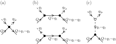
Figure 3: The three types of processes contributing to the scattering matrix element $t_{q_{1},q_{2}}$. (a) The first order process, in which the hole couples to two bosons. (b) The second order processes involving two perturbations, each coupling the hole to one of the two bosons. (c) The second order process where the hole couples to a virtual boson, which is separately coupled to bosons $q_{1}$ and $q_{2}$.

The three types of processes leading to hole scattering with absorption of boson $q_{1}$ and emission of boson $q_{2}$ are illustrated in Fig. 3. Their total is given by

$$t_{q_{1},q_{2}}=-\frac{\sqrt{|q_{1}q_{2}|}}{2\pi\hbar L}\,Y_{Q},$$ (39)

where

$$Y_{Q}=\partial^{2}_{LR}\varepsilon_{Q}+\frac{1}{m_{Q}^{*}}\frac{\partial_{L}\varepsilon_{Q}}{v+v_{Q}}\frac{\partial_{R}\varepsilon_{Q}}{v-v_{Q}}+\partial_{L}v_{Q}\frac{\partial_{R}\varepsilon_{Q}}{v-v_{Q}}$$ (40)

$$\hskip 5.0pt-\partial_{R}v_{Q}\frac{\partial_{L}\varepsilon_{Q}}{v+v_{Q}}+\frac{v\partial_{n}K}{\sqrt{K}}\bigg{(}\frac{\partial_{R}\varepsilon_{Q}}{v-v_{Q}}+\frac{\partial_{L}\varepsilon_{Q}}{v+v_{Q}}\bigg{)}.$$

An alternative way of evaluating the scattering matrix element involves performing a unitary transformation that eliminates the linear coupling (31) of the hole to the bosons Matveev and Andreev (2012b). Upon this transformation only the quadratic coupling remains, which is then evaluated in the first order, similarly to Eq. (29). The resulting expression given by Eqs. (49) and (50) of Ref. Matveev and Andreev, 2012b is equivalent to Eq. (39).

Using the expression (39) for the scattering matrix element in combination with Eqs. (21) and (13) one easily recovers the temperature dependence (18). The coefficient $\chi$ takes the form

$$\chi=\frac{4\pi Y_{p_{F}}^{2}}{15\hbar^{5}v^{6}}.$$ (41)

Equations (17), (18), and (41) provide a complete expression for the equilibration rate of a one-dimensional quantum liquid in terms of the spectrum of hole excitations and its dependences on the particle density $n$ and the momentum per particle $\kappa$.

V Discussion

In this paper we discussed the equilibration of a one-dimensional quantum liquid of interacting fermions. The conventional Luttinger liquid theory Haldane (1981); Giamarchi (2004) of these systems neglects the processes of backscattering. In many cases this is an excellent approximation since the corresponding scattering rates are exponentially small at low temperatures, Eq. (17). However, the Luttinger liquid approximation does not enable one to treat a number of interesting phenomena in which the backscattering plays the crucial role.

One example is the conductance of a long uniform quantum wire. The Luttinger liquid theory predicts perfect conductance quantization in these devices, regardless of the interaction strength Maslov and Stone (1995); Ponomarenko (1995); Safi and Schulz (1995). On the other hand, it is easy to show that at weak electron-electron interactions a correction to conductance appears due to the backscattering processes Lunde et al. (2007); Micklitz et al. (2010). Interestingly, an expression for the conductance of a quantum wire can be obtained for any interaction strength Matveev and Andreev (2011),

$$G=\frac{e^{2}}{h}\left(1-\frac{\pi^{2}}{3}\,\frac{T^{2}}{v^{2}p_{F}^{2}}\frac{L}{L+2v\tau}\right).$$ (42)

The backscattering gives rise to a negative correction to the quantized conductance, which grows with temperature and with the length of the wire $L$. In short wires the correction $\delta G\propto\tau^{-1}$ is exponentially small, but it saturates at $\delta G\sim-(e^{2}/h)(T/vp_{F})^{2}$ in long wires.

Temperature dependent corrections to conductance of quantum wire devices have been observed in multiple experiments Thomas et al. (1996); Kristensen et al. (2000); Cronenwett et al. (2002). The data shows excellent quantization of conductance at lowest temperatures and a negative correction developing as the temperature is raised. These observations are in qualitative agreement with Eq. (42). In comparing the data with theory it is important to keep in mind that our discussion so far has ignored spins, which appear to play an important role in experiments. The result (42) can be generalized to include spins Matveev and Andreev (2011), but the evaluation of the equilibration rate of a system with spins is still an open problem. Another complication is that most experiments study rather short wires which may not be treated as uniform.

Our discussion of the equilibration rate did not assume Galilean invariance of the system. On the other hand, momentum conservation was assumed. Thus the results do not automatically apply to systems of interacting particles in periodic potentials, such as spin chains. In such systems umklapp scattering by the external potential may facilitate equilibration. On the other hand, electrons in GaAs quantum wires have an essentially quadratic spectrum $\epsilon_{p}=p^{2}/2m$, where $m$ is the effective mass of electron in this material. Such electron system is Galilean invariant, which leads to a few simplifications. First, the Luttinger liquid parameter in this case is determined by velocity of the bosons, $K=\pi\hbar n/mv$. Second, the dependence of the excitation energy on momentum $\kappa$ has the simple form Lifshitz and Pitaevskii (1980)

$$\varepsilon_{Q}(n,\kappa)=\varepsilon_{Q}(n)+Q\frac{\kappa}{m}.$$ (43)

For momenta $Q$ in the vicinity of $p_{F}$ one can expand $\varepsilon_{Q}(n)=\Delta(n)-(Q-p_{F})^{2}/2m^{*}$ and find

$$Y_{p_{F}}=K\left(\Delta^{\prime\prime}+\frac{\Delta^{\prime 2}}{m^{*}v^{2}}-\frac{2v^{\prime}}{v}\Delta^{\prime}\right).$$ (44)

Upon substitution into Eq. (41) one recovers the results of Ref. Matveev and Andreev, 2012a for equilibration rate in Galilean invariant systems obtained by a different technique. It is worth noting that in this case the equilibration rate is fully determined by the density dependences of the velocity of bosonic excitations $v$ and the maximum energy of the hole $\Delta$.

Although our main focus was on interacting systems of fermions, the approach and the results should be equally applicable to systems of bosons. Similar techniques have been recently applied to dynamics of dark solitons and mobile impurities in bosonic fluids Gangardt and Kamenev (2010); Schecter et al. (2012). Finally, it is worth mentioning that in integrable models apart from energy and momentum there are multiple additional conserved quantities, and one expects that no equilibration of the system should take place. In particular one should find $\tau^{-1}=0$. This conjecture has been checked Matveev and Andreev (2012a) for the Calogero-Sutherland Sutherland (2004) and Lieb-Liniger Lieb and Liniger (1963) models. More generally, one expects Matveev and Andreev (2012b) that for integrable models the quantity $Y_{Q}$ given by Eq. (40) should vanish for any $Q$.