Melting of graphene clusters

Abstract

Density-functional tight-binding and classical molecular dynamics simulations are used to investigate the structural deformations and melting of planar carbon nano-clusters $C_{N}$ with N=2-55. The minimum energy configurations for different clusters are used as starting configuration for the study of the temperature effects on the bond breaking/rotation in carbon lines (N$<$6), carbon rings (5$<$N$<$19) and graphene nano-flakes. The larger the rings (graphene nano-flake) the higher the transition temperature (melting point) with ring-to-line (perfect-to-defective) transition structures. The melting point was obtained by using the bond energy, the Lindemann criteria, and the specific heat. We found that hydrogen-passivated graphene nano-flakes (C_NH_M) have a larger melting temperature with a much smaller dependence on its size. The edges in the graphene nano-flakes exhibit several different meta-stable configurations (isomers) during heating before melting occurs.

I Introduction

The study of the melting of crystals is one of the important subjects in the field of phase transitions. Melting phenomena occurs at the surface of bulk materials Dash and needs a microscopic theory for a deep understanding. Nano-scale molecular clusters due to their size-dependent properties show melting processes different from those of bulk materials and infinite size two-dimensional materials. The melting of nano-clusters has received considerable attention recently and it was found that nano-clusters melt typically below their corresponding bulk melting temperature Koga ; Ercolessi ; Lewis . This is due to the higher chemical reactivity of nano-clusters which is the consequence of the increased accessible surface and the presence of more free dangling bonds.

The microscopic behavior of nano-clusters at finite temperature can be understood theoretically using a variety of molecular dynamics (MD) methods Cleveland ; Rytkonen ; Joshi ; Chuang ; Beck ; Bas and can be determined directly by experiment Schmidt ; Shvartsburg ; Breaux . In most of the simulations the microscopic structure is characterized in terms of bond-lengths and their average fluctuations over many cycles of the MD simulation Rey ; Rodeja ; Li .

Since the discovery of two dimensional materials, i.e. graphene Castro ; Geim and hexagonal boron nitride sheet zettle2009 the melting of these new materials have attracted many researches Zakhar . The new 2D crystalline materials respond to an increasing temperature by loosing their lattice symmetry, e.g. Zakharchenko et al. Zakhar studied the high temperature behavior of graphene using atomistic simulations. The melting temperature of graphene was estimated to be about 4900 K. Before melting first Stone-Wales defects appear because of their smallest energy barrier. When increasing temperature further eventually spaghetti-type of carbon chains are formed that spread in 3D. A similar melting process can be found for carbon nanotubes using a much smaller critical Lindemann parameterKaiwang . The melting temperature of perfect single-wall carbon nanotubes (SWNTs) was estimated to be around 4800 K Kaiwang . In graphene nano-ribbons different types of edges (i.e. zig-zag, armchair) affect the melting process differently, e.g. Lee et al. Lee found that at 2800 K edge reconstruction occurs in a zig-zag ribbon.

In our previous work we found that the minimum energy configuration for flat carbon clusters up to N=5 atoms consists of a line of carbons kosi1 (linear chain) which is in agreement with ab-initio raghavachari calculations. Carbon planar rings were found for 5$<$N$<$19 and graphene nano-flakes are minimum energy configurations for larger N kosi . Here we investigate the effect of temperature on those minimum energy configurations and find the melting temperature of such small flat carbon clusters, as function of the size of the clusters.

A systematic study of the size dependence of the melting temperature is still lacking as well as the effect of H-passivation of the edge atoms on the melting process. We will present such a study and identify the different fundamental steps in the melting process. We found that graphene nano-flakes have a lower transition temperature as compared to bulk graphene and graphene nanoribbons. We also found that H-passivated clusters exhibit higher melting temperature than non H-passivated clusters. In all cases, once clusters are defected they can be in different meta-stable structures (none-planar isomers). We will compare our results with those found for graphene and graphene nano-ribbons. The Lindemann index increases with respect to temperature in all cases while its slope versus temperature increases (decreases) linearly for the ring structures (graphene nano-flakes). Furthermore, using ab-initio molecular dynamics simulation we analyse the energy change due to defect formation.

This paper is organized as follows. In Sec. II, we introduce the atomistic model and the simulation method. Sec. III contains our main results and a discussion of the melting of graphene-like clusters and H-passivated clusters. Sec. IV gives information on the topology of the defects. The effect of defects on the total energy is introduced in Sec. V. In Sec. VI, we conclude the paper.

II Simulation Method and Model

II.1 Minimum energy configurations

The second-generation of Brenner reactive empirical bond order (REBO) potentialbren2 function between carbon atoms is used in the present work. All the parameters for the Brenner potential can be found in Ref.bren2 and are therefore not listed here.

In Fig. 1 we depict the minimum energy configurations for carbon clusters which are carbon lines up to 5 atoms (Fig. 1(a)), carbon rings for up to 18 atoms (Fig. 1(b)), graphene nano-flakes up to 55 atoms (Fig. 1(c)) and hydrogen passivated graphene nano-flakes (Fig. 1(d)). These configurations were obtained using conjugate gradient minimization method in our previous works kosi ; kosi1 . The carbon line structures are energetically favorable structures among other possible geometries (isomers) which are shown in Fig. 1 of Ref. kosi1 , i.e. two for $C_{3}$, 6 for $C_{4}$ and 11 for $C_{5}$. Among all possible carbon nano-clusters (isomers) for 5$<$N$<$19 atoms the ground state are a single ring, see Fig. 1(b). Increasing the number of carbon atoms, graphene nano-flakes are formed which can have pentagon and heptagon defects in addition to common hexagons, see Fig. 1(c). Notice that by passivating the dangling bonds by hydrogens in graphene flakes some structural deformations are possible. In Fig. 1(d) the minimum energy configurations for hydrogen passivated graphene nano-flakes (which were obtained by passivating the structures in Fig. 1(c)) are shown. It is interesting to note that most of these minimum configuration structures have zig-zag edges which is due to the higher stability of these kind of edges as compared to arm-chair edges Seifert .

In the present work we study the temperature effects on the structural transition and melting properties of these minimum energy configurations. Using molecular dynamic simulations, we obtain the new configuration of the above mentioned clusters at a given temperature T. This temperature is maintained during the whole simulation by the Langevin thermostat rui . The MD time step was taken to be 0.5 fs. Different properties of the cluster were measured during the MD simulation of $10^{6}$ MD steps (500 ps) at fixed temperature.

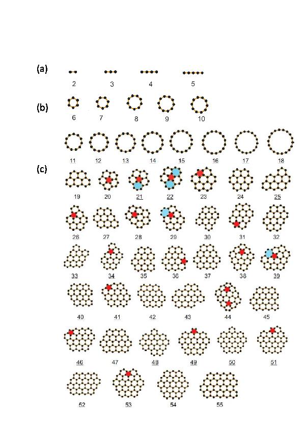
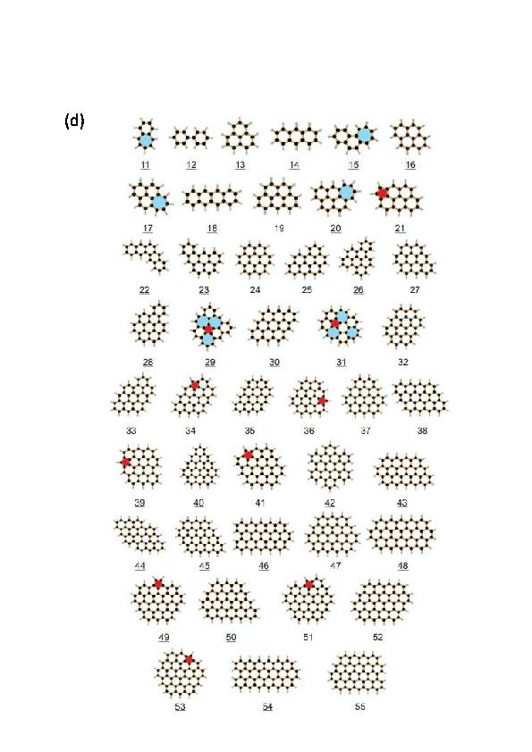
Figure 1: (Color online) The investigated configurations for carbon lines (a) carbon rings (b) and graphene nano-flakes (c). Pentagons (heptagons) are colored red (blue). By H-passivating the structures in (c) most of them transit to new structures (shown in (d)) which are indicated by underlined numbers.

II.2 Density-functional tight-binding molecular dynamics

In order to have an independent test of the results obtained from the bond order potential for the melting of graphene nano-flakes, we also performed independent calculations using the DFTB/MD (density-functional based tight-binding molecular dynamics) approach which is a QM/MD technique based on a tight binding method using an approximate density-functional formalism Porezag ; Elstner ; Frauenheim . DFTB passed several benchmark tests with first principle density functional theory (DFT) Porezag ; Zheng ; Alberto for carbon structures. Alberto et al. Alberto showed that DFTB accurately reproduced the structures and energies for a range of point defects such as vacancies and Stone-Wales defects in graphene. Migration barriers for vacancies and Stone-Wales defect formation barriers are also accurately reproduced. Kuc et al Seifert studied the stability of graphene nano-flakes using DFTB and by comparing their results with DFT, good agreement was found between the two methods. Although this method is two orders of magnitude faster than DFT but for the purpose of this work where we will study about 90 different configurations it will be computationally expensive. Therefore, we will use DFTB for a few N-values in order to show the accuracy of our classical MD simulation by considering one of the line carbons, two of the rings, five of graphene nano-flakes and six of H-passivated systems.

II.3 Lindemann criterion and specific heat

The root-mean-square relative bond length variance (Lindemann criterion) in addition to the caloric curve gives a reasonable computational method for determining the melting point of nano-clusters. It is sensitive to any change in the bond lengths at the microscopic scale. The Lindemann criterion March ; Ziman is often used in molecular dynamics and Monte Carlo simulations in order to estimate the melting temperature in three dimensional bulk systems Blome ; Shen , two dimensional materials Zakhar and nano-clusters erik . We used the distance-fluctuation of the Lindemann index ($\delta$) in order to identify the melting temperature of our nano-clusters. For a system of N atoms, the local Lindemann index for the ${\imath}^{th}$ atom in the system is defined as Zhou ; Ding

$$\delta_{i}=\frac{1}{N-1}\sum_{j(\neq i)}\frac{\sqrt{\langle r_{ij}^{2}\rangle_{T}-\langle r_{ij}\rangle_{T}^{2}}}{\langle r_{ij}\rangle_{T}}$$ (1)

and the system-average Lindemann index is then given by

$$\delta=\frac{1}{N}\sum_{i}\delta_{i}$$ (2)

where $r_{ij}$ is the distance between the ${\imath}^{th}$ and ${\jmath}^{th}$ atoms, N is the number of atoms and $\langle\cdot\cdot\cdot\rangle_{T}$ denotes the thermal average at temperature T. The Lindemann index  Lindemann depends on the specific system and its size which varies in the range 0.03-0.15, e.g.  it was recently Zhou applied to nanoparticles and homopolymers and found to be in the range of 0.03-0.05, for Ni nanoclusters it was found to be around 0.08 erik and for carbon nanotubes about 0.03 Kaiwang .

For sufficiently low temperature there is no structural transition and the atoms exhibit thermal fluctuation around the $T=0$ equilibrium position. The oscillation amplitude increases linearly with temperature due to Hooke’s regime for the atomic vibrations leading to a linear increase of the Lindemann index with T. At higher temperature, the anharmonic vibrations (non-linear effects) become important and the Lindemann index exhibits a nonlinear dependence on T. The particle oscillation amplitude increases faster than linear with T, but the system does not melt yet, since the arrangement of atoms have still some ordered structure, i.e. solid-liquid coexistence state. For small nano-clusters the latter is related to not well defined small three dimensional structures. In general, melting occurs when the Lindemann index increases very sharply with T over a small T-range. In this study we will assume that the melting point is around the sharp jump in $\delta$, i.e. when the system becomes almost a random coil. We will show that the Lindemann index adequately indicates the structural deformation (melting-like transition) of carbon nano-clusters. The obtained linear regime in $\delta$ is smoother than some of the previous studies erik for small nano-clusters. Therefore, we will not only use the critical value of $\delta$ to determine the melting point but we will also pay particular attention to the temperature dependence of the Lindemann index when identifying the melting temperature.

In addition to the Lindmann index, the total energy (caloric curve) and specific heat variation versus T are two common quantities which can be used to determine the phase transition. We calculated the specific heat $C_{P}$ using the equationHsu

$$C_{P}(T)=\frac{\langle E^{2}_{total}\rangle_{T}-\langle E_{total}\rangle_{T}^{2}}{k_{B}T^{2}},$$ (3)

where $E_{total}=\sum_{i}\frac{1}{2}m_{i}v_{i}^{2}+E_{P}$. The average potential energy of the system was calculated as a function of temperature. In the crystalline state the total energy of the system increases almost linearly with temperature, and then after the critical temperature is reached, it increases more steeply which is a signature of melting. We will show that for graphene nano-flake with 54 carbon atoms (C₅₄ and C₅₄H₂₀) energy and heat capacity calculations are found to be consistent with the results for the melting temperature that we obtained from the analysis of the Lindemann index.

III Results and Discussion

III.1 Energy

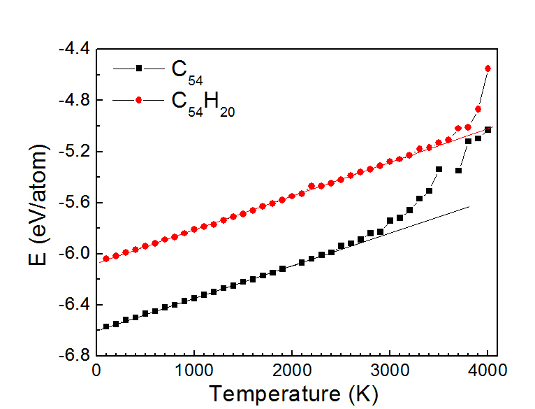
Figure 2: (Color online) The temperature dependence of the total energy of the graphene nanoflake C₅₄ and the H-passivated C₅₄H₂₀ using the REBO potential.

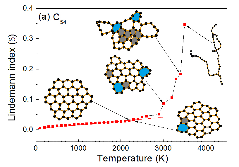
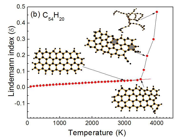
Figure 3: (Color online) The temperature dependence of the Lindemann index for the cluster (a) without H-passivated C₅₄ and (b) with H-passivated C₅₄H₂₀. The insets show typical C (a) and C-H (b) atoms configurations where the solid areas indicate topological defects.

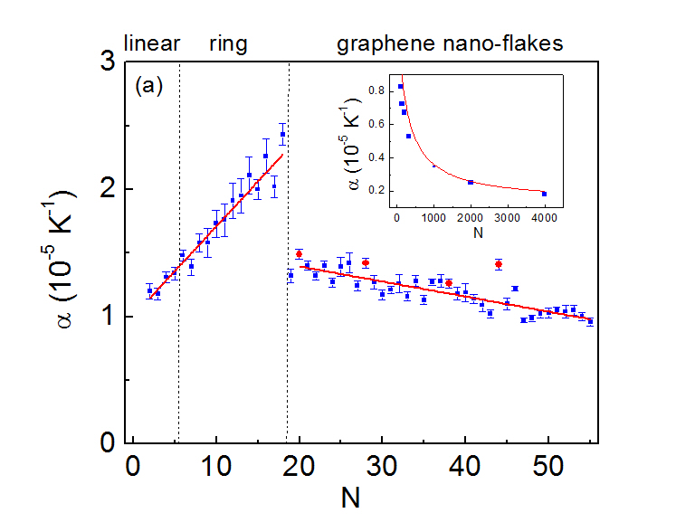
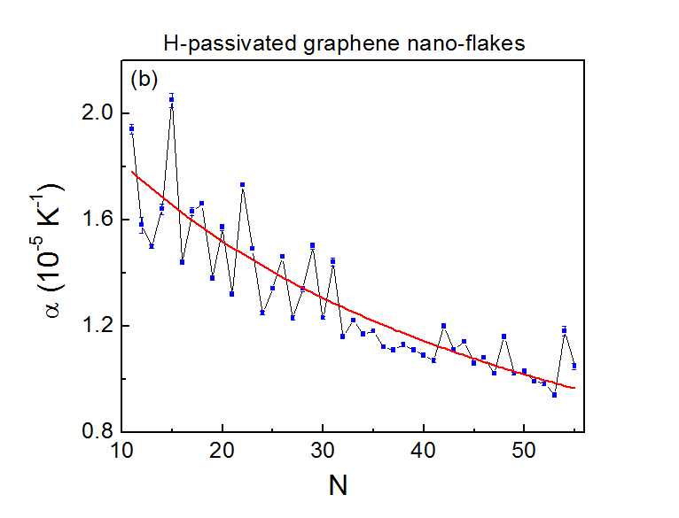
Figure 4: (Color online) The low temperature rate of the Lindmann index versus the number of atoms in (a) graphene nano-flakes and (b) H-passivated graphene nano-flakes. The red solid lines are linear fits to the average behavior of $\alpha$. The bowl-like clusters are shown by red solid circles (a). In the inset, the same quantity versus the number of atoms in graphene nano-flakes for N up to 4000 (a).

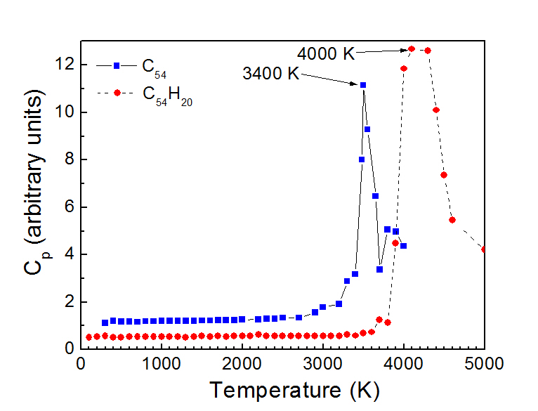
Figure 5: (Color online) The temperature dependence of the specific heat for C₅₄ and C₅₄H₂₀.

The temperature dependence of the total energy of graphene nano-flakes (C₅₄ and C₅₄H₂₀) are depicted in Fig. 2 using the Brenner potential. For C₅₄ the energy increases linearly at low temperatures and starts to deviate from the linear behavior around T=2300 K due to the reconstruction of the zigzag edges and the formation of pentagon-heptagon (5-7) defects. It indicates that the first nucleation of melting starts around 2300 K and modifies the edges. As temperature increases, the formation of pentagon, heptagon, 5-7 defects or 5-8-5 are possible and eventually large ring structures results in a dramatic increase of the energy. Above T= 3400 K, there is a sharp increase in the energy showing a completely molten structure.

For C₅₄H₂₀, passivation removes the dangling orbitals of the C atoms at the edge, lowering the reactivity, and increasing the stability of the cluster. It was found that unlike previous case (without H-passivated clusters), the H-passivated clusters keep their initial atomic arrangement up to higher temperature and therefore no noticeable change in the geometry was found for temperatures up to T=3200 $K$ for C₅₄H₂₀. The binding energy of the H-passivated clusters are larger than for non-passivated clusters. As temperature increases further to T=3500 K, some hydrogen atoms start to dissociate and finally the clusters convert into hydrocarbon chains around T=4000 K showing larger melting temperature than the corresponding non-passivated cluster which has a melting temperature of 3400 K (see Fig. 2).

III.2 Lindemann index

Fig. 3 displays the variation of the Lindemann index with temperature for (a) C₅₄ and (b) C₅₄H₂₀. The corresponding structures during heating for a few typical temperatures are shown in the insets. The slope of the function $\delta(T)$ (i.e. $\alpha=\frac{d\delta}{dT}$) is plotted in Fig. 4 for all studied structures of Fig. 1. The value of $\alpha$ (before reaching the melting point) increases monotonically for the carbon lines (Fig. 1(a)) and carbon rings (Fig. 1(b)). This is an indication of keeping the initial configuration while non-linear effects indicate defect formation, e.g. 5-7 defects in C₅₄. The increase of $\alpha$ is fitted in Fig. 4 by the red line for $N\leq 18$ which is given by the function $\alpha(N)=a+b\times N$, where: a=1.005 ($\pm 0.032)\times 10^{-5}K^{-1}$ and b=0.070 ($\pm 0.004)\times 10^{-5}K^{-1}$. Note that increasing temperature forces the system to be out-of-planed, e.g. the rings at finite temperature are not circles and become deformed ellipsoids in 3D.

For N $\geq$ 19, there is a sudden decrease in $\alpha$ of size $\Delta\alpha=1.11\times 10^{-5}K^{-1}$ due to the strong $sp^{2}$ bonds within the graphene like clusters (instead of simple covalent bonds in the carbon lines and rings) and a decreasing number of dangling bonds. The average behavior is fitted by the red line $\alpha(N)=a+b\times N$, where: a= 1.63($\pm 0.06)\times 10^{-5}K^{-1}$ and b=-0.012 ($\pm 0.001)\times 10^{-5}K^{-1}$. For bowl like clusters (N=20, 28, 38, 44), due to the presence of topological defective pentagon inside the cluster, the $\alpha$ value is larger as compared to their neighbor clusters. Therefore the important message is that dangling bonds and any kind of defects enhance anharmonic effects.

In order to investigate the effect of large size samples we also calculated $\alpha$ for a few large graphene nano-flakes and found that $\alpha$ decreases with N (see inset in Fig. 4). The maximum considered size of graphene nano-flakes had 4000 atoms. For large N, one expects saturation of $\alpha$, thus a line with negative slope which we fitted for 19 $\leq$ N $\leq$ 55 should not be applicable. Therefore, we used the fit $\alpha(N)=\alpha(\infty)+a/(1+b\times N)$, where: $\alpha(\infty)=0.134\times 10^{-5}K^{-1}$, a=1.213 ($\pm 0.005)\times 10^{-5}K^{-1}$ and b=48.7 ($\pm 4.9)\times 10^{-4}$ on large clusters. These results clearly indicate that $\delta$ for small graphene nano-flakes is considerably larger than for larger flakes and graphene. Although the Lindemann index was defined initially in the thermodynamical limit (bulk material) we show that it is also a good parameter to investigate the effect of temperature and melting of nano size systems.

For completeness, we calculated $\alpha$ for H-passivated graphene nano-flakes for 11$\leq$ N $\leq$ 55 number of C-atoms and found that $\alpha$, on average, decreases with N (see Fig. 4(b)). The average behavior is fitted by the red line $\alpha(N)=a/(1+b\times N)$, where: a=2.262 ($\pm 0.115)\times 10^{-5}K^{-1}$ and b=0.024 ($\pm 0.003)\times 10^{-5}$. The rapid decrease in the latter fit (Fig. 4(b)) is an indication of the role of H-passivation in making the graphene nano-flakes more stable against temperature for larger N.

III.3 Specific heat

The calculated specific heat curve for C₅₄ is shown in Fig 5. A clear peak is observed in the specific heat with a maximum around 3400 K which we identify as the melting temperature, and which is close to the results from the analysis using the Lindemann index. The specific heat curve is also shown for C₅₄H₂₀ (see red symbols in Fig. 5) and displays a peak around T=4000 K which is identified as the melting temperature, showing good agreement with the result of the previous caloric curve (see Fig. 2). A discontinuity or a sharp peak  in the heat capacity is a clear indication of a phase transition. However, here this is not exactly a solid-to-liquid like transition, but rather a nano-flake to random-coil transition.

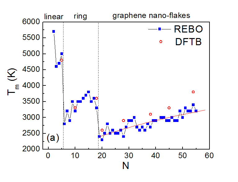
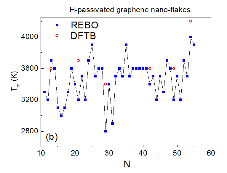
Figure 6: (Color online) The melting temperature versus the number of atoms using Brenner (square symbols) and DFTB (open circles) for (a) nano-graphene and (b) hydrogenated nano-graphene. The error bar is 50 K.

Table 1: Melting temperature for large clusters

$N$	$T_{m}(K)$
98	3800
142	4000
194	4100
322	4200
1000	4400
graphene	5500

III.4 Melting-temperature

The melting temperature for all studied clusters $C_{N}(2\leq N\leq 55)$ is shown in Fig. 6(a). The different parts separated by vertical dashed lines correspond to the three set of systems shown in Figs. 1(a-c). For small linear structures except for the carbon dimer the melting temperature increases with the number of atoms (linear chains have bond breaking).

In order to check if for large N we approach the melting temperature of bulk graphene, we also calculated the melting temperature of three large graphene nano-flakes and graphene (by performing a simulation having 4000 atoms with periodic boundary condition with NPT ensemble) and presented the results in Table I. From Table I it is clear that large flakes approach slowly the melting temperature of graphene, i.e. 5500  K. As a comparison the melting temperature reported in Ref. Zakhar by using the LCBOPII potential was 4900 K and in Ref. Brad using REBO was 5200 K.

We fitted the melting temperature for graphene like clusters (red curve in Fig. 6(a)) by the function $T_{m}(N)=T_{m}^{bulk}-(a/(b+N))$ where $a=417(\pm 47)\times 10^{3}K$, $b=119.34(\pm 17.71)$ and $T_{m}^{bulk}=5500K$ for graphene was taken from our simulation. We included the results of Table I in this fit. We also calculated the melting temperature using DFTB for the clusters with N=5, 10, 18, 20, 28, 38, 45, and 54 (C₅₄) which are represented by the open red circles in Fig. 6(a). They are found to slightly overestimate the melting temperature but exhibit clearly the same N-dependent trend.

For completeness, we also calculated the melting temperature of H-passivated clusters for N=11-55 C-atoms (Fig. 6(b)). The melting temperature fluctuates around T=3500 K (note that on average T_m increases slowly with N with large fluctuations imposed on it) for most of the clusters with minima for N=29 and N=31 C-atoms due to the large number of defects in their structures. The clusters which have pentagon defects on the boundary usually have lower melting temperature then the others. Here, the melting temperature for the clusters N=13, 21, 29, 42, 49 and 54 were also calculated using DFTB (open red circles in Fig. 6(b)). In most cases the DFTB results are close to the Brenner potential results indicating that the Brenner bond order potential is a useful specialized potential for thermal effects in hydrocarbons.

IV Topology of Defects

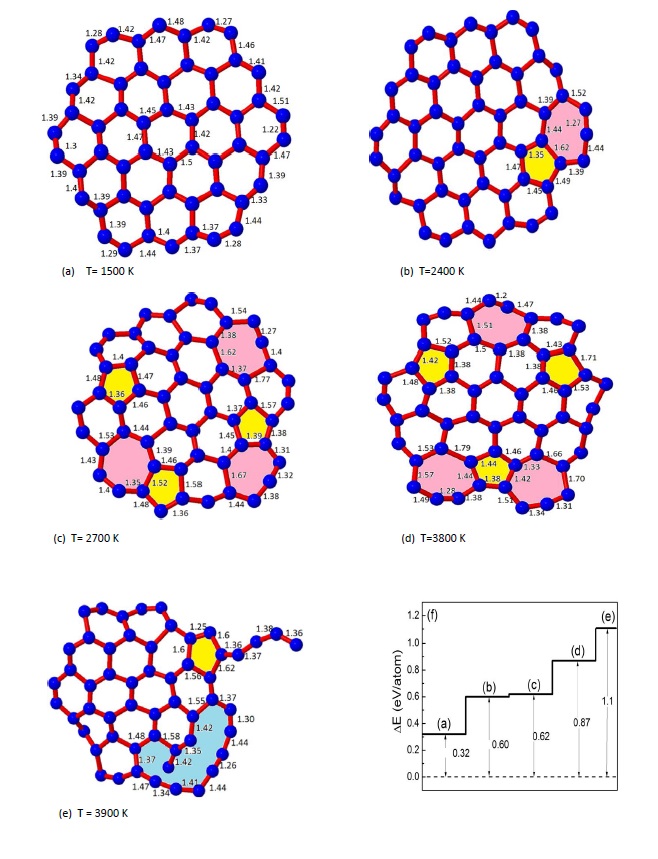
Figure 7: (Color online) Five different snap shots of the cluster C₅₄ at different temperature (a-e). Bond lengths are indicated in the figure and the colored areas indicate defect structures. (f) The corresponding energy diagram for the five snap shots.

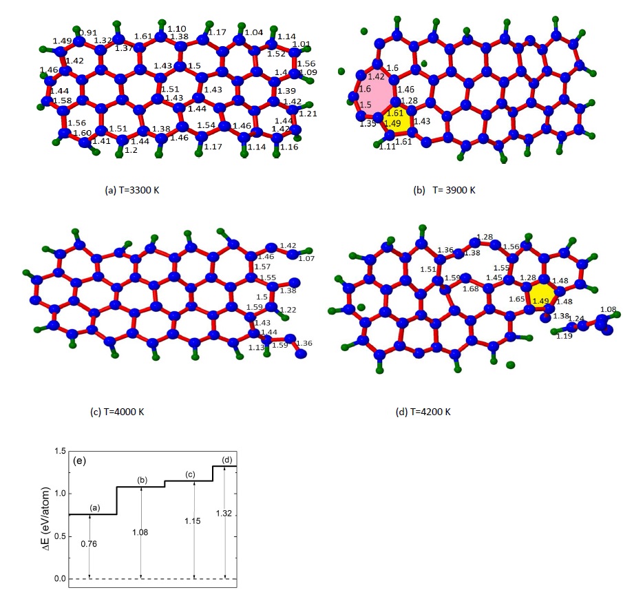
Figure 8: (Color online) Four different snap shots of the cluster C₅₄H₂₀ at different temperature (a-d). Bond lengths are indicated in the figure and the colored areas indicate defect structures. (e) The corresponding energy diagram for the four snap shots.

In this section we consider the topology of some of the defects which are created during the melting process of C₅₄ using DFTB calculations. We found that these defects have a pronounced effect on the melting behavior of the system whose mechanism is different from both graphene and graphene nanoribbons. At low temperature the probability of defect creation is small and the flakes remains perfect which for this low temperature range is similar to graphene Zakhar and graphene nanoribbon Koskinen . Increasing temperature (above about 2300 K) the energy increases and the system can overpass certain potential barriers and we found that during the molecular dynamics simulation the system transits from one metastable state to another, see Figs. 7(a-b). We show five snap shots of C₅₄ at different temperature in Fig. 7. The transition temperature at which the edge reconstruction occurs, i.e. T$\sim$ 2400 K is lower than those found for defect formation in graphene, i.e. 3800 K and edge reconstruction in graphene nano-ribbons Lee , i.e. 2800 K. As seen in Fig. 7(b) the first defected structure has one heptagon and one pentagon at the edge with different bond lengths. The energy difference between non-defected (Fig. 7(a)) and defected (Fig. 7(b)) one is about 0.28  eV/atom which is due to the 900  K difference in the temperature between these two structures. In Fig. 7 the next defected configuration due to a 1200 K increase in temperature is shown which has more heptagon and pentagon defects (colored parts). By increasing temperature further we found some transition in the defected parts and even an edge reconstruction from heptagon to hexagon and vise versa until the appearance of a tail-like part in the cluster, Fig. 7(e). The melting temperature for C₅₄ as shown in Fig. 6(a) (open circle symbol) is around 3900 K. This melting temperature is lower than those found for graphene. The larger the graphene nano-flake the higher the melting temperature. For small graphene nano-flakes the larger number of dangling bonds results in a lower melting temperature and larger boundary effects. The energy diagram for five snap shots is depicted in Fig. 7(f). The presented energy is the difference between the total energy of the system at given temperature and the zero temperature total energy for C₅₄.

In Figs. 8(a-d) we show the temperature effect on C₅₄H₂₀. In Fig. 8(e) the corresponding energy diagram is shown. Hydrogens become released at T=3900 K. Notice that DFTB calculations for the shown configurations in Figs. 8(a-d) were performed separately, i.e. we do not increase temperature of sample Fig. 8(a) in order to obtain Fig. 8(b), but instead we performed four different calculations for these four snap shots. Thus we do not expect that we have sequential configurations.

V Conclusion

Using molecular dynamics simulation and the Lindemann index for melting supplemented with results for the total energy and the specific heat, we investigated the melting of carbon nano clusters. The melting temperature of small carbon flakes is lower than those for graphene and graphene nano-ribbons. The Lindemann index is sensitive to temperature and is a good quantity for determining when structural deformations of the clusters start to occur. The melting temperature of small flakes on average increases versus the number of atoms in carbon nano clusters. All clusters investigated show premelting behavior with different premelting intervals. For certain N-values defects are already present inside the cluster which lowers the melting temperature. H-passivated clusters have a higher melting temperature than the non H-passivated clusters with the same number of C-atoms. The melting temperature for H-passivated clusters is larger than for non-passivated clusters. Our simulation results also help to understand the formation of defects (due to the increase of temperature) in the graphene nano-flake which can then be applied to understand the growth and thermal treatment of nanographene. We supplemented our analysis by DFTB calculations which confirm the N-dependence of the melting temperature.

VI ACKNOWLEDGMENTS

This work was supported by the EU-Marie Curie IIF postdoc Fellowship/299855 (for M.N.-A.), the ESF-EuroGRAPHENE project CONGRAN, the Flemish Science Foundation (FWO-Vl), and the Methusalem Foundation of the Flemish Government.

References

- (1) J. G. Dash, Rev. Mod. Phys. 71, 1737 (1999).
- (2) K. Koga, T. Ikeshoji, and K. I. Sugawara, Phys. Rev. Lett. 92, 115507 (2004).
- (3) F. Ercolessi, W. Andreoni, and E. Tosatti, Phys. Rev. Lett. 66, 911 (1991).
- (4) L. J. Lewis, P. Jensen and J. L. Barrat, Phys. Rev. B 56, 2248 (1997).
- (5) C. L. Cleveland, W. D. Luedtke, and U. Landman, Phys. Rev. B 60, 5065 (1999).
- (6) A. Rytkönen, H. Häkkinen, and M. Manninen, Phys. Rev. Lett. 80, 3940 (1998).
- (7) K. Joshi, D. G. Kanhere, and S. A. Blundell, Phys. Rev. B 66, 155329 (2002).
- (8) F. C. Chuang, C. Z. Wang, S. Ögüt, J. R. Chelikowsky, and K. M. Ho, Phys. Rev. B 69, 165408 (2004).
- (9) T. L. Beck and R. S. Berry, J. Chem. Phys. 88, 3910 (1988).
- (10) B. S. Bas, M. J. Ford, and M. B. Cortie, J. Phys.: Condens. Matter 18, 55 (2006).
- (11) M. Schmidt, R. Kusche, W. Kronmüller, B. von Issendorff and H. Haberland, Phys. Rev. Lett. 79, 99 (1997).
- (12) A. A. Shvartsburg and M. F. Jarrold, Phys. Rev. Lett. 85, 2530 (2000).
- (13) G. A. Breaux, R. C. Benirschke, T. Sugai, B. S. Kinnear, and M. F. Jarrold, Phys. Rev. Lett. 91, 215508 (2003).
- (14) C. Rey, L. J. Gallego, J. García-Rodeja, J. A. Alonso, and M. P. Iñiguez, Phys. Rev. B 48, 8253 (1993).
- (15) J. García-Rodeja, C. Rey, L. J. Gallego and J. A. Alonso, Phys. Rev. B 49, 8495 (1994).
- (16) T. X. Li, Y. L. Ji, S. W. Yu and G. H. Wang, Solid State Commun. 116, 547 (2000).
- (17) A. H. Castro Neto, F. Guinea, N. M. R. Peres, K. S. Novoselov, and A. K. Geim, Rev. Mod. Phys. 81, 109 (2009).
- (18) A. K. Geim and K. S. Novoselov, Nat. Mater. 6, 183 (2007).
- (19) N. Alem, R. Erni, C. Kisielowski, M. D. Rossell, W. Gannett, and A. Zettl, Phys. Rev. B 80, 155425 (2009).
- (20) K. V. Zakharchenko, A. Fasolino, J. H. Los, and M. I. Katsnelson, J. Phys.: Condens. Matter 23, 202202 (2011).
- (21) K. Zhang, G. M. Stocks, and J. Zhong, Nanotechnology 18, 285703 (2007).
- (22) G. D. Lee, C. Z. Wang, E. Yoon, N. M. Hwang, and K. M. Ho, Phys. Rev. B 81, 195419 (2010).
- (23) D. P. Kosimov, A. A. Dzhurakhalov, and F. M. Peeters, Phys. Rev. B 78, 235433 (2008).
- (24) K. Raghavachari and J. S. Binkley, J. Chem. Phys. 87, 2191 (1987).
- (25) D. P. Kosimov, A. A. Dzhurakhalov, and F. M. Peeters, Phys. Rev. B 81, 195414 (2010).
- (26) D. W. Brenner, O. A. Shenderova, J. A. Harrison, S. J. Stuart, B. Ni, and S. B. Sinnott, J. Phys.: Condens. Matter 14, 783 (2002).
- (27) A. Kuc, T. Heine, and G. Seifert, Phys. Rev. B 81, 085430 (2010).
- (28) L. Rui, H. Yuan-Zhong, W. Hui, and Z. Yu-Jun, Chin. Phys. 17, 4253 (2008).
- (29) D. Porezag, T. Frauenheim, T. Kohler, G. Seifert, and R. Kaschner, Phys. Rev. B 51, 12947 (1995).
- (30) M. Elstner, D. Porezag, G. Jungnickel, J. Elsner, M. Haugk, T. Frauenheim, S. Suhai, G. Seifert, Phys. Rev. B 58, 7260 (1998).
- (31) T. Frauenheim, G. Seifert, M. Elstner, T. Niehaus, C. Kohler, M. Sternberg, Z. Hajnal, A. Di Carlo, S. Suhai, J. Phy.: Condens. Matter 14, 3015 (2002).
- (32) G. Zheng, S. Irle, K. Morokuma, Chem. Phys. Lett. 412, 210 (2005).
- (33) A. Zobelli, V. Ivanovskaya, P. Wagner, I. Suarez-Martinez, A. Yaya, and C. P. Ewels, Phys. Status Solidi B 249, 276 (2012).
- (34) N. H. March and M. P. Tosi, Introduction to Liquid State Physics (World Scientific, Singapore, 2002).
- (35) J. M. Ziman, Principles of the Theory of Solids (Cambridge University, Cambridge 1972).
- (36) K. Sokolowski-Tinten, C. Blome, J. Blums, A. Cavalleri, C. Dietrich, A. Tarasevitch, I. Uschmann, E. Förster, M. Kammler, M. Horn-von-Hoegen, and D. von der Linde, Nature (London) 422, 287 (2003).
- (37) G. Shen, V. B. Prakapenka, M. L. Rivers, and S. R. Sutton, Phys. Rev. Lett. 92, 185701 (2004).
- (38) E. C. Neyts and A. Bogaerts, J. Phys. Chem. C 113, 2771 (2009).
- (39) Y. Zhou, M. Karplus, K. D. Ball, and R. S. Berry, J. Chem. Phys. 116, 2323 (2002).
- (40) F. Ding, K. Bolton, and A. Rosen, Eur. Phys. J. D 34, 275 (2005).
- (41) F. A. Lindemann, Physik. Z. 11, 609 (1910). H. Lowen, Phys. Rep. 237, 249 (1994). J. H. Bilgram, Phys. Rep. 153, 1 (1987).
- (42) P. J. Hsu, J. S. Luo, S. K. Lai, J. F. Wax, and J. -L. Bretonnet, J. Chem. Phys. 129, 194302 (2008).
- (43) M. Neek-Amal and F. M. Peeters, Phys. Rev. B 83, 235437 (2011).
- (44) B. Steele, R. Perriot, V. Zhakhovsky, and I. Oleynik, http://meetings.aps.org/link/BAPS.2012.MAR.W12.3.
- (45) P. Koskinen, S. Malola, and H. Häkkinen, Phys. Rev. Lett. 101, 115502 (2008).