A New Bayesian Test to test for the Intractability-Countering Hypothesis

Abstract

We present a new test of hypothesis in which we seek the probability of the null conditioned on the data, where the null is a simplification undertaken to counter the intractability of the more complex model, that the simpler null model is nested within. With the more complex model rendered intractable, the null model uses a simplifying assumption that capacitates the learning of an unknown parameter vector given the data. Bayes factors are shown to be known only up to a ratio of unknown data-dependent constants–a problem that cannot be cured using prescriptions similar to those suggested to solve the problem caused to Bayes factor computation, by non-informative priors. Thus, a new test is needed in which we can circumvent Bayes factor computation. In this test, we undertake generation of data from the model in which the null hypothesis is true and can achieve support in the measured data for the null by comparing the marginalised posterior of the model parameter given the measured data, to that given such generated data. However, such a ratio of marginalised posteriors can confound interpretation of comparison of support in one measured data for a null, with that in another data set for a different null. Given an application in which such comparison is undertaken, we alternatively define support in a measured data set for a null by identifying the model parameters that are less consistent with the measured data than is minimally possible given the generated data, and realising that the higher the number of such parameter values, less is the support in the measured data for the null. Then, the probability of the null conditional on the data is given within an MCMC-based scheme, by marginalising the posterior given the measured data, over parameter values that are as, or more consistent with the measured data, than with the generated data. In the aforementioned application, we test the hypothesis that a galactic state space bears an isotropic geometry, where the (missing) data comprising measurements of some components of the state space vector of a sample of observed galactic particles, is implemented to Bayesianly learn the gravitational mass density of all matter in the galaxy. In lieu of an assumption about the state space being isotropic, the likelihood of the sought gravitational mass density given the data, is intractable. For a real example galaxy, we find unequal values of the probability of the null–that the host state space is isotropic–given two different data sets, implying that in this galaxy, the system state space constitutes at least two disjoint sub-volumes that the two data sets respectively live in. Implementation on simulated galactic data is also undertaken, as is an empirical illustration on the well-known O-ring data, to test for the form of the thermal variation of the failure probability of the O-rings.

journalname math.PR/0000000

t1Lecturer of Statistics at Department of Mathematics, University of Leicester and Associate at Department of Statistics, University of Warwick

1 Introduction

Model selection is a very common exercise faced by practitioners of different disciplines, and substantial literature exists in this field (Kass and Raftery, 1995; Berger and Pericchi, 2001; Chipman et al., 2001; Ghosh and Samanta, 2001; Barbieri and Berger, 2004; O’Hagan, 1995; Casella et al., 2009). In this context, some advantages of Bayesian approaches, over frequentist methods have been reported (Berger and Pericchi, 2004; Robert, 2001). Much has been discussed in the literature to deal with the computational challenge of Bayes factors (Han and Carlin, 2000; Chib and Jeliazkov, 2001; Casella et al., 2009, to name a few). At the same time, methods have been advanced as possible resolutions when faced with the challenge of improper priors on the system variables (Aitkin, 1991; Berger and Pericchi, 1996a; O’Hagan, 1995). Nonetheless, Bayes factor computation persists as a challenge, especially in the context of non-parametric and multimodal inference on a high-dimensional state space (Link and Barker, 2006).

In this paper we discuss a new test of hypothesis that is aimed at finding support in the available data for the null that the state space that the observed variable lives in, is endowed with a simple symmetry, namely isotropy. In an isotropic state space, the density at a given point depends only on the magnitude of the state space vector to that point, and not on the inclination of this vector to a chosen direction. This assumption about the geometry of the state space is invoked to allow us to refer to an application, in which the sought model parameter vector can be estimated from the data, only under the simplistic assumption that the state space is isotropic. In lieu of such an assumption, the likelihood of the unknown parameters given the data is rendered intractable. Upon the estimation of the sought parameters, given the data at hand, we want to review how bad this assumption of isotropy of the state space is, in the considered data.

The application we elude to above, involves the estimation of the density of all gravitating matter in a real galaxy NGC 3379 for which multiple data sets are measured for two distinct types of galactic particles (Douglas et al., 2007; Bergond et al., 2006). The sought model behaviour function is the gravitational mass density function of all matter–dark as well as luminous–in this real galaxy. One of the burning questions in science today is the understanding of dark matter. The quantification of the distribution of dark matter in our Universe, at different length scales, is of major interest in Cosmology (Roberts and Whitehurst, 1975; Sofue and Rubin, 2001; Salucci and Burkert, 2000; de Blok et al., 2003; Hayashi et al., 2007). At scales of individual galaxies, the relevant version of this exercise is the estimation of the density of the gravitational mass of luminous as well as dark matter content of these systems. Readily available data on galactic images, can in principle be astronomically modelled to quantify the gravitational mass density of the luminous matter in the galaxy, (Gallazzi and Bell, 2009; Bell and de Jong, 2001); such luminous matter is however, only a minor fraction of the total that is responsible for the gravitational field of the galaxy since the major fraction of the galactic gravitational mass is contributed to by dark matter (Kalinova, 2014). Astronomical measurements that bear signature of the gravitational effect of all (dark+luminous) matter in a galaxy are hard to achieve in “early-type” galaxies, the observed images of which is typically elliptical in shape. Of some such astronomical measurements, noisy and partially missing information on velocities of individual galactic particles have been implemented to learn the density of all gravitating matter in the galaxy (Côté et al., 2001; Genzel et al., 2003; Chakrabarty and Raychaudhury, 2008).

In this application, the null states that the native space of the data variable is isotropic. This null is nested within a more complex model in which, the data lives in a state space that is not necessarily isotropic. However, in this application, estimation of the model parameters is not possible under this more complex model, given the data; in fact, even the formulation of the likelihood of the unknown parameters given the data, is not possible unless the null is invoked. When we refer below to the complex model being “intractable”, we imply the impossibility of both formulating and computing the likelihood under this model. Given this nature of the complex model, we find that the posterior odds of the null model given two independent data sets is known only upto a ratio of unknown constants, where these constants are the uncomputable probabilities of the considered data sets. In form, the indeterminacy of the posterior odds appears similar to that of the Bayes Factor when non-informative priors are used on the model parameters–in that case, the priors are known only upto an unknown constant, so that the the Bayes Factor is left indeterminate upto a ratio of these unknown constants. However, unlike the indeterminacy caused by non-informative priors, the indeterminacy of the posterior odds in the considered application is entirely data dependent, motivating us to seek a new test that bypasses computation of Bayes Factors. This test helps find support in a data set for a null, or can find the ratio of supports for two nulls given two different data sets. When the application is in the latter context, the test permits usage of data sets of widely different sizes, and the dimensionality of the model parameter vectors sought under the different models could also be very different from each other. Lastly, very little prior information may be available on the model parameter vectors in one or both models.

This new test involves generating data from the model in which the null is true. Though in principle, it is possible to compare the marginalised posterior of the model parameter given measured data to that given generated data, a ratio of these posteriors may confound the comparison of supports in two differently sized data sets for respective nulls, with model parameters of different dimensionalities. Such describes the galactic application discussed above. In such applications, support in a data for a null is given by the probability of the null conditional on the data, which in turn is the posterior of the model parameter marginalised over those parameter values that are more or equally consistent with the measured data, than is minimally achieved given the data that is generated when the null is true.

The paper is organised as follows. Section 2 discusses the general background to the estimation of the unknown model parameter vector and its specific formulation in the context of the application undertaken in this work. Section 3.1 clarifies the formulation of the null as the assertion that the state space that the data variable lives in, is isotropic. In this same section we discuss the vagaries of an intractable alternative that the null is nested within and motivate the need for a new test, which is introduced in Section 4. Differences between this new test and FBST are discussed in Section 4.1. An empirical illustration of this test on the well-known O-ring data is presented in Section 4.2. The implementation of this new test in the context of our galactic application is discussed in Section 5. Such implementation is illustrated on simulated and real data. The work with the simulated data is presented in Section 6 while the application to the data of a real galaxy is included in Section 7. The paper is concluded with a discourse on the implications of the results, in Section 8.

2 Case Study

In the application that we are interested in, the state space vector $\boldsymbol{W}\in{\cal W}\subseteq{\mathbb{R}}^{6},\boldsymbol{W}=(X_{1},X_{2},X_{3},V_{1},V_{2},V_{3})^{T}$, where $\boldsymbol{X}=(X_{1},X_{2},X_{3})^{T}$ and $\boldsymbol{V}=(V_{1},V_{2},V_{3})^{T}$. In the application, $\boldsymbol{X}$ is the three-dimensional location and $\boldsymbol{V}$ the velocity vector of a particle in the system. The measurables include some components of $\boldsymbol{X}$ and some components of $\boldsymbol{V}$–the measurable vector is $\boldsymbol{U}=(X_{1},X_{2},V_{3})^{T}$ so that the data set is ${\bf D}=\{\boldsymbol{u}_{k}\}_{k=1}^{N_{data}}$. Thus, $\boldsymbol{U}\in{\cal U}\subset{\cal W}$. We are interested in estimating the model parameter vector $\boldsymbol{\theta}\in{\cal S}$. In the application, $\boldsymbol{\theta}=(\Psi_{1},\ldots,\Psi_{N_{eng}},\rho_{1},\rho_{2},\ldots,\rho_{N_{x}})^{T}$, where $\boldsymbol{\rho}=(\rho_{1},\rho_{2},\ldots,\rho_{N_{x}})^{T}$ and $\boldsymbol{\Psi}=(\Psi_{1},\Psi_{2},\ldots,\Psi_{N_{eng}})^{T}$ which respectively, are the discretised versions of an unknown model function $\rho(\boldsymbol{X})$ and the state space $pdf$. In our application, $\rho(\boldsymbol{X})$ is the density of gravitational mass of all (dark+luminous) matter in the galaxy, in which $\boldsymbol{U}$ has been observed for a sample of $N_{data}$ galactic particles.

The reason for reducing our ambition from learning the full functions $\rho(\boldsymbol{X})$ and the state space $pdf$, to their discretised forms–namely $\boldsymbol{\rho}$ and $\boldsymbol{\Psi}$ respectively–is the lack of “training data”, which in this context, is the data set comprising a set of values of the data variable $\boldsymbol{U}$, generated at chosen values of $\rho(\boldsymbol{X})$ and the state space $pdf$. However, we do not know the physics underlying the relation between the unknown functions and $\boldsymbol{U}$–such is the system at hand. This results in the inability to generate the value of $\boldsymbol{U}$ at a chosen value of $\rho(\boldsymbol{X})$ and the state space $pdf$, i.e. results in the unavailability of training data. In this situation, we cannot take the usual approach of statistical learning using training data, to train a model of the relationship between the measurable and unknown functions, to thereafter predict the unknown function by implementing the available measurements (test data) in this model (Neal, 1998).

Consequently, we are left with the possibility of discretising the support of the unknown functions and estimate the values of the functions in each resulting grid cell, treating these values as independent of each other without invoking a correlation structure. Thus we can only learn the discretised forms of these unknown functions, i.e. learn the vector $\boldsymbol{\rho}$ where the $i$-th component of $\boldsymbol{\rho}$ is the value of $\rho(\boldsymbol{X})$ in the $i$-th grid cell that the support of $\rho(\boldsymbol{X})$ is discretised into (and likewise for the vector $\boldsymbol{\Psi}$, a component of which is the value of the state space $pdf$ over a grid-cell, where the support of this $pdf$ is discretised into grid-cells).

Details of the estimation of $\boldsymbol{\rho}$ and $\boldsymbol{\Psi}$ from ${\bf D}$ is discussed in Section S-1 of the Supplementary Material. It is to be noted that this estimation is markedly non-trivial given that the measurements are of parameters $X_{1},X_{2},V_{3}$ while the sought unknown function $\rho(\boldsymbol{X})$ is defined over $\boldsymbol{X}=(X_{1},X_{2},X_{3})^{T}$ and the sought unknown state space density is defined over the state space vector $\boldsymbol{W}=(X_{1},X_{2},X_{3},V_{1},V_{2},V_{3})^{T}$. Thus the measurables live only in a sub-volume inside the state space, i.e. ${\cal U}\subset{\cal W}$. In other words, the measurables are sampled from the density $\nu(\boldsymbol{U})$ of the $\boldsymbol{U}$ vector, where $\nu(\boldsymbol{U})$ is achieved by marginalising the state space density over the non-measurables, i.e. over $X_{3},V_{1},V_{2}$. The likelihood function is written in terms of $\nu(\boldsymbol{U})$ convolved with the density of the errors in the measurables. Importantly, this likelihood is intractable unless the state space ${\cal W}$ admits isotropy. So we assume an isotropic state space and achieve the likelihood of the unknowns $\boldsymbol{\rho}$, $\boldsymbol{\Psi}$ given ${\bf D}$. Relevant priors are invoked and we write the posterior of the unknowns given the data; posterior inference is carried out using Metropolis-Hastings.

For NGC 3379, data include missing data on the three observable state space coordinates of 164 galactic particles called planetary nebulae (PNe)–that are the end states of certain massive stars–as reported by Douglas et al. (2007). In addition, there is data on 29 of another type of galactic particles called globular clusters (GCs) that are clusters of stars–reported by Bergond et al. (2006).

NGC 3379, or M 105, seems to have initiated its journey within the observational domain, in neglect - though Pierre Mechain is credited with its discovery in 1781, it did not initially make it to Messier’s catalogue. Amends were made later in 1947, when it was among four new objects that were “added to the accepted list of Messier’s catalogue as nos. 104, 105, 106 and 107” (from Helen Sawyer, 1947). In spite of this early inattention, NGC 3379 has been studied carefully in the past few years. Romanowsky et al. (2003) advanced the idea that NGC 3379 is one of the five “naked galaxies”, that were tracked using the data on the observed PNe samples in these five galaxies . Such claims were contested by Dekel et al. (2005), though Douglas et al. (2007) defend the earlier result of Romanowsky et al. (2003) by analysing the PNe data in NGC 3379. For this galaxy, Douglas et al. (2007) also report one value of gravitational mass at a chosen distance from the galactic centre, obtained from using the GCs data in this galaxy (Bergond et al., 2006). This single value obtained using the GC data, is shown to concur with the estimate based on PNe data, within error bars. Weijmans and et al. (2009) cannot infer the distribution of the total gravitational mass distribution in this galaxy since the halo contribution is an unknown model parameter for them. Coccato et al. (2009) and Pierce and et al. (2006) report the characterisation of this galaxy using PNe and GC data respectively.

It is to be noted that by “training data” in the first part of this section, we imply data that consists of pairs of design points and measurable values generated at this design point, while in the context of Bayes Factor literature, “training samples” or “training data” typically imply data that mimic the available set of measurements and can therefore be “real” (i.e. are samples of the available measurements), or “imaginary” i.e. sampled from the posterior predictive under the null, given the available measurements.

3 Testing for the assumption of an isotropic state space given the data at hand

3.1 The null hypothesis

If the state space ${\cal W}$ is isotropic, the state space density is an isotropic function of $\boldsymbol{X}$ and $\boldsymbol{V}$, where the state space vector is $\boldsymbol{W}=(X_{1},X_{2},X_{3},V_{1},V_{2},V_{3})^{T}$.

Remark 3.1.

If a real-valued function $g(\cdot,\cdot)$ of two vectors ${\bf a},{\bf b}\in{\mathbb{R}}^{m}$, is an isotropic function of ${\bf a},{\bf b}$, then $g({\bf a,b})=g({\bf Q}{\bf a},{\bf Q}{\bf b})$, for any orthogonal transformation matrix ${\bf Q}\in{\mathbb{R}}^{(m\times m)}$ (Truesdell et al., 2004; Wang, 1969). We recall from the theory of scalar valued functions of two vectors, that if $g(\cdot,\cdot)$ is an isotropic function, its set of invariants with respect to ${\bf Q}$ is ${\Upsilon}_{Q}=\{{\bf a}\cdot{\bf a},{\bf b}\cdot{\bf b},{\bf a}\cdot{\bf b}\}$ where “$\cdot$” is the inner product of 2 vectors. Then, the isotropic function of two vectors, $g({\bf a},{\bf b})$, admits the representation $g({\Upsilon}_{Q})\equiv g({\bf a}\cdot{\bf a},{\bf b}\cdot{\bf b},{\bf a}\cdot{\bf b})$ (Truesdell et al., 2004; Liu, 2002).

In our application, $\boldsymbol{X}\cdot\boldsymbol{V}$=0 identically so that it follows from Remark 3.1 that if the state space density $f(\boldsymbol{X},\boldsymbol{V})$ is an isotropic function of $\boldsymbol{X}$ and $\boldsymbol{V}$, then it will depend on $\boldsymbol{X}$ and $\boldsymbol{V}$ via the form $f(\boldsymbol{X}\cdot\boldsymbol{X},\boldsymbol{V}\cdot\boldsymbol{V})$, i.e. $f(X^{2},V^{2})$, since $\boldsymbol{X}\cdot\boldsymbol{X}=\parallel\boldsymbol{X}\parallel^{2}=X^{2}=(X_{1}^{2}+X_{2}^{2}+X_{3}^{2})$, where $\parallel\cdot\parallel$ is the $L^{2}$-norm of a vector. Similarly, $\boldsymbol{V}\cdot\boldsymbol{V}=\parallel\boldsymbol{V}\parallel^{2}=V^{2}=(V_{1}^{2}+V_{2}^{2}+V_{3}^{2})$. Thus, in this application, any function$f(X^{2},V^{2})$ is an isotropic scalar-valued function of $\boldsymbol{X}$ and $\boldsymbol{V}$. To summarise, any function that depends on $\boldsymbol{X}$ and $\boldsymbol{V}$ via the $L^{2}$-norms of the $\boldsymbol{X}$ and $\boldsymbol{V}$ vectors, is an isotropic function of the 2 vectors $\boldsymbol{X}$ and $\boldsymbol{V}$.

In our application, it then follows that if we define a simple function of $X$ ($:=\sqrt{X^{2}}={\parallel\boldsymbol{X}\parallel}$) and $V$ ($:={\parallel\boldsymbol{V}\parallel}$) as: $E(X,V):=\Phi(X)+\eta(V)$, the state space density that bears the form $\Psi(E)$ is an isotropic function of $\boldsymbol{X}$ and $\boldsymbol{V}$, implying that state space ${\cal W}$ is isotropic. Here $\Psi(\cdot)\geq 0$ is any function; (the constraint of non-negativity stems from non-negativity of the state space density). Thus, the null that the $i$-th data set at hand (${\bf D}_{i}$) is sampled from an isotropic state space density function $f_{i}(\boldsymbol{X},\boldsymbol{V})$, is expressed as:

$$H_{0}^{(i)}:f_{i}(\boldsymbol{X},\boldsymbol{V})=\Psi_{i}(E(X,V)),\quad{\mbox{where}}\quad\Psi_{i}(\cdot)\geq 0,$$ (3.1)

where in our application, $i=1,2$. That the null model is different in the 2 cases suggests that while data ${\bf D}_{1}$ lives in the isotropic state space ${\cal W}_{1}$ under the null $H_{0}^{(1)}$, the data ${\bf D}_{2}$ does not necessarily live in the same state space but rather in a different state space ${\cal W}_{2}$ in general, which is isotropic under the null $H_{0}^{(2)}$.

We have discussed in Section 2 that lack of training data causes replacement of the learning of the unknown gravitational mass density function $\rho(\boldsymbol{X})$ by its discretised version, namely the vector $\boldsymbol{\rho}=(\rho_{1},\ldots,\rho_{N_{x}})^{T}$. Similarly, the state space density function $f(\boldsymbol{X},\boldsymbol{V})=\Psi(E(X,V))$ under the assumption of isotropy, cannot be learnt, but in its place, its discretised version is learnt, namely the vector $\boldsymbol{\Psi}=(\Psi_{1},\ldots,\Psi_{N_{E}})^{T}$. Then the sought model parameter vector, learnt using data ${\bf D}_{i}$ is $\boldsymbol{\theta}_{i}=(\Psi_{1}^{(i)},\ldots,\Psi_{N_{E}}^{(i)},\rho_{1}^{(i)},\ldots,\rho_{N_{x}}^{(i)})^{T}$, $i=1,2$.

3.2 The alternative model is intractable

One would readily suggest that comparative support in data sets ${\bf D}_{1}$ and ${\bf D}_{2}$ for an isotropic state space (that the respective data lives in), be given by the posterior odds $\displaystyle{\frac{\Pr(H_{0}^{(1)}|{\bf D}_{1})}{\Pr(H_{C}^{(1)}|{\bf D}_{1})}}$ and $\displaystyle{\frac{\Pr(H_{0}^{(2)}|{\bf D}_{2})}{\Pr(H_{C}^{(2)}|{\bf D}_{2})}}$, where the more complex model, $H_{C}^{(i)}$, suggests that the $i$-th data set lives in a state space that is not necessarily isotropic; $i=1,2$. However, as we discussed above, the application is such that posterior computation under the complex model is intractable. In that case we could compare the posterior odds of the null and the alternative $\displaystyle{\frac{\Pr(H_{0}^{(1)}|{\bf D}_{1})}{1-\Pr(H_{0}^{(1)}|{\bf D}_{1})}}$ with $\displaystyle{\frac{\Pr(H_{0}^{(2)}|{\bf D}_{2})}{1-\Pr(H_{0}^{(2)}|{\bf D}_{2})}}$, where the alternative $H_{1}^{(i)}$ suggests that the $i$-data lives in an anisotropic state space, such that $\Pr(H_{1}^{(i)}|{\bf D}_{i})=1-\Pr(H_{0}^{(i)}|{\bf D}_{i})$. Now, from Bayes rule, we can express the posterior of $H_{0}^{(i)}$ given the $i$-th data set, as proportional to the likelihood of this null given data ${\bf D}_{i}$ and the prior on this null, so that

$${\frac{\Pr(H_{0}|{\bf D}_{i})}{1-\Pr(H_{0}|{\bf D}_{i})}}=\displaystyle{\frac{\alpha_{i}\Pr({\bf D}_{i}|H_{0})\Pr(H_{0})}{1-\alpha_{i}\Pr({\bf D}_{i}|H_{0})\Pr(H_{0})}}$$ (3.2)

where $\alpha_{i}$ is defined as the reciprocal of $\Pr({\bf D}_{i})$, i.e.

$$\alpha_{i}^{-1}:=\Pr({\bf D}_{i})=\Pr({\bf D}_{i}|H_{0}^{(i)})\Pr(H_{0}^{(i)})+\displaystyle{\sum\limits_{j}\Pr({\bf D}_{i}|H_{1j}^{(i)})\Pr(H_{1j}^{(i)})},$$ (3.3)

showing the probability of the data ${\bf D}_{i}$ at hand as conditional upon an isotropic model for the state space (1st term on RHS of Equation 3.3), and upon all possible disjoint anisotropic models $H_{1i}$ for the state space (2nd term on RHS). Then $\alpha_{i}$ cannot be computed, since this 2nd term on the RHS of Equation 3.3 cannot be computed. This is because, likelihood under the anisotropic model given the data is not computable due to the intractability of the anisotropic model. This then implies that the posterior odds expressed in Equation 3.2 is not known.

In fact, we find that if we express the posterior odds of null $H_{0}^{(1)}$ given data ${\bf D}_{1}$ to $H_{0}^{(2)}$ given ${\bf D}_{2}$, such an odds ratio is known only upto the ratio of the unknown constants $\displaystyle{\frac{\alpha_{1}}{\alpha_{2}}}$, as in the following.

$${\frac{\Pr(H_{0}^{(1)}|{\bf D}_{1})}{\Pr(H_{0}^{(2)}|{\bf D}_{2})}}=\displaystyle{\frac{\alpha_{1}}{\alpha_{2}}}\times\displaystyle{\frac{\Pr({\bf D}_{1}|{H_{0}^{(1)}})}{\Pr({\bf D}_{2}|{H_{0}^{(2)}})}}\times\displaystyle{\frac{\Pr(H_{0}^{(1)})}{\Pr(H_{0}^{(2)})}},$$ (3.4)

where $\alpha_{i}$ is unknown, $i=1,2$, so that the indeterminacy in the posterior odds in Equation 3.4 is due to the unknown ratio $\alpha_{1}/\alpha_{2}$. (We stress that the 2nd factor on the RHS of Equation 3.4 is not the Bayes Factor since it is the ratio of marginals of two different data sets, given the respective null). Yet, the form of this indeterminacy is reminiscent of the form of the indeterminacy in Bayes Factors (BFs) when one uses non-informative priors on the unknown model parameter vector $\boldsymbol{\theta}$ such that these priors are known only upto an unknown constant–we can then compute BFs in principle, with posterior Bayes factors (Aitkin, 1991), intrinsic Bayes factors (Berger and Pericchi, 1996a, b) or with fractional Bayes factors (O’Hagan, 1995). We clarify this similarity in form between the two indeterminacies in the following section.

3.3 Indeterminacy of Bayes Factors given non-informative priors and irrelevance of prescribed cures to our posterior odds

The posterior odds of the two null models given the respective data sets, is expressed in Equation 3.4. Now, we can set the prior odds for the nulls $H_{0}^{(1)}$ and $H_{0}^{(1)}$ to be unity and rewrite the posterior odds $\displaystyle{\frac{\Pr(H_{0}^{(1)}|{\bf D}_{1})}{\Pr(H_{0}^{(2)}|{\bf D}_{2})}}$ by expanding the marginal likelihood given data set ${\bf D}_{i}$ in terms of the likelihood $f_{i}({\bf D}_{i}|\boldsymbol{\theta}_{i})$ of the unknown model parameter $\boldsymbol{\theta}_{i}$ given this data, and the prior $\pi_{0}(\boldsymbol{\theta}_{i})$ of $\boldsymbol{\theta}_{i}$. Here we realise that the model parameter vector sought under the model $H_{0}^{(1)}$ is not equal to that sought under the model $H_{0}^{(2)}$; hence these parameters are distinguished in the notation as $\boldsymbol{\theta}_{1}$ and $\boldsymbol{\theta}_{2}$. Likewise, the notation acknowledges for difference between the likelihood function of the unknown parameter given one data set in one case, and the other given the other dataset in the other case. Thus under prior odds of unity, i.e. for $\Pr(H_{0}^{(1)})=\Pr(H_{0}^{(2)})$,

$${\frac{\Pr(H_{0}^{(1)}|{\bf D}_{1})}{\Pr(H_{0}^{(2)}|{\bf D}_{2})}}=\displaystyle{\frac{\alpha_{1}\Pr({\bf D}_{1}|H_{0}^{(1)})\Pr(H_{0}^{(1)})}{\alpha_{2}\Pr({\bf D}_{2}|H_{0}^{(2)})\Pr(H_{0}^{(2)})}}=\displaystyle{\frac{\alpha_{1}\int f_{1}({\bf D}_{1}|\boldsymbol{\theta}_{1})\pi_{0}(\boldsymbol{\theta}_{1})d\boldsymbol{\theta}_{1}}{\alpha_{2}\int f_{2}({\bf D}_{2}|\boldsymbol{\theta}_{2})\pi_{0}(\boldsymbol{\theta}_{2})d\boldsymbol{\theta}_{2}}}$$ (3.5)

Then Equation 3.5 indicates that if the prior on $\boldsymbol{\theta}_{i}$ is non-informative, so that it is known only upto an unknown constant $c_{i}$, then the indeterminacy in the posterior odds is compounded by the factor $\displaystyle{\frac{c_{1}}{c_{2}}}$ in addition to the existing indeterminacy due to the unknown ratio $\displaystyle{\frac{\alpha_{1}}{\alpha_{2}}}$.

The problem about BFs being known upto the ratio of the unknown constants $c_{1}/c_{2}$ that stems from the usage of non-informative priors on the model parameters, has been dealt with in the literature (Berger and Pericchi, 2004). In this situation, the BF is the ratio given the models 1 and 2 and is arbitrary in its scale; here this “arbitrary BF” is ${\cal B}_{12}^{(A)}:=\displaystyle{\frac{c_{1}\int f_{1}({\bf D}|\boldsymbol{\theta}_{1})\pi_{0}(\boldsymbol{\theta}_{1})d\boldsymbol{\theta}_{1}}{c_{2}\int f_{2}({\bf D}|\boldsymbol{\theta}_{2})\pi_{0}(\boldsymbol{\theta}_{2})d\boldsymbol{\theta}_{2}}}$. (We note that the BF having been defined at a given data set, is not quite the ratio of the marginal likelihoods given the 2 different data sets that we consider in Equation 3.5). The suggestion that is offered in the literature is that ${\cal B}_{12}^{(A)}$, needs to be replaced by the fully computable BF ${\cal B}_{12}$ where ${\cal B}_{12}$ is defined as: ${\cal B}_{12}={\cal B}_{12}^{(A)}\left\langle{\cal B}_{21}^{(A)}({\bf D}^{(\ell)})\right\rangle$, where ${\cal B}_{12}^{(A)}$ is computed using the available data ${\bf D}$ while $\left\langle{\cal B}_{21}^{(A)}({\bf D}^{(\ell)})\right\rangle$ is the average computed using the new data set ${\bf D}^{\ell}$, with the averaging performed over all such “new”–or training data. Indeed, the indeterminacy in the BF caused by the ratio $c_{1}/c_{2}$ is eliminated in this prescription. As mentioned in Section 2, training data could typically imply data that mimic the available set of measurements and can therefore be “real” (i.e. ${\bf D}^{(\ell)}$ is one partition of the available measurements), or “imaginary” i.e. sampled from the posterior predictive under the null, given the available measurements (Berger and Pericchi, 1996a). The posterior of the model parameter $\boldsymbol{\theta}_{i}$ given an “imaginary” ${\bf D}^{(\ell)}$, averaged over all ${\bf D}^{(\ell)}$, is then referred to as the “expected-posterior prior” of $\boldsymbol{\theta}_{i}$ under the null $H_{0}^{(i)}$, and used in place of the prior on $\boldsymbol{\theta}_{i}$, according to $\displaystyle{\int\pi(\boldsymbol{\theta}_{i}|{\bf D}_{i}^{(\ell)})m_{i}({\bf D}_{i}^{(\ell)})d{\bf D}_{i}^{(\ell)}}$–see Fouskakis et al. (2015). Here $m_{i}({\bf D}_{i}^{(\ell)})=\displaystyle{\int{f_{i}({\bf D}_{i}^{(\ell)}|{\boldsymbol{\theta}}_{i})\pi_{0}(\boldsymbol{\theta}_{i})d{\boldsymbol{\theta}_{i}}}}$.

Irrespective of the nature of the training data, the prescription that helps cure the indeterminacy caused by the usage of non-informative priors on $\boldsymbol{\theta}_{i}$, i.e. the data-independent unknowns $c_{i}$. However it is irrelevant to curing the indeterminacy in the posterior odds of Equation 3.5 that is caused by the uncomputable data-dependent ratio $\displaystyle{\frac{\Pr({\bf D}_{2})}{\Pr({\bf D}_{1})}}\equiv\displaystyle{\frac{\alpha_{1}}{\alpha_{2}}}$ , where the uncomputable nature of this probability owes to the intractable nature of the complex model that the $i$-th null is nested within, $i=1,2$. It is then clear that multiplying the ratio of the marginal likelihoods of the data under the respective null, by its reciprocal computed at new data sets ${\bf D}_{1}^{(\ell)}$ and ${\bf D}_{2}^{(\ell)}$, will only introduce a new ratio of unknowns $\displaystyle{\frac{\Pr({\bf D}_{1}^{(\ell)})}{\Pr({\bf D}_{2}^{(\ell)})}}$ to compound the problem.

3.4 Tractable alternative–numerical difficulties in high dimensions

The new test that we discuss herein, is relevant even when the complex model that the simpler null is nested within is tractable–unlike in the galactic application we consider here–though it is challenging in a high-dimensional non-parametric situation, to achieve intrinsic priors with imaginary training data sets (Berger and Pericchi, 1996a), or where real training data are unachievable given that the available measurements are under-abundant to begin with. Implementation of imaginary training data sets may be hard when $\boldsymbol{\theta}$ is high dimensional; the computational intricacy involved in averaging over all possible imaginary samples would increase with increase in dimensionality of $\boldsymbol{\theta}$. We would need to generate a large sample of training data sets, and for each these training data sets, we would need to learn the high-dimensional $\boldsymbol{\theta}_{1}$ under the null $H_{0}^{(1)}$ and $\boldsymbol{\theta}_{2}$ under $H_{0}^{(2)}$. This suggests running twice as many, long MCMC chains to convergence, as there are training data sets that are averaged over. This is required to be a large number, if we want to explore the expected non-linearity in the joint posterior probability of the large number of components of the high-dimensional $\boldsymbol{\theta}_{i}$. Given such a computationally intensive method, we seek a new method that is numerically less cost intensive.

4 The new test

In the new test we express the support in the measured data ${\bf D}_{i}$ for the null $H_{0}^{(i)}$, without invoking the ratio of posterior under the null and the more complex model–to be precise, we compute the probability of the null hypothesis, conditional on the measured data, by marginalising the posterior of the model parameter $\boldsymbol{\theta}_{i}$ given ${\bf D}_{i}$, over all those $\boldsymbol{\theta}_{i}$ that are at least as consistent with the data, as is minimally possible when the null is true. The posterior when the null is true, is computed as the posterior of $\boldsymbol{\theta}_{i}$ given data ${\bf D}^{/}_{i}$, where ${\bf D}^{/}_{i}$ is such that $\Pr(H_{0}^{(i)}|{\bf D}^{/}_{i})=1$. In other words, ${\bf D}^{/}_{i}$ is the data that is generated from the model in which the null $H_{0}^{(i)}$ is true, and is referred to as the “generated data”–to be distinguished from the measured data ${\bf D}_{i}$, i.e. generated data ${\bf D}^{/}_{i}$ is different from available measured data ${\bf D}_{i}$, in general. Then the posterior probability density of $\boldsymbol{\theta}_{i}$ given the generated data ${\bf D}^{/}_{i}$ is its posterior if the null were true. Hereafter, we refer to this model that the null is true in, as the “benchmark model” and denote it by the notation ${\cal M}_{i}$. For example, in the galactic application considered in this paper, the benchmark model is one in which the state space $pdf$ is an isotropic function of the location and velocity vectors.

When the posterior probability of the $i$-th model parameter $\boldsymbol{\theta}_{i}$ can be computed given the $i$-th measured data, as well as given the $i$-th generated data–even if the same non-informative prior is invoked in each posterior computation–it may be possible to define the support in this measured data for the $i$-th null, by comparing the marginalised posterior of $\boldsymbol{\theta}_{i}$ given the measured data ${\bf D}_{i}$, to the marginalised posterior of $\boldsymbol{\theta}_{i}$ when the $i$-th null is true, i.e. by comparing $\displaystyle{\int\limits_{\boldsymbol{\theta}_{i}}\pi(\boldsymbol{\theta}_{i}|{\bf D}_{i})d\boldsymbol{\theta}_{i}}$, to $\displaystyle{\int\limits_{\boldsymbol{\theta}_{i}}\pi(\boldsymbol{\theta}_{i}|{\bf D}^{/}_{i})d\boldsymbol{\theta}_{i}}$. In other words, the support in this measured data for this null could in principle be given by the odds ratio

$${\Omega_{i}}=\displaystyle{\frac{\int\limits_{\boldsymbol{\theta}_{i}}\pi(\boldsymbol{\theta}_{i}|{\bf D}_{i})d\boldsymbol{\theta}_{i}}{\int\limits_{\boldsymbol{\theta}_{i}}\pi(\boldsymbol{\theta}_{i}|{\bf D}^{/}_{i})d\boldsymbol{\theta}_{i}}},$$ (4.1)

(where $i=1,2$ in our galactic application). In that case, an odds ratio $\Omega_{i}\geq 1$ would imply that the support in the measured data for the null is high, with higher support for bigger values of the ratio. Similarly, $\Omega_{i}<1$ would indicate lower support. However, such a definition of the support for the null in the data, could confound the interpretation of the comparison of support in measured data ${\bf D}_{1}$ for null $H_{0}^{(1)}$, with support in another measured data set ${\bf D}_{2}$ for null $H_{0}^{(2)}$, where the two data sets are differently sized and the model parameters are of different dimensionalities–a comparative exercise of this nature is the prime target in this work, insofar as the galactic application is concerned. Such a comparison is easier to interpret if the defined support in a data for a null is bounded from both ends. To achieve the same, we opt to define the support in the measured data for the null, as the probability of the null conditional on the data, i.e. as $\Pr(H_{0}^{(i)}|{\bf D}_{i})$. In this definition then, there can be zero support in the data for the null while the maximal support is 1, s.t. there is no distinction made in this definition, between models that offer odds ratio (defined in Equation 4.1) in excess of 1. Then the support in ${\bf D}_{1}$ for $H_{0}^{(1)}$ is easily compared to that in ${\bf D}_{2}$ for $H_{0}^{(2)}$, as $\Pr(H_{0}^{(1)}|{\bf D}_{1})/\Pr(H_{0}^{(2)}|{\bf D}_{2})$. However, when the application does not involve comparison of supports in two different data sets, for respective nulls, the odds ratio $\Omega$ of Equation 4.1 is indeed applicable (as in the example application on the O-ring data, presented in Section 4.2). The pursuit of the definition of support as the probability of the null conditional on the data–as distinguished from the odds ratio–may appear to resemble the Fully Bayesian Significance Test or FBST Pereira et al. (2008). FBST tests the sharp null hypothesis that the relevant model parameter $\beta$, has a value $\beta_{0}$, i.e. $H_{0}:\beta=\beta_{0}$. We discuss FBST in detail in Section S-2 of the attached Supplementary Material. However, this new test differs from FBST in both scope (allows for implementation to non-sharp nulls, in high-dimensional, non-parametric contexts), as well as in structure (by invoking posterior computation given the generated data, unlike by identifying the posterior computed at the null-abiding value $\beta_{0}$ of the model parameter, as in FBST). These differences are clarified in Section 4.1. In our definition of support as the probability of the null given the data, we partition the native space of model parameter $\boldsymbol{\theta}_{i}$ into the space ${\cal T}_{{\cal M}_{i}}({\bf D}_{i})$ that harbours parameters that are more or equally consistent with the measured data than is minimally possible when the null is true, and compute $\Pr(\boldsymbol{\theta}_{i}\in{\cal T}_{{\cal M}_{i}}({\bf D}_{i}))$. We discuss this construct in the following paragraphs.

Let $\boldsymbol{\theta}_{i}\in{\cal S}_{i}\subseteq{\mathbb{R}}^{d}$. We begin by partitioning ${\cal S}_{i}$ into the data-dependent, disjoint and exhaustive sub-spaces ${\cal T}_{{\cal M}_{i}}({\bf D}_{i})$ and $\overline{{\cal T}_{{\cal M}_{i}}({\bf D}_{i})}$, for a given benchmark model ${\cal M}_{i}$, such that ${\cal S}_{i}={\cal T}_{{\cal M}_{i}}({\bf D}_{i})\cup{\overline{{\cal T}_{{\cal M}_{i}}({\bf D}_{i})}}$ where for $\boldsymbol{\theta}_{i}\in\overline{{\cal T}_{{\cal M}_{i}}({\bf D}_{i})}$, $\pi(\boldsymbol{\theta}_{i}|{\bf D}_{i})$, is less than the minimum value of $\pi(\boldsymbol{\theta}_{i}|{\bf D}^{/}_{i})$, i.e. the minimum value of the posterior if the null $H_{0}^{(i)}$ were true. Again, for $\boldsymbol{\theta}_{i}\in{\cal T}_{{\cal M}_{i}}({\bf D}_{i})$, $\pi(\boldsymbol{\theta}_{i}|{\bf D}_{i})$, is equal to, or in excess of the minimum value of $\pi(\boldsymbol{\theta}_{i}|{\bf D}^{/}_{i})$. In other words, ${\cal T}_{{\cal M}_{i}}({\bf D}_{i})$ contains all $\boldsymbol{\theta}$ that are at least as consistent with the measured data ${\bf D}_{i}$ as is minimally possible if the null were true and $\overline{{\cal T}_{{\cal M}_{i}}({\bf D}_{i})}$ contains all $\boldsymbol{\theta}$ that are less consistent with the measured data ${\bf D}_{i}$ than is minimally possible if the null were true. The larger the proportion of $\boldsymbol{\theta}$ that live in $\overline{{\cal T}_{{\cal M}_{i}}({\bf D}_{i})}$, the smaller is the support in data ${\bf D}_{i}$ towards the null. Then we can express the conditional probability $\Pr(H_{0}^{(i)}|{\bf D}_{i})$, as $1-\Pr(\boldsymbol{\theta}\in\overline{{\cal T}_{{\cal M}_{i}}({\bf D}_{i})}$, which in turn is the probability that $\boldsymbol{\theta}$ lives inside ${\cal T}_{{\cal M}_{i}}({\bf D}_{i})$:

$$\Pr(H_{0}^{(i)}|{\bf D}_{i}) = \Pr(\boldsymbol{\theta}_{i}\in{\cal T}_{{\cal M}_{i}}({\bf D}_{i}))\quad{\mbox{where}}$$ (4.2)

$$\Pr(\boldsymbol{\theta}_{i}\in{\cal T}_{{\cal M}_{i}}({\bf D}_{i})) = \displaystyle{\int\limits_{{\cal T}_{{\cal M}_{i}}({\bf D}_{i})}\pi(\boldsymbol{\theta}_{i}|{\bf D}_{i})d\boldsymbol{\theta}_{i}}\quad{\mbox{with}}$$ (4.3)

$${\cal T}_{{\cal M}_{i}}({\bf D}_{i}) = \displaystyle{\left\{\boldsymbol{\theta}:\frac{\pi^{(min)}(\boldsymbol{\theta}|{\bf D}^{/}_{i})}{r(\boldsymbol{\theta})}\leq\frac{{\pi(\boldsymbol{\theta}|{\bf D}_{i})}}{r(\boldsymbol{\theta})}\right\}},$$ (4.4)

where $\pi^{(min)}(\boldsymbol{\theta}_{i}|{\bf D}^{/}_{i})$ is the minimum value of the posterior probability density of the unknown model parameter vector $\boldsymbol{\theta}_{i}$ if the null were true, i.e. in the benchmark model ${\cal M}_{i}$. Actually, to ensure invariance to a bijective and continuously differentiable transformation $\Xi(\cdot)$ of $\boldsymbol{\theta}_{i}$, in Equation 4.4, we define ${\cal T}_{{\cal M}_{i}}({\bf D}_{i})$ as the set of all $\theta_{i}$’s, the normalised posterior density of which given data ${\bf D}_{i}$ is greater than or equal to the normalised posterior under the benchmark model, with the normalisation given by a reference density $r(\boldsymbol{\theta}_{i})$, $r:{\cal S}_{i}\longrightarrow{\mathbb{R}}$. We choose to work with a reference density $r(\boldsymbol{\theta}_{i})$, that is uniform in $\boldsymbol{\theta}_{i}$, $i=1,2$. Then using this normalisation, $\Pr(H_{0}^{(i)}|{\bf D}_{i})$ is rendered invariant to re-parametrisation of $\theta_{i}$ brought about by the transformation $\omega=\Xi(\boldsymbol{\theta}_{i})$, (Madruga et al., 2003); the authors presented this suggestion in the context of FBST (Pereira et al., 2008).

Thus Equation 4.2, Equation 4.3 and Equation 4.4 tell us that in this new test, the definition of the sub-space ${\cal T}_{{\cal M}_{i}}({\bf D}_{i})$ follows from the identification of the minimal posterior probability density of $\boldsymbol{\theta}_{i}$ given generated data ${\bf D}^{/}_{i}$, achieved if the null were true, i.e. achieved in the benchmark model ${\cal M}_{i}$. Once the sub-space ${\cal T}_{{\cal M}_{i}}({\bf D}_{i})$ is identified for a chosen ${\cal M}_{i}$, support in ${\bf D}_{i}$ for null ${H}_{0}^{(i)}$ is quantified by integrating the posterior density over all the $\boldsymbol{\theta}_{i}$ that live inside ${\cal T}_{{\cal M}_{i}}({\bf D}_{i})$. Thus, unlike in Bayes Factors–the computation of which involves integrating over the whole of the parameter space ${\cal S}_{i}$–this test involves integrating over an identified subspace, ${\cal T}_{{\cal M}_{i}}({\bf D}_{i})$ of ${\cal S}_{i}$.

In practice, $\Pr(\boldsymbol{\theta}_{i}\in{\cal T}_{{\cal M}_{i}}({\bf D}_{i}))$ is approximated as the proportion of samples of $\boldsymbol{\theta}_{i}$ generated in the MCMC chain run with measured data ${\bf D}$, that exceed the minimal posterior attained in the MCMC chain run with generated data ${\bf D}^{/}$. It is this proportion of parameter values that reside in the subspace ${\cal T}_{{\cal M}_{i}}({\bf D}_{i})$, and so, this is the proportion of values of $\boldsymbol{\theta}_{i}$ that are at least as consistent with data ${\bf D}_{i}$, than is minimally possible if the null were true. The conditional probability of the null given the measured data, is then the computed $\Pr(\boldsymbol{\theta}_{i}\in{\cal T}_{{\cal M}_{i}}({\bf D}_{i}))$.

Once we know how to compute the probability of a null conditional on the measured data, we can compute probability of nulls $H_{0}^{(1)}$ and $H_{0}^{(2)}$ respectively, given data ${\bf D}_{1}$ and ${\bf D}_{2}$. To do this we would need to generate data ${\bf D}^{/}_{1}$ and ${\bf D}^{/}_{2}$ from benchmark models ${\cal M}_{1}$ and ${\cal M}_{2}$ respectively, where, the benchmark model ${\cal M}_{1}$ is defined such that in it null $H_{0}^{(1)}$ is true, while model ${\cal M}_{2}$ can be defined so that null $H_{0}^{(2)}$ is true. Then we can finally compare $\Pr(H_{0}^{(1)}|{\bf D}_{1})$ with $\Pr(H_{0}^{(2)}|{\bf D}_{2})$. In fact in our galactic application–as we shall see below–${\bf D}_{i}^{/}$ is the data generated by sampling from the isotropic state space $pdf$ that is learnt using the measured data ${\bf D}_{i}$; $i=1,2$. The benchmark model ${\cal M}_{i}$ is then the model in which the $i$-th state space $pdf$ is isotropic, i.e. null $H_{0}^{(i)}$ is true; $i=1,2$. As mentioned at the end of Section 3.1, in this application, we learn the unknown model parameter vector $\boldsymbol{\theta}_{i}:=(\Psi_{1}^{(i)},\ldots,\Psi_{N_{E}}^{(i)},\rho_{1}^{(i)},\ldots,\rho_{N_{x}}^{(i)})^{T}$, using the data ${\bf D}_{i}$, $i=1,2$. Then the support in the data ${\bf D}_{i}$ for the null that state space ${\cal W}_{i}$ is isotropic, is given by $\Pr(H_{0}^{(i)}|{\bf D}_{i})=\Pr(\boldsymbol{\rho}_{i},\boldsymbol{\Psi}_{i}\in{\cal T}_{{\cal M}_{1}}({\bf D}_{i}))$, $i=1,2$. In Section 5 we discuss the implementation of this new test to find such support in

• 2 data sets of disparate sizes,

• when it is not possible to learn $\boldsymbol{\theta}_{i}$ under the consideration that the $i$-th data lives in an anisotropic state space for $i=1,2$ (since such an alternative model is intractable),

• when $\boldsymbol{\theta}_{1}$ and $\boldsymbol{\theta}_{2}$ have different dimensionalities, and

• the error distributions of the measurables $X_{1},X_{2},V_{3}$ in data ${\bf D}_{1}$ and ${\bf D}_{2}$ are not the same.

It is to be noted that marginalisation is undertaken in this new test, as in Bayes factor computation, but unlike with BFs, the marginalisation is not over the full parameter space. Instead the marginalisation is over that sub-space of the parameter space that harbours those model parameter values that are more or equally compatible with the available data, than with the generated data, i.e. than when the null is true. In seeking such a sub-space, there is a motivational similarity in this procedure with FBST, though there are structural differences between FBST and the computation of support in our test. These are discussed in the next subsection.

Before proceeding to discuss those differences, we note that definition for support in the data for a null as per Equation 4.2, is not an approximation for Bayes factors in any sense. One worry about this implementation–alluded to early in this section–is that there is no distinction made between models that enjoy support of 1 in the data given the null. On the contrary, the odds ratio computed as marginalisation over the full parameter space given the measured and generated data (Equation 4.1), when applicable, is capable of distinguishing between all models that are differently compatible with the data. In applications that cannot be addressed by Bayes factors, or by the odds ratio computation, computation of support as per Equation 4.2 is a good way out, but there may remain worries about its asymptotic consistency.

4.1 Differences with FBST

This new test differs from FBST as far as its remit as well as its structure is concerned.

In FBST, one seeks the maximum value of the posterior of the model parameter $\beta$ given the available data ${\bf D}$, computed at the value $\beta_{0}$ of the model parameter, since the (sharp) null states that $\beta=\beta_{0}$. Then the probability that the posterior of the model parameter given ${\bf D}$ exceeds or equals this identified maximal value, is used to compute the support in the null given the data. However, in our new test, the instrument of use is the “generated data”, i.e. the data that is generated from the model in which the null is true. With the generated data in hand, there is no need to evaluate the posterior of the model parameter $\boldsymbol{\theta}$ given the measured data, at chosen values of $\boldsymbol{\theta}$. Rather, it is the posterior of $\boldsymbol{\theta}$ given ${\bf D}$, that is effectively compared to the posterior of $\boldsymbol{\theta}$ given the generated data. Consequently, even if the null is not sharp, but states that the data is chosen from a density with a certain symmetry/form, we can still test for such a null in ${\bf D}$. An example of this is the very galactic application that we address in this paper. We recall from Section 3.1 that in this application, the null states that the host space of the state space vector $\boldsymbol{W}=(X_{1},X_{2},X_{3},V_{1},V_{2},V_{3})^{T}$ is isotropic. This is inherently a non-sharp hypothesis–we express this null in a form that may appear sharp, but only speciously so, by stating that the state space density $f(\boldsymbol{X},\boldsymbol{V})$ is an isotropic function of $\boldsymbol{X}$ and $\boldsymbol{V}$ under the null, i.e. $H_{0}:f(\boldsymbol{X},\boldsymbol{V})=\Psi(E(X,V))$, where $\Psi(\cdot)$ can be any function, as long as $\Psi(\cdot)\geq 0$ (see Equation 3.1). Thus, in contrast to the sharp hypothesis that states that the model parameter $\beta$ equals a known value $\beta_{0}$, our null states that the state space density enjoys a prescribed symmetry, namely isotropy, and not a particular value, since the value of the function $\Psi(E)$ is not fixed. The benchmark model in which this null is true, is then one in which the state space density is assumed to be an isotropic function of $\boldsymbol{X}$ and $\boldsymbol{V}$, without any further specification. In fact, we undertake an empirical illustration of our test in the following subsection, to demonstrate that the new test can compute support in a measured data set for a diffused null that states that the data is described by a model function that is an approximation for a known descriptor of the data, where the quality of this approximation is given. Such applications are outside the remit of FBST in its current form. Thus, one prime difference between the new test and FBST is that this test finds support in the measured data for a hypothesis that is not necessarily sharp, while FBST is limited to hypothesis of the type $H_{0}:\theta=\theta_{0}$, i.e. sharp hypotheses.

In this test we can even compute support in the measured data for the null as the ratio of the marginalised posteriors computed given the measured and generated data–except, such a construct is difficult to interpret when we seek to compare support in one data for a given null, to support in another data for another null. Indeed, in applications that do not involve such a comparison, using our test, we can compute support in the data for a null either as $\Pr(\boldsymbol{\theta}\in{\cal T}_{{\cal M}}({\bf D}))$, or as the odds ratio $\Omega$ defined in Equation 4.1. This is undertaken in our empirical illustration discussed in the following section. However, in the galactic application, we do undertake a comparison of supports for different nulls in respective data sets, and therefore, support in the $i$-th data for the $i$-th null is computed only as $\Pr(\boldsymbol{\theta}_{i}\in{\cal T}_{{\cal M}_{i}}({\bf D}_{i}))$.

In such applications, we identify the minimal posterior attained if the null were true, i.e. given the generated data, and compute the probability that this minimal value is equalled or exceeded by the posterior of $\boldsymbol{\theta}$ given ${\bf D}$. In this pursuit, there is a motivational similarity between our test and FBST. However, unlike in FBST, computation of this probability is performed by counting the fraction of samples of $\boldsymbol{\theta}$ generated in the MCMC chain run with ${\bf D}$, for which the posterior exceeds the minimal posterior attained in the MCMC chain run with the generated data–thus avoiding an explicit $\arg(\max(\cdot))$ of the posterior given the generated data. Importantly, avoiding such optimisation then helps us to extend the applicability of this test to contexts in which $\boldsymbol{\theta}$ is high-dimensional (as borne by the galactic application). In contrast, undertaking such optimisation under the null in FBST, will get more difficult with increasing dimensionality of the model parameter, thus limiting the applicability of FBST to low-dimensional contexts.

Implementation in this new test also helps enhance its applicability over FBST, to non-parametric situations, i.e. when the posterior probability of $\boldsymbol{\theta}$ given data (measured and/or generated) is not closed-form, as well as when the model in which the null is true, is not parametric, as demonstrated by our galactic application–such a non-parametric application is outside the scope of FBST in its current form.

4.2 Illustration using standard data for a diffused null

We illustrate the new test using a simple and standard data set, before moving on to implementing it on galactic data. For the purposes of this illustration, we invoke the well-known (though potently morbid) data on the failure of O-rings with temperature, (Dalal et al., 1989; Robert and Casella, 2004). The “O-rings” are the rubber rings that were used to seal the joints in a part of the Challenger space shuttle, that exploded on the 28th of January, 1986, within a little more than the first minute of its flight. The explosion was attributed to the failure of an O-ring in this part, where O-ring failure is now known to be induced at low temperatures, such as the very low temperature of 31^∘ F at the time of the Challenger launch.

The data that we use here is the same given on page 15 of the book by Robert and Casella (2004). This data set includes the temperature $T$ (in ^∘ F) at the time of the flight and the corresponding O-ring failure or success–given as 1 or 0, respectively–in 23 shuttle flights. Logistic regression is a natural choice to model the effect of the predictor variable $T$ on this binary predictor $Y$ of O-ring failure. Robert and Casella (2004) treat $Y\sim{\textrm{Bernoulli}}(p(T))$, where the rate $p(T)$ of this Bernoulli distribution is temperature dependent, with $\displaystyle{\log\left(\frac{p(T)}{1-p(T)}\right)}=\alpha+\beta T$, so that $p(T)=\displaystyle{\frac{e^{\alpha+\beta T}}{1-e^{\alpha+\beta T}}}$, where $\alpha,\beta$ are the parameters of this logistic regression model, to be learnt given the O-ring data. Then the likelihood function is

$$\ell(\alpha,\beta)=\displaystyle{{{\prod\limits_{i=1}^{23}}}\left(p_{i}\right)^{y_{i}}\left(1-p_{i}\right)^{1-y_{i}}},$$ (4.5)

where in the O-ring data, at the temperature $T=t_{i}$ in the $i$-th row, $Y=y_{i}$ with probability of failure given by $p_{i}$; $i=1,\ldots,23$. (Temperature $T\in\tau\subset{\mathbb{R}}$; by writing $T=t_{i}$, we imply a temperature in the $\epsilon$-neighbourhood of $t_{i}$, in the limit of $\epsilon$ approaching zero). With this likelihood, and chosen priors on $\alpha$ and $\beta$, Robert and Casella (2004) express the posterior probability density of these parameters given the O-ring data, from which they perform posterior sampling using Metropolis-Hastings (independent sampler), to learn $\alpha$ and $\beta$. At the modes of the marginal posterior probability of $\alpha$ and $\beta$, (at approximately 15.25 and -0.24 respectively), the $p_{i}$ values computed in this logistic model for $i=1,\ldots,23$, are plotted in filled black circles in Figure 1, and the learnt function $p(T)$ in this model is depicted by the solid black line that connects these points in this figure. We refer to this model of $p(T)$ as $p_{mode}(T)$–to signify that this model is achieved using the modal values of $\alpha$ and $\beta$ learnt by Robert and Casella (2004), given the O-ring data ${\bf D}=\{y_{1},\ldots,y_{23}\}$.

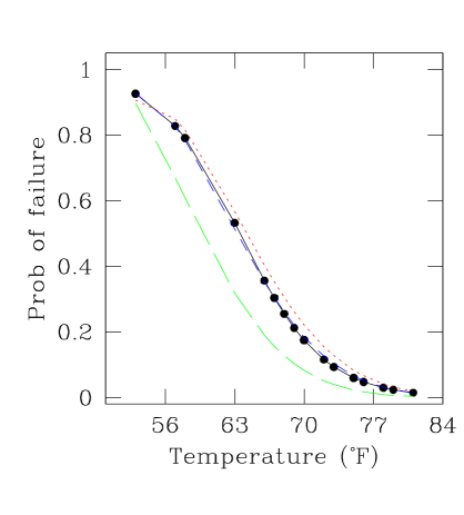
Figure 1: The solid black line shows failure probability variation $p_{mode}(T)$ with temperature $T$, as learnt using the modal values of the parameters of the logistic regression model considered by Robert and Casella (2004), given the O-ring data ${\bf D}$. The filled black circles represent $p_{mode}(t_{i})$, where $T=t_{i}$ is the temperature in the $i$-th row of the O-ring data, $i=1,\ldots,23$. Thee distinct SFN-shaped functions of $T$, that approximate $p_{mode}(T)$ differently, i.e. are differently distant from $p_{mode}(T)$, are depicted: $p_{blue}(T)$ in the broken (blue in the e-version) lines, $p_{red}(T)$ in dotted (red in the e-version) lines and $p_{green}(T)$ in the long-dashed (green in the e-version) lines.

Then $p_{mode}(T)$ is the variation in the failure probability with temperature that describes the measured data ${\bf D}$. We approximate $p_{mode}(T)$ with model function $p_{k}(T)$, where $k$ is a string-valued variable, $k=^{\prime\prime}red^{\prime\prime},``blue^{\prime\prime},``green^{\prime\prime}$, with the quality of the approximation parametrised by the constant mean square distance $\alpha_{k}$:

$$\alpha_{k}=\displaystyle{\frac{\sum\limits_{i=1}^{23}\left(p_{mode}(t_{i})-p_{k}(t_{i})\right)^{2}}{23}}.$$ (4.6)

The variation of failure probability with $T$, as displayed in Figure 1, reminds us of the shape of a (scaled) folded-normal density function (Leone et al., 1961). This motivates us to choose a scaled-folded-normal functional form for $p_{k}(T)$, as follows.

$$p_{k}(T)=s_{k}\displaystyle{\left[\exp\left(-\frac{(T-m_{k})^{2}}{2v_{k}}\right)+\exp\left(-\frac{(T+m_{k})^{2}}{2v_{k}}\right)\right]},$$ (4.7)

where the parameters of this function–the scaled-folded-normal (SFN) function–are: $S\in{\mathbb{R}}_{\geq 0}$, $M\in{\tau}\subset{\mathbb{R}}$ and $V\in{\mathbb{R}}_{\geq 0}$, which take values $s_{k},m_{k},v_{k}$ in the SFN-shaped variation $p_{k}(T)$ of failure probability with temperature. Thus, in the $k$-th model, the model parameter vector is $\boldsymbol{\theta}_{k}=(s_{k},m_{k},v_{k})^{T}$, $k=``red^{\prime\prime},``blue^{\prime\prime},``green^{\prime\prime}$. Table 1 includes the constant mean squared distance parameter, $\alpha_{k}$, that defines the SFN function $p_{k}(T)$, given $p_{mode}(T)$.

We want to test for the null $H_{0}^{(k)}$, given the O-ring data. Here $H_{0}^{(k)}$ states that the measurable $Y$–measurements of which comprise ${\bf D}$–is distributed as Bernoulli with probability for a “fail” that is an SFN-shaped function of $T$, namely $p_{k}(T)$, that approximates $p_{mode}(T)$ s.t. the mean squared distance between these two functions computed at $t_{1},\ldots,t_{23}$ is a constant $\alpha_{k}$, (presented in the 6-th column of Table 1). Then if at temperature $T=t$, the measurable is $Y=y$ (=1 or 0 for fail or not-fail, respectively), the $k$-th null is

$$H_{0}^{(k)}:\Pr(Y=y) = \left(p_{k}(t)\right)^{y}\left(1-p_{k}(t)\right)^{1-y},\quad\mbox{where}$$

$$p_{k}(T)\quad{\mbox{is an SFN function of $T$, s.t.}}, \displaystyle{\frac{\sum\limits_{i=1}^{23}\left(p_{mode}(t_{i})-p_{k}(t_{i})\right)^{2}}{23}}=\alpha_{k},$$ (4.8)

$k=^{\prime\prime}blue^{\prime\prime},\>^{\prime\prime}red^{\prime\prime},\>^{\prime\prime}green^{\prime\prime}$. Here the constant $\alpha_{blue}=0.00005657,\alpha_{red}=0.001411,\alpha_{green}=0.01234$ and $t_{i}$ is the temperature in the $i$-th row of the O-ring data. Thus, the $k$-th null is not sharp, for any $k$. By null $H_{0}^{(k)}$, the observed temperature variation of O-ring failure rate is described by $p_{k}(T)$, where ${p}_{k}(T)$ is known to be an approximation to $p_{mode}(T)$ with the quality of the approximation parametrised by the given distance $\alpha_{k}$ between them. Now, $p_{mode}(T)$ describes ${\bf D}$ well, as learnt by Robert and Casella (2004). Thus, the O-ring data is described approximately well by $p_{k}(T)$, where the quality of such an approximation is given by how well $p_{k}(T)$ approximates $p_{mode}(T)$, i.e. how small $\alpha_{k}$ is. Thus, the smaller the $\alpha_{k}$, the better does $p_{k}(T)$ describe the data ${\bf D}$, i.e. higher is the support in ${\bf D}$ for $H_{0}^{(k)}$. Then we expect high support in ${\bf D}$ for $H_{0}^{(blue)}$ as $\alpha_{blue}$ is small (smallest of the three models considered). On the other hand, owing to the higher value of $\alpha_{red}$, support in ${\bf D}$ for $H_{0}^{(red)}$ is expected to be less than for $H_{0}^{(blue)}$. Equally, support in ${\bf D}$ for $H_{0}^{(green)}$ is expected to be least, as $p_{green}(T)$ is the worst of the three approximations to $p_{mode}(T)$ (corroborated in Figure 1).

Values of $S,M,V$ that can define the SFN function $p_{k}(T)$ that approximates $p_{mode}(T)$ according to given distance $\alpha_{k}$, are tabulated in Table 1 for each $k$. This table also includes $\Pr(H_{0}^{(k)}|{\bf D})$, which is the support for the $k$-th null in the measured O-ring data ${\bf D}$ that comprises measured values of $Y$. The last column of this table gives the logarithm of the ratio $\Omega_{k}$ of the marginalised posterior of $\boldsymbol{\theta}_{k}$, given data ${\bf D}$ to the data ${\bf D}^{/}_{k}$ that is generated from the $k$-th model of thermal variation in the O-ring data (to be precise, ${\bf D}^{/}_{k}$ comprises 23 random numbers, the $i$-th of which is sampled from a Bernoulli distribution with rate $p_{k}(t_{i})$, $i=1,\ldots,23$).

Table 1:

k	SFN function used	$s_{k}$	$m_{k}$	$v_{k}$	$\alpha_{k}$	$\Pr(H_{0}^{(k)}|{\bf D})$	$\lg\left(\Omega_{k}\right)$
$red$	${p}_{red}(T)$	0.91	53.4	98.1	0.001411	0.8168	-1.0814
$blue$	${p}_{blue}(T)$	0.97	51.7	99.0	0.00005657	1	2.8893
$green$	${p}_{green}(T)$	1.02	48.0	96.5	0.01234	0	-8.5292

Here, the values of $\alpha_{k}$ are not arbitrarily chosen, but very much motivated by aspects of this application. $p_{blue}(T)$ is the least squares fit of an SFN-shaped function of $T$ to the sample $\{(t_{i},p_{mode}(t_{i}))\}_{i=1}^{23}$ taken from $p_{mode}(T)$ that is learnt by Robert and Casella (2004) (the filled black circles in Figure 1); $p_{bue}(T)$ is depicted in this figure in blue broken lines. The fit has a mean square error (MSE) of $\alpha_{blue}$ of about 0.00005657. Figure 1 also includes the SFN function ${p}_{red}(T)$ in dotted (red) lines. ${p}_{red}(T)$ is only a moderately good fit with an MSE of about 0.001411 (=$\alpha_{red}$). This SFN function $p_{red}(T)$ is parametrised by the modal values of $S$, $M$ and $V$ that are learnt using data ${\bf D}$ in an MCMC-based inference scheme. To achieve the modal values of $S,M,V$, we model $p(T)$ as an SFN function with unknown parameters $S,M,V$, so that the likelihood is rendered as in the RHS of Equation 4.5, except now $p_{i}$ is the value of the SFN function $p(T)$ computed at $T=t_{i}$. Using this likelihood and flat priors on all three unknown parameters, we generate posterior samples from $\pi(S,M,V|{\bf D})$ using Random-Walk Metropolis-Hastings. Let us refer to this MCMC chain as “Chain I” for future reference. The trace of this joint posterior probability in this chain is shown in Figure 3 in the solid black line. The marginals of $S$, $M$ and $V$ are shown in Figure 2. So when the modal values of these marginals are employed as $s_{red},m_{red}$ and $v_{red}$ (see columns 3,4,5 of Table 1), in an SFN function of $T$ (Equation 4.7), $p_{red}(T)$ results, which is $\alpha_{red}$ distance away from $p_{mode}(T)$. $p_{green}(T)$ is constructed by choosing a value of $S,M,V$ each from the tails of their respective marginals learnt using ${\bf D}$ (Figure 2). $p_{green}$ is a bad approximation of $p_{mode}(T)$, as parametrised by a high $\alpha_{green}$ (of about 0.01234).

Figure 2: Panels show marginals of the unknown parameters $S,M,V$ that parametrise an SFN function $p(T)$ that models the variation of failure probability with temperature $T$. These marginals are learnt using an MCMC chain, with the O-ring data.

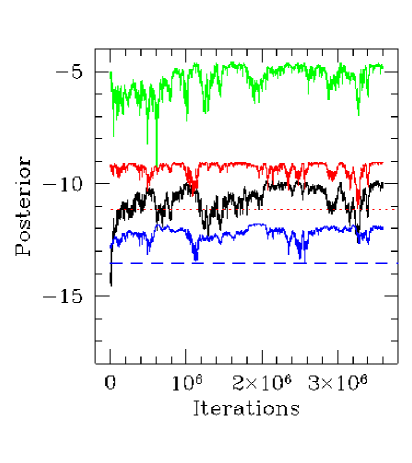
Figure 3: In solid black: trace of the joint posterior probability density $\pi(S,V,M|{\bf D})$ of the unknown model parameters $S,M,V$, given measured data ${\bf D}$, from the MCMC chain Chain I. In broken (blue) lines: trace of the posterior of $S,V,M$ given generated data ${\bf D}^{/}_{blue}$ that is randomly sampled from a Bernoulli distribution with rate given by the SFN function $p_{blue}(T)$. This chain corresponds to the lowest posterior values amongst the four chains shown here. $\pi^{(min)}(S,V,M|{\bf D}^{/}_{blue})$ is depicted in the broken (blue) lines. In dotted (red) lines: trace of $\pi(S,V,M|{\bf D}^{/}_{red})$ where ${\bf D}^{/}_{red}$ is generated using $p_{red}(T)$ as the variation in failure probability with $T$; minimum of this posterior is shown in (red) dots. In (green) long dashes: trace of $\pi(S,V,M|{\bf D}^{/}_{green})$ where ${\bf D}^{/}_{green}$ is generated using $p_{green}(T)$. This chain occurs at the highest posterior density values out of the four chains shown here.

The test is implemented using the following steps.

1. We consider the measurable $Y$ to be a Bernoulli variate with rate parameter that varies with temperature as $p(T)$–modelled as an SFN function with unknown model parameter vector $\boldsymbol{\theta}=(S,M,V)^{T}$. We perform Bayesian learning of these parameters given the measured data ${\bf D}$, in “Chain I”. $\pi(\boldsymbol{\theta}|{\bf D})$ is shown in Figure 3 in the solid black line.

2. We identify the benchmark model ${\cal M}_{k}$ in which the $k$-th null is true, $k=^{\prime\prime}red^{\prime\prime},``blue^{\prime\prime},``green^{\prime\prime}$. Then in model ${\cal M}_{k}$, the variation of failure probability with temperature is an SFN-shaped function $p_{k}(T)$, s.t. the mean squared distance between itself and $p_{mode}(T)$, computed at the temperature values in each row of the O-ring data, is $\alpha_{k}$. Such a function $p_{k}(T)$ is achieved using $\boldsymbol{\theta}_{k}$ that is given in Table 1. Then we attain the generated data ${\bf D}^{/}_{k}$ by selecting a random Bernoulli variate with rate given by this $p_{k}(T)$. We then run an MCMC chain with ${\bf D}^{/}_{k}$, to obtain samples from $\pi(\boldsymbol{\theta}|{\bf D^{/}}_{k})$. (This chain is of course different from “Chain I” that is run with data ${\bf D}$). We employ this chain to identify the minimum value of $\pi(\boldsymbol{\theta}|{\bf D^{/}}_{k})$. Trace of the posterior in this chain is shown in Figure 3 in (colour $k$ in the electronic version) dashed lines for $k=^{\prime\prime}blue^{\prime\prime}$, dotted lines for $k=^{\prime\prime}red^{\prime\prime}$, broad-dashed lines for $k=^{\prime\prime}green^{\prime\prime}$. The minimum posterior in the post-burnin part of the chain is also presented in the figure as a horizontal line in the corresponding line-type.

3. Next we identify the sub-space ${\cal T}_{{\cal M}_{k}}({\bf D})$ that is the native space of those model parameter vectors, for which $\pi(\boldsymbol{\theta}|{\bf D})$ equals or exceeds the minimum posterior attained under the $k$-th null, i.e. when $p_{mode}(T)$ is approximated by $p_{k}(T)$, within a distance parameter of $\alpha_{k}$. Once we identify this sub-space, we then need to compute $\Pr(\boldsymbol{\theta}\in T_{{\cal M}_{k}}|{\bf D})=\displaystyle{\int\limits_{\boldsymbol{\theta}\in{\cal T}_{{\cal M}_{k}}({\bf D})}\pi(\boldsymbol{\theta}|{\bf D})d\boldsymbol{\theta}}$. However, we avoid the computation of this integral, and instead approximate the probability of membership in this sub-space via a simple case-counting scheme. Thus, we identify the number $P_{k}$ out of the total of $Q_{k}$ $\boldsymbol{\theta}$ samples that are generated in the MCMC chain “Chain I”, run with measured data ${\bf D}$, for which posterior probability exceeds, or is equal to $\pi^{(min)}(\boldsymbol{\theta}|{\bf D^{/}}_{k})$. Then, $\Pr(\boldsymbol{\theta}\in T_{{\cal M}_{k}}|{\bf D})$ is approximated by $\displaystyle{\frac{P_{k}}{Q_{k}}}$. Then by Equation 4.2, the probability of the $k$-th null conditional on the measured data, is $\Pr(\boldsymbol{\theta}\in T_{{\cal M}_{k}}|{\bf D})\approx\displaystyle{\frac{P_{k}}{Q_{k}}}$. This is tabulated in the 7-th column of Table 1 for each $k=^{\prime\prime}red^{\prime\prime},``blue^{\prime\prime},``green^{\prime\prime}$. The 8-th column contains the logarithm of the odds ratio $\Omega_{k}$ discussed in Equation 4.1.

As said above in the paragraph following Equation 4.8, we expect high support in ${\bf D}$ for $H_{0}^{(blue)}$. In fact, in the chain run with generated data ${\bf D}^{/}_{blue}$, $\pi^{(min)}(\boldsymbol{\theta}|{\bf D^{/}}_{blue})$ is about -13.55, which is lower than $\pi(\boldsymbol{\theta}|{\bf D})$ obtained for all $\theta$ samples generated in Chain I (in solid black line in Figure 3), i.e. $\displaystyle{\frac{P_{blue}}{Q_{blue}}}\approx\Pr(\boldsymbol{\theta}\in T_{{\cal M}_{blue}}|{\bf D})=\Pr(H_{0}^{(blue)}|{\bf D})=1$–the highest support possible in the measured data. Compared to $H_{0}^{(blue)}$, support in ${\bf D}$ for $H_{0}^{(red)}$ is expected to be less. Indeed we find that $\displaystyle{\frac{P_{red}}{Q_{red}}}\approx 0.8168$ or equivalently, $\Pr(\boldsymbol{\theta}\in T_{{\cal M}_{red}}|{\bf D})=\Pr(H_{0}^{(red)}|{\bf D})$ is about 0.8168. Here $\pi^{(min)}(\boldsymbol{\theta}|{\bf D^{/}}_{red})\approx-11.14$. For the crudest (out of the three models) approximation for $p_{mode}(T)$, in the chain run with generated data ${\bf D}^{/}_{green}$, the minimum posterior probability exceeds the posterior achieved for every $\boldsymbol{\theta}$ sample generated in Chain I that is run with measured data ${\bf D}$. Then fraction of these samples for which posterior exceeds of equals posterior achieved in chain run with generated data, is 0, i.e. $\displaystyle{\frac{P_{green}}{Q_{green}}}=0$ implying $\Pr(H_{0}^{(green)}|{\bf D})=0$.

As in this application we are not comparing support in one data set for a given null, to support in another data for a different null, we could have computed the support in the measured O-ring data ${\bf D}$, for the $k$-th null, using the ratio of the marginalised posterior given ${\bf D}$ to that given ${\bf D}^{/}$ that is defined in Equation 4.1 as $\Omega_{k}$. In this example, we can perform posterior computation given measured and generated data; $\int\limits_{\boldsymbol{\theta}}\pi(\boldsymbol{\theta}|{\bf D})$ is about $5.4\times 10^{-10}$, and $\int\limits_{\boldsymbol{\theta}}\pi(\boldsymbol{\theta}|{\bf D}^{/}_{k})$ is about $2.7\times 10^{-6}$, $1.6\times 10^{-9}$, $3.0\times 10^{-11}$, for $k=^{\prime\prime}green^{\prime\prime},``red^{\prime\prime},``blue^{\prime\prime}$, so that support in ${\bf D}$ for the $k$-th model as in $\log(\Omega_{k})$, is about -8.53, -1.08, 2.89 for $k=^{\prime\prime}green^{\prime\prime},``red^{\prime\prime},``blue^{\prime\prime}$ respectively (see Table 1).

5 Implementation of the new test to the galactic application

Following Section 4, we implement the new test by finding the minimum posterior achieved under the null, in order to identify the sub-space ${\cal T}_{{\cal M}_{i}}({\bf D}_{i})$, and then proceed to compute the probability of the null given data ${\bf D}_{i}$, as the probability that $\boldsymbol{\theta}_{i}\in{\cal T}_{{\cal M}_{i}}({\bf D}_{i})$.

Let the model parameter vector that minimises the posterior probability density under the null, be referred to as $\boldsymbol{\theta}_{i}^{(min)}$.

5.1 Identification of posterior-optimising model parameter vector, under the null

In order to identify the vector, $\boldsymbol{\theta}_{i}^{(min)}$, the following scheme is used, where the scheme below is expressed in the paradigm of the Bayesian method in which the discretised state space density vector ${\boldsymbol{\Psi}}^{(i)}$ and the discretised gravitational mass density vector $\boldsymbol{\rho}^{(i)}$ are learnt given the measured data ${\bf D}_{i}$, under the assumption that the state space $pdf$ is isotropic (see Section 3.1). The benchmark model ${\cal M}_{i}$ is such, that under it, the state space $pdf$ is an isotropic function of the location $\boldsymbol{X}$ and velocity $\boldsymbol{V}$ of a galactic particle, i.e. the null $H_{0}^{(i)}$ is true in model ${\cal M}_{i}$.

• We perform inference on $\boldsymbol{\theta}_{i}$ given measured data ${\bf D}_{i}$, with Metropolis-Hastings. During this inference, let the state space vector in the $c$-th iteration be $\boldsymbol{\theta}_{i}^{(c)}$, $c=1,\ldots,N_{0}$, where the chain is $N_{0}$ steps long. Upon convergence, the unknown $\boldsymbol{\theta}_{i}$, i.e. ${\boldsymbol{\Psi}}_{i}$ and ${\boldsymbol{\rho}}_{i}$ in our application, are learnt within 95$\%$ HPD credible regions. From a given chain, we identify the modal parameter vector $\boldsymbol{\theta}_{i}^{(M)}:=(\Psi_{1}^{(M,i)},\ldots,\Psi_{N_{E}}^{(M,i)},\rho_{1}^{(M,i)},\rho_{N_{x}}^{(M,i)})^{T}$, corresponding to the mode of the posterior density $\pi(\boldsymbol{\theta}_{i}|{\bf D}_{i})$.

• We learn the discretised state space density ${\boldsymbol{\Psi}}^{(M,i)}$ and gravitational mass density $\boldsymbol{\rho}^{(M,i)}$ given ${\bf D}_{i}$, in the aforementioned Bayesian method, where the learnt state space density is isotropic by construct, (since isotropy of the state space density is the basic underlying assumption of the Bayesian method). From this learnt isotropic $pdf$, at the learnt $\boldsymbol{\rho}^{(M,i)}$, we simulate an $N_{data}^{(i)}$-sized data set of the observed variables $X_{1}$, $X_{2}$ and $V_{3}$. Let this generated data set be
  

  $${\bf D}_{i}^{(gen)}:=\{(x_{1,\>gen}^{(k)},x_{2,\>gen}^{(k)},v_{3,\>gen}^{(k)})\}_{k=1}^{N_{data}^{(i)}},$$

  where the size of ${\bf D}_{i}$ is $N_{data}^{(i)}$.

• Importantly, generated data ${\bf D}_{i}^{(gen)}$ is simulated from an isotropic state space function (the discretised form of which is) ${\boldsymbol{\Psi}}^{(M,i)}$, at ${\boldsymbol{\rho}}^{(M,i)}$, using rejection sampling, according to the following algorithm.

  1. We solve for the function $\Phi(X)$ that relates to the sought unknown $\rho(X)$ via the Poisson equation: $\nabla^{2}\Phi(X)=-4\pi G\rho(X)$, where $X:=\parallel\boldsymbol{X}\parallel$. The relevance of $\Phi(X)$ is that it is part of the function $E(X,V)$ ($=\Phi(X)+\eta(V)$) that was introduced in Section 3.1, where the function $E(\cdot,\cdot)$ forms the argument of state space density: $\Psi_{i}(E(X,V))$. By its dependence on $X$ and $V$, (via $E(X,V)$), this model of the state space $pdf$ is an isotropic function of $\boldsymbol{X}$ and $\boldsymbol{V}$ (see Section 3.1). Then isotropic state space $pdf$ bears the form $\Psi_{i}(E(X,V))$ orequivalently, the form $\Psi_{i}(\Phi(X),\eta(V))$ which is again equivalent in form to $\Psi_{i}(\rho(X),\eta(V))$, by invoking Poisson equation. In this way, the discretised version $\boldsymbol{\rho}$, of $\rho(X)$, can be embedded into the argument of the state space density that is modelled as isotropic; $\boldsymbol{\rho}$ thereby enters the likelihood of the unknowns given the data, thus allowing for inference on the unknown $\boldsymbol{\rho}$.

  2. In our application, $E(X,V)$ is identified with the total energy of a galactic particle, with $\Phi(X)$ the potential and $\eta(V)=V^{2}/2$ identified with the kinetic energy. In fact in our application, $\Phi(X)\leq 0$ for $\rho(X)\geq 0$ and the minimum value of $\Phi(X)$ is $\Phi(0)$. We consider only those galactic particles that are bound to the galaxy; the energy of any such bound particle is negative. Thus, in this application, $E(X,V)$ can at most approach 0, and at least be $\Phi(0)$. Thus, the value $\epsilon$ of $E(X,V)$ normalised by $\Phi(0)$, lies in (0,1].

  3. Since the value of $E(X,V)\>(=\Phi(X)+V^{2}/2)$ is minimally $\Phi(0)$, and maximally approaches 0, the range of values of $V$ is $[-\sqrt{-2\Phi(0)},\sqrt{-2\Phi(0)}]$.

  4. We discretise $\rho(X)$ by discretising the range that $x$ lies in, and discretise $\Psi(E)$ by discretising the range that $\epsilon$ lies in. Thus, $\rho_{p}=\rho(x)$ if $x\in[(p-1)\delta,p\delta)$ and $\Psi_{t}=\Psi(\epsilon)$ if $\epsilon\in[(t-1)\delta_{E},t\delta_{E})$, for $p=1,\ldots,N_{x}$, $t=1,\ldots,N_{E}$. (Though we use uniform binning in this application–with constant bin widths $\delta>0$ and $\delta_{E}>0$–other forms of discretisation can be potentially implemented within this scheme).

  5. We compute $\Phi(x)$ via $M(x)$ where $\displaystyle{\Phi(x)=\frac{-GM(x)}{x}}$ with $M(x)=\displaystyle{\int_{s=0}^{x}4\pi\rho(s)s^{2}ds}$ and $G$ is a known (Universal Gravitational) constant. For computational ease we discretise this integral, to define

     $$M(x) = \displaystyle{\sum_{q=1}^{p}\frac{4\pi}{3}[q^{3}\delta^{3}-(q-1)^{3}\delta^{3}]\rho_{q}+\frac{4\pi}{3}[x^{3}-p^{3}\delta^{3}]\rho_{p+1}},\quad{\textrm{for}}\quad x\in[p\delta,(p+1)\delta),$$

     $$M(x) = \displaystyle{\sum_{q=1}^{N_{x}}\frac{4\pi}{3}[q^{3}\delta^{3}-(q-1)^{3}\delta^{3}]\rho_{q}}\quad{\textrm{for}}\quad x\geq N_{x}\delta,$$

     $$M(x) = \displaystyle{\frac{4\pi}{3}[x^{3}]\rho_{1}}\quad{\textrm{for}}\quad 0\leq x\leq\delta.$$

     Here $N_{x}\delta$ is the maximum radius to which data are available and $\rho_{q}$ is the gravitational mass density in the $q$-th radial bin. This defines $\Phi(x)$ for any $x\geq 0$, given the identified ${\boldsymbol{\rho}}^{(M,i)}$.

  6. Next, we sample $\epsilon$, i.e. the value of $E(\cdot,\cdot)$ normalised by $\Phi(0)$. As $\epsilon\in(0,1]$, we choose $\epsilon$ randomly from ${\cal U}[0,1]$, where ${\cal U}[a,b]$ is the uniform distribution over the range $[a,b]$, $a,b\in{\mathbb{R}}$. Let the sampled $\epsilon$ be such that it lies in the $t$-th energy bin, i.e. $\epsilon\in[(t-1)\delta_{E},t\delta_{E}]$, $t=1,\ldots,N_{E}$; let the $t$-th component of ${\boldsymbol{\Psi}}^{(M,i)}$ be $\Psi_{t}^{(M,i)}$.

  7. The 3 components of the location vector are continuous in $[-N_{x}\delta,N_{x}\delta]$. So we sample, $X_{1},X_{2},X_{3}\sim{\cal U}[-N_{x}\delta,N_{x}\delta]$ and using these sampled values $x_{1},x_{2},x_{3}$, obtain the value of $\parallel\boldsymbol{x}\parallel\equiv x=\sqrt{x_{1}^{2}+x_{2}^{2}+x_{3}^{2}}$. Let $x$ be such that it lies in the $q$-th radial bin, i.e. $x\in[(q-1)\delta,q\delta]$, $q=1,\ldots,N_{x}$. For this chosen $x$, we then compute $\Phi(x)$ using $M(x)$ from Equation LABEL:eqn:phi and the definition $\displaystyle{\Phi(x)=\frac{-GM(x)}{x}}$. We normalise $\Phi(x)$ by $\Phi(0)$, so that $\Phi(x)$ now lives in the range $(0,1]$.

  8. Check if the chosen $\epsilon>\Phi(x)$. If not, go back to step number 6. If yes, then recall that the components of the velocity vector, $V_{1}$, $V_{2}$, $V_{3}$ is each continuous in $[-\sqrt{-2\Phi(0)},\sqrt{-2\Phi(0)}]$, to suggest that $V_{1},V_{2},V_{3}$ be each sampled as $V_{1},V_{2},V_{3}\sim{\cal U}[-\sqrt{-2\Phi(0)},\sqrt{-2\Phi(0)}]$. So we draw $v_{1},v_{2},v_{3}$ individually from this uniform distribution.

  9. In this step, we sample from $\Psi_{t}^{(M,i)}$ using rejection sampling. Here the chosen $\epsilon$ is in the $t$-th energy-bin so that $\Psi_{t}^{(M,i)}$ is the value of the state space $pdf$ in our discretised model. The rejection sampling is done by checking if $\displaystyle{\frac{\Psi_{t}^{(M,i)}}{g(\epsilon)}}>u$ or not, where $u$ is a random number in $[0,1]$, $u\sim{\cal U}[0,1]$. Here $g(\epsilon)$ is the proposal density function that is chosen to envelope over $\Psi(\epsilon)$, $\forall\epsilon$, and is defined as $g(\epsilon)=1.05\forall\epsilon$. This is an adequate choice because the state space $pdf$ $\Psi(\epsilon)$ is normalised to be in $(0,1]$. If the above inequality holds, we allow an integer-valued flag, $\gamma$, an increment of 1 and accept the values $x_{1},x_{2}$ and $v_{3}$ as chosen in steps 7 and 8 respectively, as the $\gamma$-th data point in ${\bf D}_{i}^{(gen)}$. We iterate over points 4 to 9, until $\gamma$ equals $N_{data}^{(i)}$.

• Now that we have discussed the algorithm used to sample the generated data ${\bf D}_{i}^{(gen)}$, in order to estimate $\boldsymbol{\theta}_{i}$ using this generated data, we start a new MCMC chain. We remind ourselves that unlike the measured data ${\bf D}_{i}$ that may live in an anisotropic state space, the generated data ${\bf D}_{i}^{(gen)}$ is sampled from an isotropic state space density (rather its discretised form $\boldsymbol{\Psi}_{i})$, i.e. posterior of $\boldsymbol{\theta}_{i}$ given data ${\bf D}_{i}^{(gen)}$ is the posterior when the null is true. Post burn-in, samples of $\boldsymbol{\theta}_{i}$ vectors generated in each iteration are recorded. In this recorded sample of values of $\boldsymbol{\theta}_{i}$, that which minimises the posterior density $[\Psi_{1}^{(i)},\ldots,\Psi_{N_{E}}^{(i)},\rho_{1}^{(i)},\ldots,\rho_{N_{x}}^{(i)}|{\bf D}_{i}^{(gen)}]$, is the posterior-minimising parameter in the benchmark model ${\cal M}_{i}$:

  $$\boldsymbol{\theta}_{i}^{(min)}:=(\Psi_{1}^{(i,min)},\ldots,\Psi_{N_{E}}^{(i,min)},\rho_{1}^{(i,min)},\ldots,\rho_{N_{x}}^{(i,min)})^{T}.$$ (5.2)

  Let the minimum posterior of $\boldsymbol{\theta}$ given the generated data be $\pi^{(min)}(\boldsymbol{\theta}_{i}|{\bf D}_{i}^{(gen)})$.

5.2 Probability of membership in subspace ${\cal T}_{{\cal M}_{i}}({\bf D}_{i})$

We need to identify the sub-space ${\cal T}_{{\cal M}_{i}}({\bf D}_{i})$ in which live model parameter vectors, the posterior of which equals or exceeds the minimal posterior probability density attained under the null, i.e. $\pi^{(min)}(\boldsymbol{\theta}_{i}|{\bf D}_{i}^{(gen)})$. We are required to integrate the posterior probability density of $\boldsymbol{\theta}_{i}$ given measured data ${\bf D}_{i}$, over all such values of $\boldsymbol{\theta}_{i}$ that live in the subspace ${\cal T}_{{\cal M}_{i}}({\bf D}_{i})$, i.e. compute $\displaystyle{\int\limits_{\boldsymbol{\theta}_{i}\in{\cal T}_{{\cal M}_{i}}({\bf D}_{i})}\pi(\boldsymbol{\theta}_{i}|{\bf D}_{i})d\boldsymbol{\theta}_{i}}$. This integral is then equal to $\Pr(\boldsymbol{\theta}\in T_{{\cal M}_{i}}|{\bf D}_{i})$.

Thus, in this approach, it is possible to implement $\Pr(H_{0}^{(i)}|{\bf D}_{i})$, even in a high-dimensional state space, by approximating this probability of membership of the model parameter vector $\boldsymbol{\theta}_{i}$ in ${\cal T}_{{\cal M}_{i}}({\bf D}_{i})$, with a case-counting scheme. In other words, we compute the proportion of the model parameter vectors for which $\pi^{(min)}(\boldsymbol{\theta}_{i}|{\bf D}_{i}^{(gen)})\leq\pi(\boldsymbol{\theta}_{i}|{\bf D}_{i})$, as recovered in the post-burnin stage of chains run with measured data ${\bf D}_{i}$.

Thus, let there be a total of $Q_{i}$ number of samples of $\boldsymbol{\theta}_{i}$ vectors recovered in the post-burnin stage in chains run with measured data ${\bf D}_{i}$. Out of these, let $P_{i}$ number of $\boldsymbol{\theta}_{i}$ vectors be such that $\pi^{(min)}(\boldsymbol{\theta}_{i}|{\bf D}_{i}^{(gen)})\leq\pi(\boldsymbol{\theta}_{i}|{\bf D}_{i})$. Here, $Q_{i},\;P_{i}\in{\mathbb{Z}}_{+}$, $P_{i}\leq Q_{i}$. Then the fraction $P_{i}/Q_{i}$ is an approximation to the probability that $\boldsymbol{\theta}_{i}\in{\cal T}_{\cal M_{i}}({\bf D}_{i})$. Then recalling Equation 4.2, we state that

$$\Pr({H_{0}^{(i)}}|{\bf D}_{i})=\displaystyle{\frac{P_{i}}{Q_{i}}},$$ (5.3)

$i$=1,2.

6 Testing with synthetic galactic data

In this section, we implement this new test to find the probability of the null (that the state space of a toy galaxy is isotropic), given the (simulated) data at hand. For this simulation exercise, we use synthetic data that is sampled from chosen state space density models, constructed to simulate real galactic state space density functions. To be precise, we sample data sets ${\bf D}_{A}$ and ${\bf D}_{B}$ from two chosen state space density functions $f_{A}^{(True)}(\boldsymbol{X},\boldsymbol{V})$ and $f_{B}^{(True)}(\boldsymbol{X},\boldsymbol{V})$ respectively, that are anisotropic to different extents, as parametrised by an anisotropy parameter that we discuss below. We realise that a state space density that is a function of $\boldsymbol{X}$ and $\boldsymbol{V}$ via a function such as $E(X,V)$, is an isotropic function of vectors $\boldsymbol{X}$ and $\boldsymbol{V}$. On the other hand, a density function that depends on $\boldsymbol{X}$ and $\boldsymbol{V}$ via any form of these vectors, other than their $L^{2}$-norm, is not an isotropic function of $\boldsymbol{X}$ and $\boldsymbol{V}$.

The model state space $pdf$ that we sample the synthetic data ${\bf D}_{A}$ and ${\bf D}_{B}$ from, are

$$f_{\cdot}^{(True)}({\bf x},{\bf v}) = \displaystyle{\frac{1}{\sqrt{2\pi}\sigma}\exp\left(\frac{\epsilon(x,v)}{2\sigma^{2}}\right)\exp\left(-\frac{[P(\boldsymbol{x},\boldsymbol{v})]^{2}}{r_{a}^{2}\sigma^{2}}\right)}$$ (6.1)

$${\mbox{where}}\quad\epsilon(x,v) = \displaystyle{\frac{{{v}^{2}}/{2}+\Phi(x)}{\Phi_{0}}},$$ (6.2)

$${\mbox{and}}\quad[P(\boldsymbol{x},\boldsymbol{v})]^{2} = (x_{2}v_{3}-x_{3}v_{2})^{2}+(x_{3}v_{1}-x_{1}v_{3})^{2}+(x_{1}v_{2}-x_{2}v_{1})^{2},$$ (6.3)

and $r_{a}$ and $\sigma$ are parameters of this density. The first exponential term in the RHS of Equation 6.1 manifests the purely isotropic dependence on $\boldsymbol{X}$ and $\boldsymbol{V}$, while the second exponential term manifests dependence on $\boldsymbol{X}$ and $\boldsymbol{V}$ via a form that is different from the $L^{2}$-norm of these vectors, i.e. this second exponential term manifests anisotropic dependence on $\boldsymbol{X}$ and $\boldsymbol{V}$. Thus, the chosen state space density functions of the type in Equation 6.1, are anisotropic in general, with the strength of the (anisotropic) second exponential factor on the RHS of Equation 6.1, parametrised by the parameter $r_{a}$; the bigger is the value of $r_{a}$, higher is the relative amplitude of the anisotropic factor to the isotropic factor (that is parametrised only by $\sigma$). Equally, for $r_{a}$ approaching 0, the constructed state space $pdf$ in Equation 6.1 approaches an isotropic form. The parameter $r_{a}$ is then the anisotropy scale length. It is measured in the astronomical unit of length on galactic scales: “kiloparsec”, abbreviated to “kpc”.

We choose $f_{A}^{(True)}(\boldsymbol{X},\boldsymbol{V})$ to be more anisotropic than $f_{B}^{(True)}(\boldsymbol{X},\boldsymbol{V})$ by choosing $r_{a}$=4 kpc and $r_{a}$=0.2 kpc in the two models respectively. In every other way, inputs to $f_{A}(\boldsymbol{X},\boldsymbol{V})$ and $f_{B}(\boldsymbol{X},\boldsymbol{V})$ are identical. We choose $\sigma=220$, in units of km s^-1. To define $E(X,V)$ and thereby its value $\epsilon$ in Equation 6.1, we need to choose the form of $\Phi(X)$. We construct this to be

$$\Phi(x)=\displaystyle{-\frac{GM_{0}}{\sqrt{r_{c}^{2}+x^{2}}}},$$ (6.4)

where we chose the parameters to be $M_{0}=4\times 10^{11}$ times the mass of the Sun or “$M_{\odot}$” (astronomical unit of mass on galactic scales) and $r_{c}$=8 kpc. $G$ is a known physical constant, (the Universal Gravitational constant).

Having constructed $f_{A}^{(True)}(\boldsymbol{X},\boldsymbol{V})$ and $f_{B}^{(True)}(\boldsymbol{X},\boldsymbol{V})$, we simulate data ${\bf D}_{A}$ and ${\bf D}_{B}$ respectively from these state space densities, where each data set contains information on $X_{1}$, $X_{2}$ and $V_{3}$. Size of ${\bf D}_{A}$ is 710 while size of ${\bf D}_{B}$ is 135. The sampled $V_{3}$ data is chosen to be characterised by Gaussian noise $\sim{\cal N}(0,20^{2})$ which is typical of real-life galaxies that are nearby (Douglas et al., 2007).

The $i$-th null states that the data ${\bf D}_{i}$ is sampled from an isotropic state space density $f_{i}(\boldsymbol{X},\boldsymbol{V})$ for $i=A,B$, i.e. $f_{i}(\boldsymbol{X},\boldsymbol{V})=\Psi_{i}(E(X,V))$, $\Psi_{i}(\cdot)\geq 0$, where $X\in{\cal X}\subseteq{\mathbb{R}}_{\geq 0}$ and $V\in{\cal V}\subseteq{\mathbb{R}}_{\geq 0}$. To condense,

$$H_{0}^{(i)}:f_{i}(\boldsymbol{X},\boldsymbol{V})=\Psi_{i}(E(X,V)),\>\>\Psi_{i}(\cdot)\geq 0,$$ (6.5)

for $i=A,B$. When the null is true, the state space $pdf$ is an isotropic function of $\boldsymbol{X}$ and $\boldsymbol{V}$. As discussed above for our application, the intractability of the more complex model (anisotropic state space $pdf$) compels us to learn the model parameter $\boldsymbol{\theta}_{i}$ only under the null model, i.e. by assuming the state space to be isotropic. The model parameter vector for $i=A$ is $\boldsymbol{\theta}_{A}=(\Psi_{1}^{(A)},\ldots,\Psi_{N_{E}}^{(A)},\rho_{1}^{(A)},\ldots,\rho_{N_{x}}^{(A)})^{T}$ is learnt using data ${\bf D}_{A}$ under the assumption that the galactic state space is isotropic, where $\boldsymbol{\rho}_{A}:=(\rho_{1}^{(A)},\ldots,\rho_{N_{x}}^{(A)})^{T}$ and ${\boldsymbol{\Psi}}_{A}:=(\Psi_{1}^{(A)},\ldots,\Psi_{N_{E}}^{(A)})^{T}$. Similarly, we define $\boldsymbol{\theta}_{B}$, $\boldsymbol{\rho}_{B}$, $\boldsymbol{\Psi}_{B}$, learnt using data ${\bf D}_{B}$, while assuming an isotropic galactic state space.

In Figure 4 we present the posterior probability density $\pi(\boldsymbol{\theta}_{A}|{\bf D}_{A})$ (right panel) and $\pi(\boldsymbol{\theta}_{B}|{\bf D}_{B})$ (left panel), in grey (or red in the electronic version). The posterior probability density attained under the null, i.e. computed given the generated data, is shown in black in each case: $\pi(\boldsymbol{\theta}_{A}|{\bf D}_{A}^{(gen)})$ in the right and $\pi(\boldsymbol{\theta}_{B}|{\bf D}_{B}^{(gen)})$ in the left panel. We recall that the generated data sets ${\bf D}_{i}^{(gen)}$ are generated using rejection sampling from $\Psi_{i}(E)$–or rather its discretised version $\boldsymbol{\Psi}_{i}$ that is learnt using available measurements ${\bf D}_{i}$–at the estimated $\boldsymbol{\rho}_{i}$. See Section 5 for details of implementation of this rejection sampling.

It is clear that for the case of the more anisotropic true state space density, i.e. for case $A$, the posterior probability density of the model parameter vector falls below the minimal value of the posterior under the null, i.e. $\pi(\boldsymbol{\theta}_{A}|{\bf D}_{A})<\pi^{(min)}(\boldsymbol{\theta}_{A}|{\bf D}_{A}^{(gen)}),\>\forall\boldsymbol{\theta}_{A}$, implying that the sub-space ${\cal T}_{{\cal M}_{A}}({\bf D}_{A})$ is empty. It then follows that $\Pr(H_{0}^{(A)}|{\bf D}_{A})=0$, so that we reject null $H_{0}^{(A)}$ with 100$\%$ probability. In other words, the hypothesis that the data ${\bf D}_{A}$ is sampled from an isotropic state space density is rejected at probability of 1. This is indeed what we expect given that the true density $f_{A}^{(True)}(\boldsymbol{X},\boldsymbol{V})$ that ${\bf D}_{A}$ is sampled from is chosen to be strongly anisotropic.

For the case of the less anisotropic true state space density, i.e. for case $B$, in the post-burnin part of the chain (beyond the 600,000-th iteration; in black in Figure 4), $\pi^{(min)}(\boldsymbol{\theta}_{B}|{\bf D}_{B}^{(gen)})$ is depicted in the solid black line. There are multiple values of $\pi(\boldsymbol{\theta}_{B}|{\bf D}_{B})$ that exceed this minimal posterior achieved under the null. In fact, in the post-burnin stage of the chain run with data ${\bf D}_{B}$, $\pi(\boldsymbol{\theta}_{B}|{\bf D}_{B})\geq\pi^{(min)}(\boldsymbol{\theta}_{B}|{\bf D}_{B}^{(gen)})$ for 83,780 samples of $\boldsymbol{\theta}_{B}$ where there are 200,000 iterations, post-burnin in the chain. Thus, for this case, $\Pr({\cal T}_{{\cal M}_{B}}|{\bf D}_{B})=\displaystyle{\frac{87650}{200000}}\approx 0.5394$, i.e. the support against the null $H_{0}^{(B)}$ is 1-0.5394= 0.4606. Thus, the hypothesis that the data ${\bf D}_{B}$ is sampled from an isotropic state space density is rejected at probability 0.4606, given data ${\bf D}_{B}$.

This corroborates the strength of our test as we chose to sample data ${\bf D}_{B}$ from the true state space density $\Psi_{B}(\boldsymbol{X},\boldsymbol{V})$ that is constructed as mildly anisotropic, compared to the strongly anisotropic true density $\Psi_{A}(\boldsymbol{X},\boldsymbol{V})$ that data ${\bf D}_{A}$ is sampled from.

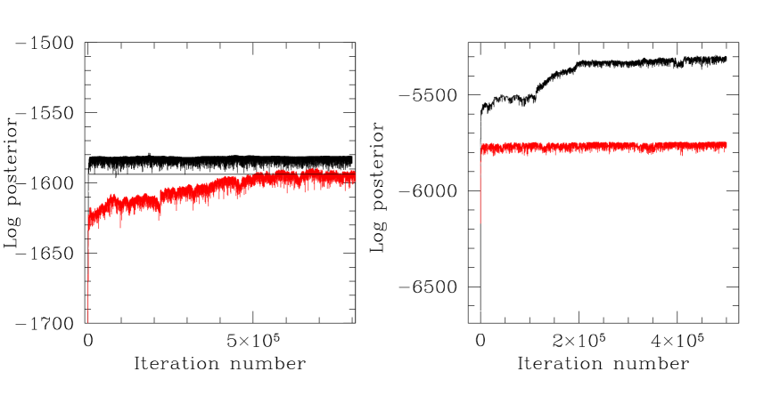
Figure 4: Figure showing log of the posterior probability density $\pi({\boldsymbol{\theta}}_{A}|{\bf D}_{A})$ (right) and $\pi({\boldsymbol{\theta}}_{B}|{\bf D}_{B})$ (left), in grey (or red in the electronic version), for chains that were run for 8$\times$10⁵ and 5$\times$10⁵ iterations respectively. The log of the posterior probability density of $\boldsymbol{\theta}_{A}$ and $\boldsymbol{\theta}_{B}$, given generated data ${\bf D}_{A}^{(gen)}$ and ${\bf D}_{B}^{(gen)}$ respectively, represent the posterior densities of the model parameters in the benchmark models in which the null is true; the traces of these posteriori are shown in black in the right and left panels. Here simulated data set ${\bf D}_{A}$ is about 5.3 times bigger in size than data ${\bf D}_{B}$. ${\bf D}_{A}$ is sampled from a true state space density that is constructed as strongly anisotropic, as distinguished from the mildly anisotropic true state space density that simulated data ${\bf D}_{B}$ is sampled from. In the right panel, the minimum value of the posterior when the null $H_{0}^{(A)}$ is true, is in excess of the posterior $\pi(\boldsymbol{\theta}_{A}|{\bf D}_{A})$ at all iterations, i.e. for no value of $\boldsymbol{\theta}_{A}$ does $\pi(\boldsymbol{\theta}_{A}|{\bf D}_{A})\geq\pi(\boldsymbol{\theta}_{A}|{\bf D}_{A}^{(gen)})$. Thus, the null $H_{0}^{(A)}$ is rejected at a probability of 1. On the other hand, from the post-burnin part of the chain (beyond the 600,000-th iteration) we find that the minimum value of the posterior under the benchmark model ${\cal M}_{B}$ (shown in the black solid line) falls short of $\pi(\boldsymbol{\theta}_{B}|{\bf D}_{B})$ at 87,650 number of iterations, out of the 200,000 samples of $\boldsymbol{\theta}_{B}$ generated in the post-burnin part of the chain run with ${\bf D}_{B}$. The null $H_{0}^{(B)}$ is then rejected at a probability of 1 - 87650/200,000 $\approx$ 0.4606.

Table 2: Table displaying conditional probability of null $H_{0}^{(i)}$ (Statement 6.5) given synthetic data ${\bf D}_{i}$ that is simulated from true anisotropic state space density $f_{i}^{(True)}(\boldsymbol{X},\boldsymbol{V})$, where the density for $i=A$ is more anisotropic than for $i=B$. Column 2 shows the value $r_{a}$ of the anisotropy parameter that parametrises the deviation of $f_{i}^{(True)}(\boldsymbol{X},\boldsymbol{V})$ from an isotropic function of $\boldsymbol{X}$ and $\boldsymbol{V}$. Column 3 shows the number $P_{i}$ of generated samples of $\boldsymbol{\theta}_{i}$ for which the posterior probability density given data ${\bf D}_{i}$, exceeds the minimum values of the posterior density under the null; column 4 gives the total number $Q_{i}$ of samples of $\boldsymbol{\theta}_{i}$ generated in the chain. The ratio of the entries in Column 3 to that in Column 4 is in Column 5–it is taken to approximate $\Pr(\boldsymbol{\theta}_{i}\in{\cal T}_{{\cal M}_{i}}({\bf D}_{i}))$ which in turn is equal to $\Pr(H_{0}^{(i)}|{\bf D}_{i})$ (see Equation 4.4 and Equation 4.2). Column 6 delineates the probability at which null $H_{0}^{(i)}$ can be rejected, given data ${\bf D}_{i}$.

$i$	$r_{a}$ (kpc)	$P_{i}$	$Q_{i}$	$\Pr(\boldsymbol{\theta}_{i}\in{\cal T}_{{\cal M}_{i}}({\bf D}_{i}))\approx P_{i}/Q_{i}$	$H_{0}^{(i)}$ rejected at probability
A	4	0	2$\times$105	0	1
B	0.2	87,650	2$\times$105	0.5394	0.4606

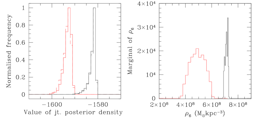
Figure 5: Left: figure showing histograms of the logarithm of the values of $\pi(\boldsymbol{\theta}_{B}|{\bf D}_{B})$ generated in two distinct 30,000 iteration-long, post-burnin parts of the chain run with synthetic data ${\bf D}_{B}$ (histograms of values of the posterior in the two distinct parts, are shown in solid and broken lines coloured grey–or red in the e-version). Similar histograms of values of $\pi(\boldsymbol{\theta}_{B}|{\bf D}_{B}^{(gen)})$ generated in two distinct 30,000 iterations-long, post-burnin parts of the chain run with generated data ${\bf D}_{B}^{(gen)}$, are shown in solid and broken, black lines. Right: figure showing the marginal posterior probability of the parameter $\rho_{6}$, given synthetic data ${\bf D}_{B}$, plotted in grey, (or in red in the electronic version) and the marginal of $\rho_{6}$ given and data ${\bf D}_{B}^{(gen)}$ (in black), where ${\bf D}_{B}^{(gen)}$ is sampled from the isotropic state space $pdf$ that is itself learnt using ${\bf D}_{B}$.

We corroborate convergence within the parts of the chains that we refer to as “post-burnin” in chains run with ${\bf D}_{B}$ and ${\bf D}_{B}^{(gen)}$ in Figure 5, by overplotting histograms of values of joint posterior probability density–of $\boldsymbol{\theta}_{B}$ given the data–generated over two distinct but equally long parts of such post-burnin stage of the chains. Concurrence of these generated histograms offers confidence in the convergence achieved in the post-burnin stage of the chains presented in the left panel of Figure 4. In Figure 5, we also present the marginal densities of the parameter $\rho_{6}$, given synthetic data ${\bf D}_{B}$ (sampled from a chosen state $pdf$ that is mildly anisotropic) and generated data ${\bf D}_{B}^{(gen)}$ (sampled from the isotropic $pdf$ that is learnt using data ${\bf D}_{B}$).

7 Testing for isotropic nature of state space of a real galaxy

In Section 2, we introduced the main application that we address in this work, namely that of learning the density function of all gravitating mass in the real galaxy NGC 3379, using two independent real data sets ${\bf D}_{1}$ observed by Bergond et al. (2006) and ${\bf D}_{2}$ observed by Douglas et al. (2007). These are two distinct data sets that bear information about 3–out of the 6–state space coordinates of two different kinds of galactic particles, referred to as planetary nebulae (PNe) and globular clusters (GCs). The data used in the work include measurements of $X_{1}$, $X_{2}$ and $V_{3}$ of 164 PNe reported by Douglas et al. (2007) and of 29 GCs by Bergond et al. (2006). From the estimate of (the discretised version $\boldsymbol{\rho}$ of) the gravitational mass density function of all types of matter in the galaxy, the mass density function of luminous matter in the galaxy can be subtracted, leaving us the mass density of the dark matter in the galaxy, which is a crucially important input into cosmological models. See Section 2 for details.

As the learning of $\boldsymbol{\rho}$ is possible only under the assumption that the available data is sampled from an isotropic state space density function, in this section, we discuss finding the probability of the null that the state space of this example real galaxy is isotropic, conditional on the measured data sets ${\bf D}_{1}$ and ${\bf D}_{2}$. Having estimated $\boldsymbol{\rho}$ using ${\bf D}_{1}$ and then using ${\bf D}_{2}$, each time assuming that the galactic state space is isotropic, we want to know in which case this assumption was more invalid, given the data. In other words, we want to find the comparative support for the null in these two data sets.

The physical implications of unequal supports for the assumption that the state space of a given galaxy is isotropic, can be most interesting–such would then imply that different sub-volumes of the galactic state space are differently anisotropic. This in turn implies that the state space of the galaxy is marked by at least two non-interacting sub-volumes, the dynamical structures of which are different, i.e. the distribution of the location $\boldsymbol{X}$ and velocity $\boldsymbol{V}$ vectors of the galactic particles in which are different. The non-linear dynamical implications of such difference is that the motions of particles in these sub-volumes do not communicate. Physical processes that cause such a split nature of the galactic state space will then be sought, and importantly, it will then be acknowledged that estimating the mass density of dark matter in a real galaxy using the available measurements on $X_{1},X_{2},V_{3}$ of one set of galactic particles–as is the usual practice in astrophysics–can be risky.

The null $H_{0}^{(i)}$, that data ${\bf D}_{i}$ is sampled from an isotropic state space density function $\Psi_{i}(E(X,V))$ is defined in Statement 3.1; $i=1,2$. Our new test, as described in Section 5, is implemented to estimate the conditional probability $\Pr(H_{0}|{\bf D}_{i})$ of the null $H_{0}^{(i)}$ given the data ${\bf D}_{i}$. To compute this, we generate data ${\bf D}_{i}^{(gen)}$ by rejection sampling from the discretised state space $pdf$ that is itself learnt using measured data ${\bf D}_{i}$) under the benchmark model ${\cal M}_{i}$ (in which $H_{0}^{(i)}$ is true).

To compute $\Pr(H_{0}|{\bf D}_{i})$, 3 chains: $i-RUN~{}I$, $i-RUN~{}II$ and $i-RUN~{}III$, that are distinguished by the seeds or initial guesses for the unknown parameters, are started with the available galactic data ${\bf D}_{i}$, for $i=1,2$, with the aim of learning the unknown model parameter vector $\boldsymbol{\theta}_{i}=(\Psi_{1}^{(i)},\ldots,\Psi_{N_{E}}^{(i)},\rho_{1}^{(i)},\ldots,\rho_{N_{x}}^{(i)})^{T}$, where the vector $\boldsymbol{\rho}_{i}=(\rho_{1}^{(i)},\ldots,\rho_{N_{x}}^{(i)})^{T}$ is the discretised version of the sought density function of gravitational mass of all matter in the galaxy and $\boldsymbol{\Psi}_{i}=(\Psi_{1}^{(i)},\ldots,\Psi_{N_{E}}^{(i)})^{T}$ is the discretised version of the state space density $\Psi_{i}(E)$, as learnt using the Bayesian scheme detailed in Section S-1 of the attached Supplementary Material, under the assumption that ${\bf D}_{i}$ is sampled from an isotropic state space density. The chains are at least 800,000 iterations long, and the unknown model parameter $\boldsymbol{\theta}_{i}$ is estimated using uniform priors on each scalar unknown, $\Psi_{j}^{(i)}$ and $\rho_{k}^{(i)}$, are used, $j=1,\ldots,N_{E}$, $k=1,\ldots,N_{x}$. From each chain, the identified ${\boldsymbol{\Psi}_{i}}^{(M,i)}$ at the identified $\boldsymbol{\rho}_{i}^{(M,i)}$ is used to generate a data set ${\bf D}_{i}^{(gen)}$ (see Section 5). A chain is run with this generated data set, in order to compute the minimal value of the posterior when the null is true. For each of the three chains initiated with different seeds and data ${\bf D}_{i}$, we identify the fractional number of samples of $\boldsymbol{\theta}_{i}$ for which $\pi(\boldsymbol{\theta}_{i}^{(min)}|{\bf D}_{i}^{(gen)})\leq\pi(\boldsymbol{\theta}_{i}|{\bf D}_{i})$, for each $i$=1,2. The results for each chain are presented in Table 3.

Table 3: Table showing support in data ${\bf D}_{i}$ for null $H_{0}^{(i)}$, $i=1,2$, computed using 3 different chains $i-RUN~{}j$ for each $i$; $i=1,2$, $j=I,II,III$.

Chain name	Data set used	$\Pr(H_{i}|{\bf D}_{i})$
$1-RUN~{}I$	${\bf D}_{1}$	0.6202
$1-RUN~{}II$	${\bf D}_{1}$	0.5862
$1-RUN~{}III$	${\bf D}_{1}$	0.6269
$2-RUN~{}I$	${\bf D}_{2}$	0.9617
$2-RUN~{}II$	${\bf D}_{2}$	0.9650
$2-RUN~{}III$	${\bf D}_{2}$	0.9348

Traces of the log of the posterior probabiliy density of $\boldsymbol{\theta}_{i}$ given real data ${\bf D}_{i}$ in the chains $i-RUN~{}I$, for $i=1,2$ are shown in Figure 6. The minimum value of the posterior density under the null $H_{0}^{(i)}$ is depicted in the solid line starting from the end of the burnin stage of the chain.

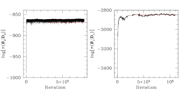
Figure 6: Trace of logarithm of the posterior probability density of the model parameter vector ${\boldsymbol{\theta}}_{1}$ (right panel) and $\boldsymbol{\theta}_{2}$ (left) given the two sets of real data ${\bf D}_{1}$ (size 164) and ${\bf D}_{2}$ (size 29) respectively, in chains $1-RUN~{}I$ and $2-RUN~{}I$. The minimal value of the posterior under the benchmark model (when the null is true given the corresponding generated data set), from the post-burnin stage of that chain (iteration 300,000 onwards), is shown in the solid grey (or red in the e-version) line.

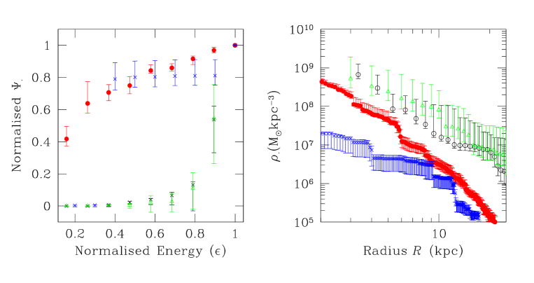
Figure 7: Right panel: logarithm of gravitational mass density vector $\boldsymbol{\rho}_{2}$ (in black, with modal values shown in open circles) learnt from chain $2-RUN~{}I$ that is run using data ${\bf D}_{2}$, and $\boldsymbol{\rho}_{1}$ from chain $1-RUN~{}I$ that is run using ${\bf D}_{1}$ (modal values shown in filled circles; in red in the e-version). These gravitational mass density results were obtained under the assumption of an isotropic state space, the support for which in the two data sets is indicated in Table 3. Overlaid on these are the identified vectors $\boldsymbol{\rho}_{1}^{(min)}$ (modal values in crosses; in blue in the e-version) and $\boldsymbol{\rho}_{2}^{(min)}$ (modal values in triangles; in green in the e-version), which are respectively, the posterior-minimising, null-abiding, gravitational mass density vectors identified in chains run with the generated data ${\bf D}_{1}^{(gen)}$ and ${\bf D}_{2}^{(gen)}$. The concurrence of $\boldsymbol{\rho}_{2}$ and $\boldsymbol{\rho}_{2}^{(min)}$ is noted, along with the lack of consistency between $\boldsymbol{\rho}_{1}$ and $\boldsymbol{\rho}_{1}^{(min)}$. The error bars represent the 95$\%$ HPD credible regions on the estimated $\rho_{\cdot}$ parameter. In the left panel, the state space density vectors ${\boldsymbol{\Psi}}_{1}$ (modal values in filled red circles) and ${\boldsymbol{\Psi}}_{2}$ (modal values in open black circles), learnt from the chains $1-RUN~{}I$ and $2-RUN~{}I$, are shown, compared respectively to ${\boldsymbol{\Psi}}_{1}^{(min)}$ (modal values in blue crosses) and ${\boldsymbol{\Psi}}_{2}^{(min)}$ (in green triangles). Again, the overlap of ${\boldsymbol{\Psi}}_{(2)}$ and ${\boldsymbol{\Psi}}_{2}{(min)}$ is noted, as is the discord between ${\boldsymbol{\Psi}}_{1}$ and ${\boldsymbol{\Psi}}_{1}^{(min)}$, especially at high and low energies. The ${\boldsymbol{\Psi}}$ vectors are normalised to unity at $\epsilon=1$ where $\epsilon$ is the value of the normalised energy.

Basically, support in real data ${\bf D}_{1}$ for the assumption of an isotropic state space, is distinct from that in ${\bf D}_{2}$. This implies that the $f_{1}({\boldsymbol{x},\boldsymbol{v}})\neq f_{2}({\boldsymbol{x},\boldsymbol{v}})$, where the true state space $pdf$ that ${\bf D}_{1}$ is sampled from is $f_{1}({\boldsymbol{x},\boldsymbol{v}})$ and ${\bf D}_{2}\sim f_{2}({\boldsymbol{x},\boldsymbol{v}})$. However, both data sets carry information on the state space coordinates $(X_{1},X_{2},X_{3},V_{1},V_{2},V_{3})^{T}$ in the same galactic state space, i.e. both data sets are sampled from $pdf$s that describe the state space structure of all or some volume inside the same galactic state space ${\cal W}$. Thus, $f_{1}({\boldsymbol{x},\boldsymbol{v}})\neq f_{2}({\boldsymbol{x},\boldsymbol{v}})\Longrightarrow{\cal W}_{1}\neq{\cal W}_{2}$ where $f_{1}({\boldsymbol{x},\boldsymbol{v}})$ is the $pdf$ of the state space vector that lives in volume ${\cal W}_{1}\subset{\cal W}$ and $f_{2}({\boldsymbol{x},\boldsymbol{v}})$ is the density of the state space vector in volume ${\cal W}_{2}\subset{\cal W}$. In terms of the state space structure of this real galaxy NGC 3379, we can then conclude that the state space of the system is marked by at least two distinct volumes, motions in which do not communicate with each other, leading to distinct particle distributions being set up in these two volumes, which in turn manifests in distinct $pdf$s for these subspaces (${\cal W}_{1}$ and ${\cal W}_{2}$) of the galactic state space ${\cal W}$. Data ${\bf D}_{1}$ and ${\bf D}_{2}$ are respectively drawn from such distinct $pdf$s.

Comparing the computed $\Pr(H_{0}^{(1)}|{\bf D}_{1})$ and $\Pr(H_{0}^{(2)}|{\bf D}_{2})$, we can see that the assumption of isotropy is more likely to be invalid for the state space density from which the data ${\bf D}_{1}$ are sampled than from which the data ${\bf D}_{2}$ are drawn. Even beyond comparative terms, our results indicate that $\Pr(H_{0}^{(2)}|{\bf D}_{2})\approx 1$, i.e. we reject the isotropy of the state space density that the observed data ${\bf D}_{2}$ in this galaxy live in at nearly 0 probability.

8 Discussions

In the above test, a high support in ${\bf D}_{2}$ towards an isotropic state space $pdf$, along with a moderate support in ${\bf D}_{1}$ for the same assumption, indicate that the two samples are drawn from two distinct state space densities.

Any apriori expectation that the implementation of the PNe and GC data sets will lead to concurring gravitational mass density estimates is foreshadowed by the assumption that both data sets are sampled from the same - namely, the galactic - state space density $f(\boldsymbol{X},\boldsymbol{V})$. Such an expectation can be understood to emanate from the argument that since both samples live in the galactic phase space ${\cal W}$, they are expected to be sampled from the same galactic state space density, at the galactic gravitational potential. However, such does not necessarily follow if–for example–the galactic state space density $f({\boldsymbol{X},\boldsymbol{V}})$ is a non-analytic function with $p_{max}$ branches:

$$f({\boldsymbol{X},\boldsymbol{V}})=f_{p}({\boldsymbol{X},\boldsymbol{V}}),\quad\forall{(X_{1},X_{2},X_{3},V_{1},V_{2},V_{3})^{T}}\in{\cal W}_{p}\subseteq{\cal W},\quad p=1,\ldots,p_{max}.$$ (8.1)

Then, if the data ${\bf D}_{2}$ are sampled from the density $f_{2}(\cdot)$ and data ${\bf D}_{1}\sim f_{1}(\cdot)$, it follows that ${\bf D}_{1}$ and ${\bf D}_{2}$ are sampled from unequal state space densities. Qualitatively we understand that if the galactic state space ${\cal W}$ is split into isolated volumes, such that the motions in these volumes do not mix and are therefore distinctly distributed in general, the state space densities of these volumes would be unequal. This is synonymous to saying that ${\cal W}$ is marked by at least two distinct basins of attraction and the two observed samples reside in such distinct basins.

One standard non-linear dynamical cause for the splitting of ${\cal W}$ include the development of basins of attraction, leading to attractors, generated in a multistable galactic gravitational potential. Basins of attraction could also be triggered around chaotic attractors, which in turn could be due to resonance interaction with external perturbers or due to merging events in the evolutionary history of the galaxy. Galactic state spaces can be split given that a galaxy is expectedly a complex system, built of multiple components with independent evolutionary histories and distinct dynamical timescales. As an example, at least in the neighbourhood of the Sun, the state space structure of the Milky Way is highly multi-modal and the ensuing dynamics is highly non-linear, marked by significant chaoticity.

Supplementary material

Details of the Bayesian learning of the gravitational mass density and state space $pdf$ of the galaxy are provided in Section S-1 of the attached supplementary material. Section S-2 discusses details of the Fully Bayesian Significance Test.

References

- (1)
- Aitkin (1991) Aitkin, M. (1991), “Posterior Bayes factors,” Journal of the Royal Statistical Society Series B, 53, 111–142.
- Barbieri and Berger (2004) Barbieri, M., and Berger, J. (2004), “Optimal predictive model selection,” The Annals of Statistics, 32, 870–897.
- Bell and de Jong (2001) Bell, E. F., and de Jong, R. S. (2001), “Stellar Mass-to-Light Ratios and the Tully-Fisher Relation,” Astrophysical Journal, 550(1), 212.
- Berger and Pericchi (2001) Berger, J. O., and Pericchi, L. R. (2001), “Objective Bayesian Methods for Model Selection: Introduction and Comparison,” in Model Selection, ed. P. Lahiri, Vol. 38 of Lecture Notes–Monograph Series, Beachwood, OH: Institute of Mathematical Statistics, pp. 135–207.
- Berger and Pericchi (1996a) Berger, J., and Pericchi, L. (1996a), “The intrinsic Bayes factor for model selection and prediction,” Journal of the American Statistical Association, 57, 109–122.
- Berger and Pericchi (1996b) Berger, J., and Pericchi, L. (1996b), “The intrinsic Bayes factor for linear models,” in Bayesian Statistics, 5, eds. J. M. Bernardo, J. O. Berger, A. P. Dawid, and A. F. M. Smith Oxford University Press, pp. 25–44.
- Berger and Pericchi (2004) Berger, J., and Pericchi, L. (2004), “Training samples in objective Bayesian model selection,” The Annals of Statistics, 32, 841–869.
- Bergond et al. (2006) Bergond, G., Zepf, S. E., Romanowsky, A. J., Sharples, R. M., and Rhode, K. L. (2006), “Wide-field kinematics of globular clusters in the Leo I group,” Astronomy Astrophysics, 448, 155–164.
- Casella et al. (2009) Casella, G., Girón, F. J., Martínez, M. L., and Moreno, E. (2009), “Consistency of Bayesian procedures for variable selection,” Annals of Statistics, 37, 3, 1207–1228.
- Chakrabarty and Raychaudhury (2008) Chakrabarty, D., and Raychaudhury, S. (2008), “The Distribution of Dark Matter in the Halo of the Early-Type Galaxy NGC 4636,” Astronomical Journal, 135, 2350–2357.
- Chib and Jeliazkov (2001) Chib, S., and Jeliazkov, I. (2001), “Marginal likelihood from the Metropolis-Hastings output,” Journal of the American Statistical Association, 96, 453, 270–281.
- Chipman et al. (2001) Chipman, H., George, E., and McCulloch, R. E. (2001), “The practical implementation of Bayesian model selection (with discussion),” in Model Selection, IMS Lecture Series - Monograph Series, ed. P. Lahiri, Vol. 38 Beachwood, OH: Institute of Mathematical Statistics, pp. 67–134.
- Coccato et al. (2009) Coccato, L., Gerhard, ., Arnaboldi, M., and et al. (2009), “Kinematic properties of early-type galaxy haloes using planetary nebulae,” Monthly Notices of the Royal Astronomical Society, 394, 1249.
- Côté et al. (2001) Côté, P., McLaughlin, D. E., Hanes, D. A., Bridges, T. J., Geislerand D. Merritt, D., Hesser, J. E., Harris, G. L. H., and Lee, M. G. (2001), “Dynamics of the Globular Cluster System Associated with M87 (NGC 4486). II. Analysis,” Astrophysical Jl., 559, 828–850.
- Dalal et al. (1989) Dalal, S. R., Fowlkes, E. B., and Hoadley, B. (1989), “Risk analysis of the space shuttle: Pre-Challenger prediction of failure,” Journal of the American Statistical Association, 84, 945–957.
- de Blok et al. (2003) de Blok, W. J. G., Bosma, A., and McGaugh, S. (2003), “Simulating observations of dark matter dominated galaxies: towards the optimal halo profile,” Monthly Notices of the Royal Astronomical Soc, 340, 657–678.
- Dekel et al. (2005) Dekel, A., Stoehr, F., Mamon, G. A., Cox, T. J., Novak, G. S., and Primack, J. R. (2005), “Lost and found dark matter in elliptical galaxies,” Nature, 437, 707–710.
- Douglas et al. (2007) Douglas, N. G., Napolitano, N. R., Romanowsky, A. J., Coccato, L., Kuijken, K., Merrifield, M. R., Arnaboldi, M., Gerhard, O., Freeman, K. C., Merrett, H., Noordermeer, E., and Capaccioli, M. (2007), “The PN.S Elliptical Galaxy Survey: Data Reduction, Planetary Nebula Catalog, and Basic Dynamics for NGC 3379,” Astrophysical Jl., 664, 257–276.
- Fouskakis et al. (2015) Fouskakis, D., Ntzoufrasy, I., and Draper, D. (2015), “Power-Expected-Posterior Priors for Variable Selection in Gaussian Linear Models,” Bayesian Analysis, 10(1), 75–107.
- Gallazzi and Bell (2009) Gallazzi, A., and Bell, E. F. (2009), “Stellar Mass-to-Light Ratios from Galaxy Spectra: How Accurate Can They Be?,” Astrophysical Jl. Supplement, 185, 253–272.
- Genzel et al. (2003) Genzel, R., Schödel, R., Ott, T., Eisenhauer, F., Hofmann, R., Lehnert, M., Eckart, A., Alexander, T., Sternberg, A., Lenzen, R., Clénet, Y., Lacombe, F., Rouan, D., Renzini, A., and Tacconi-Garman, L. E. (2003), “The Stellar Cusp around the Supermassive Black Hole in the Galactic Center,” Astrophysical Jl., 594, 812–832.
- Ghosh and Samanta (2001) Ghosh, J. K., and Samanta, T. (2001), “Model selection - An overview,” Current Statistics, 80, 1135–1144.
- Han and Carlin (2000) Han, C., and Carlin, B. P. (2000), “MCMC Methods for Computing Bayes Factors: A Comparative Review,” Journal of the American Statistical Association, 96, 1122–1132.
- Hayashi et al. (2007) Hayashi, E., Navarro, J. F., and Springel, V. (2007), “The shape of the gravitational potential in cold dark matter haloes,” Monthly Notices of the Royal Astronomical Society, 377, 50–62.
- Kalinova (2014) Kalinova, V. (2014), Mass Distributions of Galaxies from SAURON and CALIFA Stellar Kinematic Maps, Doctoral thesis, Max-Planck-Institut f¨ur Astronomie.
- Kass and Raftery (1995) Kass, R. E., and Raftery, A. E. (1995), “Bayes Factors,” JASA, 90(430), 773–795.
- Leone et al. (1961) Leone, F., Nottingham, R. B., and Nelson, L. S. (1961), “The Folded Normal Distribution,” Technometrics, 3(4), 543.
- Link and Barker (2006) Link, W. A., and Barker, R. J. (2006), “Model weights and the foundations of multimodal inference,” Ecology, 87, 2626–2635.
- Liu (2002) Liu, I.-S. (2002), Continuum Mechanics, New York: Springer-Verlag.
- Madruga et al. (2003) Madruga, M., Pereira, C., and Stern, J. (2003), “Bayesian evidence test for precise hypotheses,” Journal of Statistical Planning and Inference, 117, 185–198.
- Neal (1998) Neal, R. M. (1998), “Regression and classification using Gaussian process priors (with discussion),” in Bayesian Statistics 6, ed. J. M. B. et. al Oxford University Press, pp. 475–501.
- O’Hagan (1995) O’Hagan, A. (1995), “Fractional Bayes Factors for Model Comparisons,” Journal of Royal Statistical Society, Ser. B, 57, 99–138.
- Pereira et al. (2008) Pereira, C., J.M.Stern, and S.Wechsler (2008), “Can a Significance Test be Genuinely Bayesian?,” Bayesian Analysis, 3(1), 79–100.
- Pierce and et al. (2006) Pierce, M., and et al. (2006), “Gemini/GMOS spectra of globular clusters in the Leo group elliptical NGC 3379,” Monthly Notices of the Royal Astronomical Society, 366, 1253.
- Robert (2001) Robert, C. (2001), The Bayesian Choice, New York: Springer.
- Robert and Casella (2004) Robert, C. P., and Casella, G. (2004), Monte Carlo Statistical Methods, New York: Springer-Verlag.
- Roberts and Whitehurst (1975) Roberts, M. S., and Whitehurst, R. N. (1975), “The rotation curve and geometry of M31 at large galactocentric distances.,” Astrophysical Jl., 201, 327–346.
- Romanowsky et al. (2003) Romanowsky, A. J., Douglas, N. G., Arnaboldi, M., Kuijken, K., Merrifield, M. R., Napolitano, N. R., Capaccioli, M., and Freeman, K. C. (2003), “A Dearth of Dark Matter in Ordinary Elliptical Galaxies,” Science, 301, 1696–1698.
- Salucci and Burkert (2000) Salucci, P., and Burkert, A. (2000), “Dark Matter Scaling Relations,” Astrophysical Jl. Letters, 537, L9–L12.
- Sofue and Rubin (2001) Sofue, Y., and Rubin, V. (2001), “Rotation Curves of Spiral Galaxies,” Annual Review of Astronomy Astrophysics, 39, 137–174.
- Truesdell et al. (2004) Truesdell, C., Noll, W., and Antman, S. S. (2004), The non-linear field theories of mechanics, number Volume 3, New York: Springer-Verlag.
- Wang (1969) Wang, C. C. (1969), “On representations for isotropic functions,” Archive for Rational Mechanics and Analysis, 33, 249–267.
- Weijmans and et al. (2009) Weijmans, A. M., and et al. (2009), “Stellar velocity profiles and line strengths out to four effective radii in the early-type galaxies NGC 3379 and NGC 821,” Monthly Notices of the Royal Astronomical Society, 398, 561.