A Competitive Strategy for
Distance-Aware Online Shape Allocation

Abstract

We consider the following online allocation problem: Given a unit square $S$, and a sequence of numbers $n_{i}\in\{0,1\}$ with $\sum_{j=0}^{i}n_{j}\leq 1$; at each step $i$, select a region $C_{i}$ of previously unassigned area $n_{i}$ in $S$. The objective is to make these regions compact in a distance-aware sense: minimize the maximum (normalized) average Manhattan distance between points from the same set $C_{i}$. Related location problems have received a considerable amount of attention; in particular, the problem of determining the “optimal shape of a city”, i.e., allocating a single $n_{i}$ has been studied. We present an online strategy, based on an analysis of space-filling curves; for continuous shapes, we prove a factor of 1.8092, and 1.7848 for discrete point sets.

1 Introduction

Many optimization problems deal with allocating point sets to a given environment. Frequently, the problem is to find compact allocations, placing points from the same set closely together. One well-established measure is the average $L_{1}$ distance between points. A practical example occurs in the context of grid computing, where one needs to assign a sequence of jobs $i$, each requiring an (appropriately normalized) number $n_{i}$ of processors, to a subset $C_{i}$ of nodes of a large square grid, such that the average communication delay between nodes of the same job is minimized; this delay corresponds to the number of grid hops leung , so the task amounts to finding subsets with a small average $L_{1}$, i.e., Manhattan distance. Karp et al. karp studied the same problem in the context of memory allocation.

Even in an offline setting without occupied nodes, finding an optimal allocation for one set of size $n_{i}$ is not an easy task; as shown in Fig. 1, the results are typically “round” shapes. If a whole sequence of sets have to be allocated, packing such shapes onto the grid will produce gaps, causing later sets to become disconnected, and thus leads to extremely bad average distances. Even restricting the shapes to be rectangular is not a remedy, as the resulting problem of deciding whether a set of squares (which are minimal with respect to $L_{1}$ average distance among all rectangles) can be packed into a given square container is NP-hard squaresquare ; moreover, disconnected allocations may still occur.

In this paper, we give a first algorithmic analysis for the online problem. Using an allocation scheme based on a space-filling curve, we establish competitive factors of 1.8092 and 1.7848 for minimizing the maximum average Manhattan distance within an allocated set.

Related Work

Compact location problems have received a considerable amount of attention. Krumke et al. krumke have considered the offline problem of choosing a set of $n$ vertices in a weighted graph, such that the average distance is minimized. They showed that the problem is NP-hard (even to approximate); for the scenario in which distances satisfy the triangle inequality, they gave algorithms that achieve asymptotic approximation factors of 2. For points in two-dimensional space and Manhattan distances, Bender et al. bender2 gave a simple 1.75-approximation algorithm, and a polynomial-time approximation scheme for any fixed dimension.

The problem of finding the “optimal shape of a city”, i.e., a shape of given area that minimizes the average Manhattan distance, was first considered by Karp, McKellar, and Wong karp ; independently, Bender, Bender, Demaine, and Fekete bender showed that this shape can be characterized by a differential equation for which no closed form is known. For the case of a finite set of $n$ points that needs to be allocated to a grid, Demaine et al. dfr-psmd-11 showed that there is an $O(n^{7.5})$ dynamic-programming algorithm, which allowed them to compute all optimal shapes up to $n=80$. Note that all these results are strictly offline, even though the original motivation (register or processor allocation) is online.

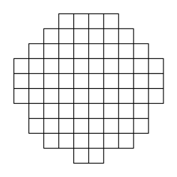
Figure 1: Finding optimal individual shapes. (Left) An optimal shape composed of n=72 grid cells, according to dfr-psmd-11 . (Right) The optimal limit curve $w(x)$, according to bender2 .

Space-filling curves for processor allocation with our objective function have been used before, see Leung et al. leung ; however, no algorithmic results and no competitive factor was proven. Wattenberg w-nsfvs-05 proposed an allocation scheme similar to ours, for purposes of minimizing the maximum Euclidean diameter of an allocated shape. Like other authors before (in particular, Niedermeier et al. nrs-tolmi-02 and Gotsman and Lindenbaum gl-mpdsf-96 ), he considered a measure called $c$-locality: for a sequence $1,\ldots,i,\ldots,j,\ldots$ of points on a line, a space-filling mapping $h(.)$ will guarantee $L_{2}(h(i),h(j))<c\sqrt{|j-i|}$, for a constant $c$ that is $\sqrt{6}\approx 2.449$ for the Hilbert curve, and 2 for the so-called H-curve. One can use $c$-locality for establishing a constant competitive factor for our problems; however, given that the focus is on bounding the worst-case distance ratio for an embedding instead of the average distance, it should come as no surprise that the resulting values are significantly worse than the ones we achieve. On a different note, de Berg, Speckmann, and van der Weele  DBLP:journals/corr/abs-1012-1749 consider treemaps with bounded aspect ratio. Other related work includes Dai and Su ds-lpsfc-03 .

Our Results

We give a first competitive analysis for the online shape allocation problem within a given bounding box, with the objective of minimizing the maximum average Manhattan distance. In particular, we give the following results.

• We show that for the case of continuous shapes (in which numbers $n_{i}$ correspond to area), a strategy based on a space-filling Hilbert curve achieves a competitive ratio of 1.8092.

• For the case of discrete point sets (in which numbers indicate the number of points that have to be chosen from an appropriate $N\times N$ orthogonal grid), we prove a competitive factor of 1.7848.

• We sketch how these factors may be further improved, but point out that a Hilbert-based strategy is no better than a competitive factor of 1.3504, even with an improved analysis.

• We establish a lower bound of 1.144866 for any online strategy in the case of discrete point sets, and argue the existence of a lower bound for the continuous case.

The rest of this paper is organized as follows. In Section 2, we give some basic definitions and fundamental facts. In Section 3, we provide a brief description of an allocation scheme based on a space-filling curve. Section 4 gives a mathematical study for the case of continuous allocations, proving that the analysis can be reduced to a limited number of shapes, and establishes a competitive factor of 1.8092. Section 5 sketches a similar analysis for the case of discrete allocations; as a result, we prove a competitive factor of 1.7848. Section 6 discusses lower bounds for online strategies. Final conclusions are presented in Section 7.

2 Preliminaries

We examine the problem of selecting shapes from a square, such that the maximum average $L_{1}$-distance of the shapes is minimized. We first formulate the problem more precisely. This covers both the continuous and the discrete case; the former arises as the limiting case of the latter, while the latter needs to be considered for allocations within a grid of limited size.

Definition 1

A city is a (continuous) shape in the plane with fixed area. For a city $C$ of area $n$, we call

$$c(C)=\frac{1}{2}\iiiint_{(x,y),(u,v)\in C}(|x-u|+|y-v|)\,\mathrm{d}v\,\mathrm{d}u\,\mathrm{d}y\,\mathrm{d}x$$ (1)

the total Manhattan distance between all pairs of points in $C$ and

$$\phi(C)=\frac{2\,c(C)}{n^{5/2}}$$ (2)

the $\phi$-value or average distance of $C$. An $n$-town $T$ is a subset of $n$ points in the integer grid. Its normalized average Manhattan distance is

$$\phi(T)=\frac{2c(T)}{n^{5/2}}=\frac{\sum_{s\in T}\sum_{t\in T}\|s-t\|_{1}}{n^{5/2}}$$ (3)

The normalization with $n^{2.5}$ yields a dimensionless measure that remains unchanged under scaling, and makes the continuous and the discrete case comparable; see bender .

Problem 2

In the continuous setting, we are given a sequence $n_{1},n_{2},\ldots,n_{k}\in\mathbb{R}^{+}$ with $\sum_{i=1}^{k}{n_{i}}\leq 1$. Cities $C_{1},C_{2},\ldots,C_{k}$ of size $n_{1},n_{2},\ldots,n_{k}$ are to be chosen from the unit square, such that $\max_{1\leq i\leq k}{\phi(C_{i})}$ is minimized.

In the discrete setting, we are given a sequence $n_{1},n_{2},\ldots,n_{k}\in\mathbb{N}^{+}$ with $\sum_{i=1}^{k}{n_{i}}\leq N^{2}$. Towns $C_{1},C_{2},\ldots,C_{k}$ of size $n_{1},n_{2},\ldots,n_{k}$ are to be chosen from the $N\times N$ grid, such that $\max_{1\leq i\leq k}{\phi(C_{i})}$ is minimized.

Although it has not been formally proven, the offline problem is conjectured to be NP-hard, see schweer ; if we restrict city shapes to be rectangles, there is an immediate reduction from deciding whether a set of squares can be packed into a larger square squaresquare . (A special case arises from considering integers, which corresponds to choosing grid locations.) Our approximation works online, i.e., we choose the cities in a specified order, and no changes can be made to previously allocated cities; clearly, this implies approximation factors for the corresponding offline problems.

There are lower bounds for $\max_{1\leq i\leq k}\phi(C_{i})$ that generally cannot be achieved by any algorithm. One important result is the following theorem.

Theorem 3

Let $C$ be any city. Then $\phi(C)\geq 0.650245$.

A proof can be found in bender . For $n_{1}=1$ any algorithm must select the whole unit square, thus $2/3$, the $\phi$-value of a square, is a lower bound for the achievable $\phi$-value. We will discuss better lower bounds in the conclusions.

3 An Allocation Strategy

While long and narrow shapes tend to have large $\phi$-values, shapes that fill large parts of an enclosing rectangle with similar width and height usually have better average distances; however, one has to make sure that early choices with small average distance do not leave narrow pieces with high average distance, or even disconnected pieces, making the normalized $\phi$-values potentially unbounded.

Our approach uses the recursive Hilbert family of curves in order to yield a provably constant competitive factor. That family is based on a recursive construction scheme and becomes space-filling for infinite repetition of said scheme sagan . For a finite number $r$ of repetitions, the curve traverses all points of the used grid. For $1\leq r\leq 3$, the curve is shown in Fig. 2. Thus, the Hilbert curve provides an order for the cells of the grid, which is then used for allocation, as illustrated in Fig. 3. More formal details of the recursive definition of the Hilbert family (e.g. with text-rewriting rules, such as the ones in hilb-grammar ) are cited and sketched in the following Section 4.

Figure 2: Hilbert curve with $1\leq r\leq 3$.

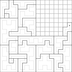
Figure 3: A sample allocation according to our strategy.

More technically, the unit square is recursively subdivided into a grid consisting of $2^{r}\times 2^{r}$ grid cells, for an appropriate refinement level $r>0$, as shown in Fig. 2. For the sake of concise presentation, we assume that every input $n_{i}$ is an integral multiple of $c=4^{-R}$, for an appropriately large $R>0$. (We will mention in the Conclusions how this assumption can be removed, based on Lemma 10.) Similar to the recursive structure of quad-trees, the actual subdivision can be performed in a self-refining manner, whenever a grid cell is not completely filled. This means that during the course of the online allocation, we may use different refinement levels in different parts of the layout; however, this will not affect the overall analysis, as further refinement of the grid does not change the quality of existing shapes.

Definition 4

For a give refinement level $r$, an $r$-pixel $P$ is a grid square of size $2^{-r}\times 2^{-r}$. For a given allocated shape $C_{i}$, a pixel is full if $P\subseteq C_{i}$; it is fractional, if $P\cap C_{i}\neq\emptyset$ and $P\not\subset C_{i}$.

Now the description of the algorithm is simple: for every input $n_{i}$, choose the next set of $n_{i}/2^{R}$ $R$-pixels traversed by the Hilbert curve as the city $C_{i}$, starting in the upper left corner of the grid. For an illustration, see Fig. 3.

The following lemma is a consequence of the recursive structure of the Hilbert family; see the following Section 4 for a formal argument. We use it in Section 5 for deriving upper bounds.

Lemma 5

Let $C$ be a city generated by our strategy with area at most $n\leq l\,4^{j}\,4^{-R}$ for $j\in\{0,1,\ldots,R\},l\in\mathbb{N}$. Then at any refinement level $r$, $C$ contains at most two fractional $r$-pixels.

4 Technical Details of Shape Allocation

A technical different description of the Hilbert family can be based on the string representation given in hilb-grammar . There, the authors use the following recursion, based on the letters u, r, d, l for denoting “up”, “right”, “down”, and “left”.

$$y_{1} = \mathrm{urd}$$

$$y_{n} = h_{4}(y_{n-1})\mathrm{u}y_{n-1}\mathrm{r}y_{n-1}\mathrm{d}h_{5}(y_{n-1})\mathrm{\mbox{ if }}n>1$$

where $h_{4}$ and $h_{5}$ are defined as

$$h_{4}(x)=\begin{cases}\text{r}&\text{if }x=\text{u},\\ \text{l}&\text{if }x=\text{d},\\ \text{u}&\text{if }x=\text{r},\\ \text{d}&\text{if }x=\text{l}.\end{cases}\mathrm{\mbox{ and }}h_{5}(x)=\begin{cases}\text{l}&\text{if }x=\text{u},\\ \text{r}&\text{if }x=\text{d},\\ \text{d}&\text{if }x=\text{r},\\ \text{u}&\text{if }x=\text{l}.\end{cases}$$

and $h_{i}(x_{0}x_{1}x_{2}\ldots)=h_{i}(x_{0})h_{i}(x_{1})h_{i}(x_{2})\ldots$, $i\in\{4,5\}$.

We combine those characters to four sequences of length three and build an L-system, a special kind of formal grammar with parallel rewriting. Let $A=\mathrm{urd}$, $B=\mathrm{ldr}$, $C=\mathrm{rul}$, and $D=\mathrm{dlu}$, as shown in Figure 4 Using the production rules

$$A \rightarrow CAAB,$$

$$B \rightarrow DBBA,$$

$$C \rightarrow ACCD\mathrm{\mbox{ and }}$$

$$D \rightarrow BDDC$$

and starting with $A$, you get the same string from hilb-grammar if you replace $X_{0}X_{1}X_{2}X_{3}$ by $X_{0}uX_{1}rX_{2}dX_{3}$, $X_{0},X_{1},X_{2},X_{3}\in\{A,B,C,D\}$, after each use of a production rule.

A sequence of symbols produced by the L-system can be interpreted graphically as a sequence of sub-squares $E_{r-1}^{2}[j][k],j,k\in\{1,\ldots,2^{r-1}\}$, see Figure 4. The figure also shows that $A$ is $D$ rotated by $180^{\circ}$. The same is true for $B$ and $C$. We denote by $\overline{X}$ the symbol that is $X$ rotated by $180^{\circ}$. As we are only interested in the shape of cities, we identify symmetric cities. Consequently, we make no distinction between $X$ and $\overline{X}$ when we look at a single symbol. We write $X\equiv\overline{X}$. Similarly, we get equivalences for longer sequences of symbols: $XY\equiv YX$, because the order of the successive sub-squares $E_{r-1}^{2}[j][k]$ does not change the shape. Furthermore, we have $X\overline{X}\equiv Y\overline{Y}$ for each $X$ and $Y$, as it is always the simple shape followed by the rotated shape, and $XX\equiv\overline{X}\overline{X}$ for two occurrences of the same shape in succession.

Figure 4: $A$, $B$, $C$, and $D$

Lemma 6

After $r>1$ uses of the production rules (where $r=1$ means that we are still at the start symbol $A$), the resulting sequence contains all sub-sequences of length $2^{r-2}$ that can be created with the L-system, except for symmetry.

Proof: We prove the claim via induction over $r$:

$r=2:$

$CAAB$ contains $C$, $B$, and $A\equiv\overline{A}=D$, i.e., all sequences of length 1.

$r=3:$

$ACCDCAABCAABDBBA$ contains

• $AA\equiv DD$

• $AB\equiv BA\equiv DC\equiv CD$

• $AC\equiv CA\equiv DB\equiv BD$

• $BC\equiv CB\equiv AD\equiv DA$

• $BB\equiv CC$,

i.e, all possible sequences of length 2.

$r\rightarrow r+1,r\geq 3:$

A sequence of length $2^{r-1}$ has been created from a sequence of length at most $2^{r-1}/4+1=2^{r-3}+1$, because every symbol is replaced by exactly 4 symbols. If the claim holds for $r\geq 3$, then all sequences of length $2^{r-2}$ have been created, i.e., all sequences of length $2^{r-3}+1$ have been created as well. Thus, in the next step the production rules are applied to all possible sequences of that length, yielding all sequences of length $2^{r-1}$ that can be created with the L-system.

$\Box$

Lemma 7

A city $W_{n}$ contains at most parts of $\lceil n/4\rceil+1$ sub-squares $E_{r-1}^{2}[j][k]$, $j,k\in\{1,\ldots,2^{r-1}\}$, i.e., sub-squares that consist of exactly 4 cells.

Proof: A city $W_{n}$ consists of exactly $n$ cells. Assume that these cells belong to at least $\lceil n/4\rceil+2$ sub-squares $E_{r-1}^{2}[j][k]$. Then at least three of those sub-squares cannot belong to $W_{n}$ as a whole but only in part, because $n$ cells cannot completely fill more than $\lceil n/4\rceil$ of the sub-squares, and if two more are partially filled not even all those can be filled completely. Consider the sequence of sub-squares of $W_{n}$ in the order given by the Hilbert curve. One of the sub-squares that is not the first or the last in the sequence cannot completely belong to $W_{n}$. This is a contradiction to the definition of the Hilbert curve, which recursively uses the same construction scheme for sub-squares on every level of refinement.

Lemma 8

When the L-system has generated all sequences of length $\lceil n/4\rceil+1$, the resulting Hilbert curve traverses a city $W_{n}$.

Proof: Each symbol of the L-system corresponds to a sub-square $E_{r-1}^{2}[j][k]$. Once all sequences of length $\lceil n/4\rceil+1$ symbols have been generated, all possible cities consisting of $\lceil n/4\rceil+1$ sub-squares have been generated, too. With Lemma 7 the claim follows.

Lemma 9

For $r=\lceil\log_{2}(\lceil n/4\rceil+1)\rceil+2$ the Hilbert curve traverses a city $W_{n}$.

Proof: Using Lemmas 6 and 8 we know that the Hilbert curve traverses a city $W_{n}$, if the following holds:

$$2^{r-2}\geq\lceil n/4\rceil+1$$

This is true for

$$r=\lceil\log_{2}(\lceil n/4\rceil+1)\rceil+2.$$

5 Analysis

For the analysis of our allocation scheme we will first make use of Lemma 5. As noted in Lemma 10, filling in the two fractional pixels of an allocated shape yields an estimate for the total distance at a coarser refinement level. In a second step, this will be used to derive global bounds by computing the worst-case bounds for shapes of at most refinement level 3; thus the presented computational results for shapes of limited size are not merely experiments, but yield a general upper bound on the competitive factor. (As discussed in the Conclusions, carrying out the computations on a lower or higher refinement level gives looser or tighter results.)

In the following, we denote by $W_{n}$ the worst city consisting of $n$ pixels that can be produced by our Hilbert strategy; because of the normalized nature of $\phi$, this is independent on the size of the pixels, and only the shape matters.

Lemma 10

Let $C$ be a city generated by our strategy with area at most $n\leq l\,4^{r}\,4^{-R}$ for $r\in\{0,1,\ldots,R\},l\in\mathbb{N}$. Then we have $c(C)\leq c(W_{l+1})$, where $W_{l+1}$ is a worst case among all cities produced by our allocation scheme that consists of $(l+1)$ $r$-pixels.

Proof: By Lemma 5, we know that only the first and the last pixel of $C$ may be fractional. Therefore $C$ cannot intersect more than $l+1$ $r$-pixels. By replacing the two fractional pixels by full pixels, we get a city $W$ that consists of $l+1$ full $r$-pixels, and $c(C)\leq c(W)$. By definition, $c(W)\leq c(W_{l+1})$, and the claim holds.

Therefore, we can give upper bounds for the worst case by considering the values of $W_{n}$ at some moderate refinement level. The $W_{n}$ can be found by enumeration; as described by the technical lemmas in preceding section, a speed-up can be achieved by making use of the recursive construction of the $W_{n}$. We determined the shapes and $\phi$-values of the $W_{n}$ for $n\leq 65$; by Lemma 10, this suffices to provide upper bounds for all cities with area up to $64*2^{-r}$, i.e., these computational results give an estimate for the round-up error using refinement level 3. The full table of average distances for this refinement level can be seen in Table 1; the worst cases among the examined ones are $W_{56}$ and $W_{14}$, which have the same shape, shown in Fig. 5.

Figure 5: Worst cases $W_{n}$ for $12\leq n\leq 17$.

Table 1: Total and average distances for cities $W_{n}$ allocated according to our strategy, as well as the optimal values $c_{city}(n)$ according to dfr-psmd-11 .

$n$	$c^{*}(W_{n})$	$c_{{city}}(n)$	$\phi(W_{n})$	$\Phi(W_{n})$	$n$	$c^{*}(W_{n})$	$c_{{city}}(n)$	$\phi(W_{n})$	$\Phi(W_{n})$
$1$	$0\,^{1}/_{3}$	$0\,^{1}/_{3}$	$0.6667$		$34$	$2835\,^{2}/_{3}$	$2216\,^{2}/_{3}$	$0.8414$	$0.9691$
$2$	$2$	$2$	$0.7071$		$35$	$3045$	$2384$	$0.8403$	$0.9712$
$3$	$6$	$5\,^{2}/_{3}$	$0.7698$		$36$	$3266$	$2554\,^{2}/_{3}$	$0.8400$	$0.9772$
$4$	$13\,^{1}/_{3}$	$10\,^{2}/_{3}$	$0.8333$		$37$	$3519\,^{1}/_{3}$	$2727\,^{2}/_{3}$	$0.8453$	$0.9726$
$5$	$24$	$19\,^{2}/_{3}$	$0.8587$		$38$	$3799\,^{1}/_{3}$	$2921\,^{2}/_{3}$	$0.8536$	$0.9682$
$6$	$38$	$30$	$0.8619$		$39$	$4049\,^{2}/_{3}$	$3117\,^{2}/_{3}$	$0.8527$	$0.9570$
$7$	$50\,^{2}/_{3}$	$44$	$0.7816$		$40$	$4309\,^{1}/_{3}$	$3322$	$0.8517$	$0.9463$
$8$	$74\,^{2}/_{3}$	$61\,^{1}/_{3}$	$0.8250$		$41$	$4545$	$3530\,^{1}/_{3}$	$0.8445$	$0.9307$
$9$	$102$	$81$	$0.8395$		$42$	$4788$	$3749$	$0.8376$	$0.9214$
$10$	$134\,^{2}/_{3}$	$106\,^{1}/_{3}$	$0.8517$		$43$	$5009$	$3976$	$0.8262$	$0.9306$
$11$	$162$	$135\,^{2}/_{3}$	$0.8074$		$44$	$5266\,^{2}/_{3}$	$4205\,^{1}/_{3}$	$0.8202$	$0.9393$
$12$	$210\,^{2}/_{3}$	$165\,^{1}/_{3}$	$0.8446$		$45$	$5641\,^{1}/_{3}$	$4456\,^{2}/_{3}$	$0.8306$	$0.9393$
$13$	$262\,^{2}/_{3}$	$203$	$0.8621$		$46$	$6031\,^{1}/_{3}$	$4712$	$0.8405$	$0.9395$
$14$	$322$	$244$	$0.8781$		$47$	$6379\,^{2}/_{3}$	$4970\,^{1}/_{3}$	$0.8425$	$0.9439$
$15$	$371\,^{2}/_{3}$	$290\,^{2}/_{3}$	$0.8530$		$48$	$6741\,^{1}/_{3}$	$5234$	$0.8446$	$0.9505$
$16$	$434\,^{2}/_{3}$	$338\,^{2}/_{3}$	$0.8490$	$1.1764$	$49$	$7147\,^{1}/_{3}$	$5507\,^{1}/_{3}$	$0.8505$	$0.9512$
$17$	$512\,^{2}/_{3}$	$396\,^{1}/_{3}$	$0.8605$	$1.1497$	$50$	$7586\,^{1}/_{3}$	$5788$	$0.8583$	$0.9516$
$18$	$602\,^{1}/_{3}$	$457\,^{1}/_{3}$	$0.8764$	$1.1174$	$51$	$7993$	$6076\,^{1}/_{3}$	$0.8606$	$0.9559$
$19$	$685$	$522\,^{1}/_{3}$	$0.8706$	$1.1058$	$52$	$8411\,^{1}/_{3}$	$6368$	$0.8628$	$0.9620$
$20$	$768$	$591\,^{2}/_{3}$	$0.8587$	$1.1098$	$53$	$8878$	$6691\,^{2}/_{3}$	$0.8683$	$0.9619$
$21$	$870$	$663$	$0.8610$	$1.0903$	$54$	$9379\,^{1}/_{3}$	$7017\,^{1}/_{3}$	$0.8754$	$0.9617$
$22$	$992\,^{2}/_{3}$	$749\,^{1}/_{3}$	$0.8745$	$1.0713$	$55$	$9835$	$7352\,^{1}/_{3}$	$0.8768$	$0.9569$
$23$	$1101\,^{2}/_{3}$	$839\,^{1}/_{3}$	$0.8685$	$1.0424$	$56$	$10304$	$7690$	$0.8781$	$0.9522$
$24$	$1216$	$933$	$0.8619$	$1.0150$	$57$	$10733$	$8033\,^{2}/_{3}$	$0.8751$	$0.9445$
$25$	$1322\,^{1}/_{3}$	$1032\,^{1}/_{3}$	$0.8463$	$0.9777$	$58$	$11173\,^{1}/_{3}$	$8384\,^{2}/_{3}$	$0.8723$	$0.9372$
$26$	$1432$	$1134$	$0.8309$	$0.9701$	$59$	$11583\,^{2}/_{3}$	$8749\,^{1}/_{3}$	$0.8665$	$0.9268$
$27$	$1527\,^{2}/_{3}$	$1249$	$0.8066$	$0.9785$	$60$	$12005\,^{1}/_{3}$	$9117\,^{1}/_{3}$	$0.8610$	$0.9225$
$28$	$1672$	$1365\,^{1}/_{3}$	$0.8061$	$0.9864$	$61$	$12391$	$9506\,^{1}/_{3}$	$0.8527$	$0.9232$
$29$	$1853\,^{1}/_{3}$	$1492$	$0.8184$	$0.9773$	$62$	$12862$	$9904\,^{2}/_{3}$	$0.8499$	$0.9201$
$30$	$2046$	$1622\,^{2}/_{3}$	$0.8301$	$0.9710$	$63$	$13415$	$10305\,^{1}/_{3}$	$0.8517$	$0.9175$
$31$	$2213$	$1759\,^{2}/_{3}$	$0.8272$	$0.9726$	$64$	$13924\,^{2}/_{3}$	$10719\,^{1}/_{3}$	$0.8499$
$32$	$2393\,^{1}/_{3}$	$1898\,^{2}/_{3}$	$0.8263$	$0.9791$	$65$	$14452\,^{2}/_{3}$	$11139\,^{2}/_{3}$	$0.8486$
$33$	$2602$	$2057$	$0.8319$	$0.9735$

Theorem 11

Our strategy guarantees $\max_{1\leq n\leq k}{\phi(C_{n})}\leq 1.1764$.

Proof: Consider a city $C$ of size $n$ generated by our strategy. If $n$ is sufficiently small, i.e., smaller than an $R-r$-pixel, $r\geq 0$, $C$ consists of at most $4^{r}$ cells and its average distance can be bounded by the worst case for that particular number of cells. In the case that $C$ has a larger, more complicated shape, an analysis of a finite number of shapes is still sufficient:

We know that $n>4^{j}c$ and can assume that $n\leq 4^{j+1}c$ (or else we use the analysis on the less refined $E_{r-(j+1)}^{2}[p][q]$). Thus, there must be an $l$ such that $l4^{j}c<n\leq(l+1)4^{j}c$ with $l=1,\ldots,3$. Yet, we can get closer to $n$, as we know that $E_{r-j}^{2}[p][q]$ consists of $4^{j}$ cells. We get the inequality $l4^{j-k}<n\leq(l+1)4^{j-k}c$, $k\leq j$, $l=4^{k},\ldots,4^{k+1}-1$.

Hence, a city of arbitrary size $n$ corresponds to at most $(l+1)$ sub-squares of a certain size (depending on the precision of the analysis), i.e., a city of size at most $(l+1)4^{j-k}c$. Now we can use Lemma 5 to bound the average distance of the city, yielding

$$\phi(C)\leq\frac{2\,c(W)}{(l\,4^{j-k}c)^{5/2}} = \frac{\phi(W_{l+2})((l+2)\,4^{j-k}c)^{5/2}}{(l\,4^{j-k}c)^{5/2}}$$ (4)

$$= \phi(W_{l+2})\left(1+\frac{2}{l}\right)^{5/2}=:\Phi(W_{l}).$$ (5)

The resulting bound is $\max(\{\phi(W_{i}):1\leq i\leq 4^{j}\}\cup\{\Phi(W_{l}):4^{k}\leq l\leq 4^{k+1}-1\})$. Note that the number of shapes considered is at most $4^{k+1}$.

We conducted the calculations for $k=2$ and list the results in Table 1. As it turns out, the maximum is attained for $\Phi(W_{16})=1.1764$.

Corollary 12

Our strategy achieves a competitive factor of 1.8092.

Proof: According to Theorem 3, no algorithm can guarantee a better $\phi$-value than 0.650245. Our strategy yields an upper bound of 1.1764. This results in a factor of $1.1764/0.650245\approx 1.8092$.

6 Discrete Point Sets

Our above analysis relies on continuous weight distributions, which imply the lower bound on $\phi$-values stated in Theorem 1. This does not include the discrete scenario, in which the values $n_{i}$ indicate a number of integer grid points that have to be chosen from an appropriate $N\times N$-grid. As discussed in the paper dfr-psmd-11 , considering discrete weight distributions may allow lower average distances; e.g., a single point yields a $\phi$-value of 0. As a consequence, towns (subsets of the integer grid) have lower average distances than cities of the same total weight. However, we still get a competitive ratio for the case of online towns.

Theorem 13

For $n$-towns, a Hilbert-curve strategy guarantees a competitive factor of at most 1.7848 for the $\phi$-value.

Proof: Lemma 5 still holds, so analogously to Theorem 11, we consider the values up to $n=64$, and show that the worst case is attained for $n=16$, which yields an upper bound of 1.123. See Table 2 for detailed numbers.

For a lower bound, the general value of 0.650245 for $\phi$-values cannot be applied, as discrete point sets may have lower average distance. Instead, we verify that the ratio $\rho(n)$ of achieved $\phi$ to optimal $\phi$, is less than 1.7848; this is the same as $c(T_{n})/c_{{town}}(n)$ for $n\leq 64$, see Table 2. For $65\leq n\leq 80$, the optimal values in dfr-psmd-11 allow us to verify that $\phi\geq 0.6292$; see our Table 3.

Thus, we have to establish a lower bound for $\phi$ for $n\geq 81$. We make use of equation (5), p. 89 of dfr-psmd-11 ; see Fig. 6: for a given number $n$ of grid points, the difference between the optimal total Manhattan distance $c_{{city}}(n)$ for a city consisting of $n$ unit squares and the optimal total distance $c_{{town}}(n)$ for a town consisting of $n$ grid points is equal to $\Lambda(n):=\frac{1}{6}\left(\sum_{i}c_{i}^{2}+\sum_{j}r_{j}^{2}\right),$ where $c_{i}$ is the number of grid points in column $i$, and $r_{j}$ is the number of grid points in row $j$. Because $\frac{2c_{{city}}(n)}{n^{2.5}}$ is bounded from below by $\psi=0.650245$, we get a lower bound of $\psi-\frac{2\Lambda(n)}{n^{2.5}}\leq\frac{2c_{{town}}(n)}{n^{2.5}}$ for the $\phi$-value of an $n$-town.

Figure 6: Establishing a lower bound for $\phi$: Defining $\Lambda(n)$; an arrangement that maximizes $\Lambda(n)$.

This leaves the task of providing an upper bound for $2\Lambda(n)/n^{2.5}$. According to Lemma 5 of dfr-psmd-11 , the bounding box of an optimal $n$-town does not exceed $2\sqrt{n}+5$. Therefore, we have $c_{i}\leq 2\sqrt{n}+5$; as $\sum_{i}c_{i}=n$ and the function $\sum_{i}c_{i}^{2}$ is superlinear in the $c_{i}$, we conclude that $\sum_{i}c_{i}^{2}$ is maximized by subdividing $n$ into $\frac{n}{2\sqrt{n}+5}$ columns of $2\sqrt{n}+5$ points each, so $\sum_{i}c_{i}^{2}\leq n(2\sqrt{n}+5)$. Analogously, we have $\sum_{j}r_{j}^{2}\leq n(2\sqrt{n}+5)$, so $2\Lambda(n)/n^{2.5}\leq\frac{2}{3}(\frac{2}{n}+\frac{5}{n^{1.5}})$. For $n\geq 81$, this implies $2\Lambda(n)/n^{2.5}\leq\frac{4}{243}+\frac{10}{2187}=0.0210333...$ or $\phi(n)\geq 0.6292$. This yields an overall competitive ratio of not more than 1.123/0.6292, i.e., 1.7848.

Table 2: Total distances for towns $T_{n}$ allocated according to our strategy, and the corresponding optimal values $c_{town}$ for $n$-towns.

$n$	$c(T_{n})$	$c_{town}(n)$	$\rho(n)$	$\phi(T_{n})$	$\Phi(T_{n})$	$n$	$c(T_{n})$	$c_{town}(n)$	$\rho(n)$	$\phi(T_{n})$	$\Phi(T_{n})$
$1$	$0$	$0$	$-$	$0.0000$		$34$	$2763$	$2153$	$1.2833$	$0.8198$	$0.9453$
$2$	$1$	$1$	$1.0000$	$0.3536$		$35$	$2968$	$2318$	$1.2804$	$0.8191$	$0.9482$
$3$	$4$	$4$	$1.0000$	$0.5132$		$36$	$3186$	$2486$	$1.2816$	$0.8194$	$0.9550$
$4$	$10$	$8$	$1.2500$	$0.6250$		$37$	$3436$	$2656$	$1.2937$	$0.8252$	$0.9511$
$5$	$20$	$16$	$1.2500$	$0.7155$		$38$	$3713$	$2847$	$1.3042$	$0.8342$	$0.9473$
$6$	$33$	$25$	$1.3200$	$0.7485$		$39$	$3960$	$3040$	$1.3026$	$0.8338$	$0.9366$
$7$	$44$	$38$	$1.1579$	$0.6788$		$40$	$4216$	$3241$	$1.3008$	$0.8333$	$0.9263$
$8$	$66$	$54$	$1.2222$	$0.7292$		$41$	$4448$	$3446$	$1.2908$	$0.8265$	$0.9112$
$9$	$92$	$72$	$1.2778$	$0.7572$		$42$	$4687$	$3662$	$1.2799$	$0.8200$	$0.9017$
$10$	$123$	$96$	$1.2812$	$0.7779$		$43$	$4904$	$3886$	$1.2620$	$0.8089$	$0.9112$
$11$	$148$	$124$	$1.1935$	$0.7376$		$44$	$5154$	$4112$	$1.2534$	$0.8027$	$0.9203$
$12$	$194$	$152$	$1.2763$	$0.7778$		$45$	$5524$	$4360$	$1.2670$	$0.8133$	$0.9205$
$13$	$244$	$188$	$1.2979$	$0.8009$		$46$	$5909$	$4612$	$1.2812$	$0.8235$	$0.9212$
$14$	$301$	$227$	$1.3260$	$0.8209$		$47$	$6252$	$4868$	$1.2843$	$0.8257$	$0.9260$
$15$	$348$	$272$	$1.2794$	$0.7987$		$48$	$6610$	$5128$	$1.2890$	$0.8282$	$0.9331$
$16$	$410$	$318$	$1.2893$	$0.8008$	$1.1230$	$49$	$7012$	$5398$	$1.2990$	$0.8344$	$0.9339$
$17$	$488$	$374$	$1.3048$	$0.8191$	$1.1001$	$50$	$7447$	$5675$	$1.3122$	$0.8425$	$0.9347$
$18$	$575$	$433$	$1.3279$	$0.8366$	$1.0708$	$51$	$7848$	$5960$	$1.3168$	$0.8450$	$0.9393$
$19$	$656$	$496$	$1.3226$	$0.8338$	$1.0626$	$52$	$8262$	$6248$	$1.3223$	$0.8474$	$0.9458$
$20$	$736$	$563$	$1.3073$	$0.8229$	$1.0700$	$53$	$8724$	$6568$	$1.3283$	$0.8532$	$0.9459$
$21$	$836$	$632$	$1.3228$	$0.8273$	$1.0530$	$54$	$9221$	$6890$	$1.3383$	$0.8606$	$0.9460$
$22$	$957$	$716$	$1.3366$	$0.8431$	$1.0360$	$55$	$9672$	$7222$	$1.3392$	$0.8623$	$0.9414$
$23$	$1064$	$804$	$1.3234$	$0.8388$	$1.0091$	$56$	$10136$	$7556$	$1.3415$	$0.8638$	$0.9370$
$24$	$1176$	$895$	$1.3140$	$0.8335$	$0.9831$	$57$	$10560$	$7896$	$1.3374$	$0.8610$	$0.9295$
$25$	$1280$	$992$	$1.2903$	$0.8192$	$0.9472$	$58$	$10995$	$8243$	$1.3339$	$0.8583$	$0.9224$
$26$	$1387$	$1091$	$1.2713$	$0.8048$	$0.9388$	$59$	$11400$	$8604$	$1.3250$	$0.8527$	$0.9123$
$27$	$1480$	$1204$	$1.2292$	$0.7814$	$0.9483$	$60$	$11816$	$8968$	$1.3176$	$0.8475$	$0.9086$
$28$	$1618$	$1318$	$1.2276$	$0.7800$	$0.9570$	$61$	$12196$	$9354$	$1.3038$	$0.8393$	$0.9098$
$29$	$1796$	$1442$	$1.2455$	$0.7931$	$0.9486$	$62$	$12669$	$9749$	$1.2995$	$0.8371$	$0.9068$
$30$	$1985$	$1570$	$1.2643$	$0.8054$	$0.9437$	$63$	$13220$	$10146$	$1.3030$	$0.8393$	$0.9051$
$31$	$2148$	$1704$	$1.2606$	$0.8029$	$0.9464$	$64$	$13724$	$10556$	$1.3001$	$0.8376$
$32$	$2326$	$1840$	$1.2641$	$0.8031$	$0.9540$	$65$	$14256$	$10972$	$1.2993$	$0.8370$
$33$	$2532$	$1996$	$1.2685$	$0.8095$	$0.9489$

Table 3: $\phi$-values of optimal $n$-towns, calculated using Table 1 from dfr-psmd-11 .

$n$	$\phi_{opt}(n)$	$n$	$\phi_{opt}(n)$	$n$	$\phi_{opt}(n)$	$n$	$\phi_{opt}(n)$
$65$	$0.644217$	$69$	$0.643676$	$73$	$0.645275$	$77$	$0.645053$
$66$	$0.644281$	$70$	$0.644399$	$74$	$0.645136$	$78$	$0.645234$
$67$	$0.644240$	$71$	$0.645067$	$75$	$0.645072$	$79$	$0.645524$
$68$	$0.644104$	$72$	$0.645317$	$76$	$0.644715$	$80$	$0.645595$

A more refined analysis of $\Lambda(n)$ considers maximizing $\sum_{i}c_{i}^{2}+\sum_{j}r_{j}^{2}$ all at once, instead of $\sum_{i}c_{i}^{2}$ and $\sum_{j}r_{j}^{2}$ separately, for a maximum value of $n(2\sqrt{n}+5)+\frac{n^{2}}{2\sqrt{n}+5}$. For $n\geq 81$, this yields $2\Lambda(n)/n^{2.5}\leq\frac{2}{243}+\frac{5}{2187}+\frac{2}{621}=0.0137373...$ As the resulting competitive ratio of 1.7643 is only very slightly better, we omit further details. If instead we rely on the unproven conjecture in dfr-psmd-11 that $\frac{2c_{{town}}}{n^{2.5}}\approx\psi-\frac{0.410}{n}$, we get $\phi\geq 0.6451$, which corresponds to experimental evidence; the resulting competitive factor is 1.7406.

7 Lower Bounds

We demonstrate that there are non-trivial lower bounds for a competitive factor. We start by considering the discrete online scenario for towns.

Theorem 14

No online strategy can guarantee a competitive factor below $\frac{64}{\sqrt{5}^{5}}=1.144866...$.

Proof: Consider a $3\times 3$ square, and let $n_{1}=4$; see Fig. 7. If (a) the strategy allocates a $2\times 2$ square (for a total distance of 8), then $n_{2}=5$, and the resulting L-shape has a total distance of 20 and a $\phi$-value of $40/5^{2.5}=0.715541...$ Allocating (b) the first town with an L-shape of total distance 10 results in $\phi=20/32=0.625$, and the second with a total distance of 16, or $\phi=32/5^{2.5}=0.572433...$

If instead, (c) the first town is allocated different from a square, the total distance is at least 10, and $\phi\geq 20/32$; then (d) $n_{2}=n_{3}=n_{4}=n_{5}=n_{6}=1$, and an optimal strategy can allocate the first town as a 2x2 square, with $\phi=0.5$. This bounds the competitive ratio, as claimed.

Figure 7: The four cases considered in Theorem 14; the left column shows the choices by an algorithm, the right the corresponding optimal choices for the ensung sequence.

For the case of continuous allocations, we claim the following.

Theorem 15

There is $\delta>0$, such that no online strategy can guarantee a competitive factor $1+\delta$.

Figure 8: The scenarios considered in Theorem 15, and a possible choice for the player.

Proof: Consider $n_{1}=1/2$, in combination with the two possible scenarios

(a) $n_{2}=1/2$;

(b) $n_{2}=n_{3}=\ldots=\varepsilon$.

In scenario (a), an adversary can assign two $(1\times 1/2)$-rectangles, for a $\phi$-value of $0.707...$; in scenario (b), an adversary can assign all shapes as squares, for a $\phi$-value of $0.666...$ If the player chooses a square size $\sqrt{2}/2$ first, the adversary can choose scenario (a), causing the second allocation to be in L-shape with $\phi$-value $\frac{2}{3}(7-4\sqrt{2})=0.895431...$, as opposed to the optimal value of $0.707...$ If the player chooses a $(1\times 1/2)$-rectangle first, the adversary chooses scenario (b), for a ratio of $1.06066...$ The existence of the claimed lower bound follows from continuity, as the $\phi$-value changes continuously with continuous deformation of the involved shapes.

The precise value arising from the scenarios in Theorem 15 is complicated. It can be obtained by computing the optimal intermediate value for the player that allows him to protect against both scenarios at once. For example, optimizing over the family of allocations shown in Figure 8 (c) yields a competitive ratio that is better than 1.06; however, the player may do even better by using curved boundaries. The involved computational effort for the resulting optimization problem promises to be at least as complicated as computing the “optimal shapes of a city”, for which no closed-form solution is known, see karp ; bender .

8 Conclusions

We have established a number of results for the online shape allocation problem. In principle, further improvement could be achieved by replacing the computational results for level 3 (i.e., $n=16,\ldots,64$) by level 4 (i.e., $n=65,\ldots,256$). (Conversely, a simplified analysis with level 2, i.e., $n=4,\ldots,16$; yields a worse factor of 3.6525.) However, the highest known optimal $\phi$-values are for $n=80$, obtained by using the $O(n^{7.5})$ algorithm of dfr-psmd-11 . In any case, there is a threshold of 1.3504 for Hilbert-based strategies, which we believe to be tight: this is the ratio between the upper bound of 0.8768 for $n=14$ (and for $n=56,224,\ldots$) and the asymptotic lower bound of 0.650245; because asymptotically, continuous and discrete case converge, this also applies to the discrete case. Other open problems are to raise the lower bound of 1.144866 for the discrete case, and establish definitive values for the continuous case.

As noted in Section 3, we can eliminate the assumption of all $n_{i}$ being multiples of some $2^{-R}$, by making use of Lemma 10, and allocating a small round-off fraction to a fractional pixel maintains the same bounds. However, the formal aspects of describing the resulting allocation scheme become somewhat tedious and would require more space than seems appropriate.

The offline problem is interesting in itself: for given $n_{i}$, allocate disjoint regions of area $n_{i}$ in a square, such that the maximum average Manhattan distance for each shape is minimized. As mentioned, there is some indication that this is an NP-hard problem; however, even relatively simple instances are prohibitively tricky to solve to optimality, making it hard to give a formal proof. Clearly, our online strategy provides a simple approximation algorithm; however, better factors should be possible by exploiting the a-priori information of knowing all $n_{i}$, e.g., by sorting them appropriately.

Figure 9: A possible worst-case scenario for the offline problem.

Another interesting open question for the offline scenario is the maximum optimal $\phi$-value for any set $n_{1},\ldots,n_{i}$. A simple lower bound is $2/3=0.666...$, as that is the average distance of the whole square. A better lower bound is is provided by dividing the square into two or three equal-sized parts. For the case $n_{1}=n_{2}=1/2$, we can use symmetry and convexity to argue that an optimum can be obtained by a vertical split, yielding $\phi=\sqrt{2}/2=0.707$. We believe the global worst case is attained for $n_{1}=n_{2}=n_{3}=1/3$. Unfortunately, it is no longer possible to exploit only symmetry for arguing global optimality. Figure 9 shows an allocation with $\phi=0.718736...$ for all three regions. We conjecture that this is the best solution for $n_{1}=n_{2}=n_{3}=1/3$, as well as the worst case for any optimal partition of the unit square.

Acknowledgments.

A short abstract based on preliminary results of this paper appears in the informal, non-competitive Workshop EuroCG. (Standard disclaimer of that workshop: “This is an extended abstract of a presentation given at EuroCG 2011. It has been made public for the benefit of the community only and should be considered a preprint rather than a formally reviewed paper. Thus, this work is expected to appear in a conference with formal proceedings and/or in a journal.”)

We thank Bettina Speckmann for pointing out references w-nsfvs-05 and DBLP:journals/corr/abs-1012-1749 , and other colleagues for helpful hints to improve the presentation of this paper.

References

- [1] C. M. Bender, M. A. Bender, E. D. Demaine, and S. P. Fekete. What is the optimal shape of a city? J. Physics A: Mathematical and General, 37(1):147–159, 2004.
- [2] M. A. Bender, D. P. Bunde, E. D. Demaine, S. P. Fekete, V. J. Leung, H. Meijer, and C. A. Phillips. Communication-Aware Processor Allocation for Supercomputers: Finding Point Sets of Small Average Distance. Algorithmica, 50(2):279–298, 2008.
- [3] H.-K. Dai and H.-C. Su. On the locality properties of space-filling curves. In 14th International Symposium on Algorithms and Computation, (ISAAC), pages 385–394, 2003.
- [4] M. de Berg, B. Speckmann, and V. van der Weele. Treemaps with bounded aspect ratio. CoRR, abs/1012.1749, 2010.
- [5] E. D. Demaine, S. P. Fekete, G. Rote, N. Schweer, D. Schymura, and M. Zelke. Integer point sets minimizing average pairwise L1 distance: What is the optimal shape of a town? Comp. Geom., 40:82–94, 2011.
- [6] C. Gotsman and M. Lindenbaum. On the metric properties of discrete space-filling curves. IEEE Transactions on Image Processing, 5(5):794–797, 1996.
- [7] R. M. Karp, A. C. McKellar, and C. K. Wong. Near-Optimal Solutions to a 2-Dimensional Placement Problem. SIAM J. Computing, 4(3):271–286, 1975.
- [8] S. Krumke, M. Marathe, H. Noltemeier, V. Radhakrishnan, S. Ravi, and D. Rosenkrantz. Compact location problems. Theor. Comput. Sci., 181(2):379–404, 1997.
- [9] J. Y.-T. Leung, T. W. Tam, C. S. Wing, G. H. Young, and F. Y. Chin. Packing squares into a square. J. Parallel Distrib. Comput., 10(3):271–275, 1990.
- [10] V. J. Leung, E. M. Arkin, M. A. Bender, D. P. Bunde, J. Johnston, A. Lal, J. S. B. Mitchell, C. A. Phillips, and S. S. Seiden. Processor Allocation on Cplant: Achieving General Processor Locality Using One-Dimensional Allocation Strategies. In Proc. IEEE CLUSTER’02, pages 296–304. 2002.
- [11] R. Niedermeier, K. Reinhardt, and P. Sanders. Towards optimal locality in mesh-indexings. Discrete Applied Mathematics, 117(1-3):211–237, 2002.
- [12] H. Sagan. Space-Filling Curves. Springer, New York, 1994.
- [13] N. Schweer. Algorithms for Packing Problems. PhD thesis, Braunschweig, 2010.
- [14] R. Siromoney and K. Subramanian. Space-filling curves and infinite graphs. In Graph-Grammars and Their Application to Computer Science, volume 153 of LNCS, pages 380–391, Berlin, 1983. Springer.
- [15] M. Wattenberg. A note on space-filling visualizations and space-filling curves. In Proceedings of the IEEE Symposium on Information Visualization (INFOVIS), pages 181–186, 2005.