One-dimensional transport of interacting particles: Currents, density profiles, phase diagrams and symmetries

Abstract

Driven lattice gases serve as canonical models for investigating collective transport phenomena and properties of non-equilibrium steady states (NESS). Here we study one-dimensional transport with nearest-neighbor interactions both in closed bulk systems and in open channels coupled to two particle reservoirs at the ends of the channel. For the widely employed Glauber rates we derive an exact current-density relation in the bulk for unidirectional hopping. An approach based on time-dependent density functional theory provides a good description of the kinetics. For open systems, the system-reservoir couplings are shown to have a striking influence on boundary-induced phase diagrams. The role of particle-hole symmetry is discussed and its consequence on the topology of the phase diagrams. It is furthermore demonstrated that systems with weak bias can be mapped onto systems with unidirectional hopping.

I Introduction

One-dimensional driven transport has manifold applications in biology, physics, and materials science. Prominent examples are the motion of motor proteins along microtubules or actin tracks Lipowsky/etal:2001 ; Frey/Kroy:2005 , protein synthesis by ribosomes MacDonald/etal:1968 , ion diffusion in narrow channels Chou/Lohse:1999 ; Hille:2001 ; Graf/etal:2004 or charge transfer in photovoltaic devices Sylvester-Hvid/etal:2004 ; Einax/etal:2011 . Many of those have been studied by models based on incoherent hopping processes, where either the focus was on an effective one-particle description Einax/etal:2010a , or on the collective behavior of mutually excluding particles as described by the asymmetric simple exclusion process (ASEP) Derrida:1998 ; Schuetz:2001 ; Golinelli/Mallick:2006 ; Blythe/Evans:2007 .

From the fundamental point of view, one-dimensional driven systems are of vital interest also to gain a better understanding of the physics of non-equilibrium steady states (NESS). These are macrostates carrying steady currents. An important question is whether and how concepts and theorems well known for equilibrium systems, for example, the fluctuation-dissipation theorem, Onsager reciprocal relations, and maximum entropy considerations can be generalized to NESS Seifert/Speck:2010 ; Andrieux/Gaspard:2007 ; Dewar:2003 . Most challenging is certainly the question, if, as in equilibrium systems, a limited number of control variables can be introduced, which allows one to make general statements with respect to the distribution of microstates or structural and kinetic properties of NESS. As kind of “minimal models”, totally asymmetric simple exclusion processes (TASEPs), where particles can hop only in one direction, are particularly suited for corresponding studies.

The standard TASEP refers to particles on a one-dimensional lattice, which mutually exclude each other and perform jumps to vacant nearest neighbor sites to the right with a rate $\Gamma$. Considering a bulk system, easily realized by employing periodic boundary conditions, where $N_{\rm p}$ particles occupy on a large ring of $N$ sites, corresponding to a density $\rho=N_{\rm p}/N$. In this case one finds that the distribution of microstates is uniform, that means all particle configurations are equally probable Derrida:1998 ; Krapivsky/etal:2010 . The bulk current $j_{\rm\scriptscriptstyle B}$ is thus exactly given by the mean-field expression $j_{\rm\scriptscriptstyle B}=\Gamma(N_{\rm p}/N)[1-(N_{\rm p}-1)/(N-1)]$, yielding $j_{\rm\scriptscriptstyle B}=\Gamma\rho(1-\rho)$ in the limit of infinite system size. The process becomes more interesting when considering an open system, where particles are injected from a left reservoir with particle density $\rho_{\rm\scriptscriptstyle L}$ and ejected to a right reservoir with particle density $\rho_{\rm\scriptscriptstyle R}$. In this situation the distribution of microstates in the NESS is no longer uniform but can be calculated analytically by utilizing a special matrix algebra Derrida:1998 ; Blythe/Evans:2007 , recursion relations Derrida/etal:1992 ; Schuetz/Domany:1993 , or the Bethe ansatz Derrida:1998 ; Golinelli/Mallick:2006 .

Moreover, there as an intriguing phenomenon appearing in the NESS, namely the bulk density $\rho_{\rm\scriptscriptstyle B}$ far from the boundaries to the reservoirs shows phase transitions as a function of the control variables $\rho_{\rm\scriptscriptstyle L}$ and $\rho_{\rm\scriptscriptstyle R}$. Phase diagrams can be derived from so-called minimum and maximum current principles Krug:1991 ; Popkov/Schuetz:1999 . These principles state that if the particle density $\rho_{\rm\scriptscriptstyle L}$ is lower (higher) than the density $\rho_{\rm\scriptscriptstyle R}$, a bulk density $\rho_{\rm\scriptscriptstyle B}$ is established in the system, which corresponds to the minimum (maximum) of the bulk current $j_{\rm\scriptscriptstyle B}(\rho)$ in the range $\rho_{\rm\scriptscriptstyle L}<\rho<\rho_{\rm\scriptscriptstyle R}$ ($\rho_{\rm\scriptscriptstyle R}<\rho<\rho_{\rm\scriptscriptstyle L}$). They are a consequence of the fact that to match the reservoir densities at the boundaries, density profiles in the system cannot be uniform in general, and accordingly changes in the bulk current must be compensated by diffusive currents. For example, if $\rho_{\rm\scriptscriptstyle L}>\rho_{\rm\scriptscriptstyle R}$, and the local density is assumed to decrease monotonically from the left to the right, then the diffusive current should be positive everywhere, or zero in regions of constant density. Accordingly, the current in the bulk region of flat density profile must be at a local maximum. It is important to realize that this argument relies on the assumption that the density profile varies monotonically.

In further studies Popkov/Schuetz:1999 ; Hager/etal:2001 ; Antal/Schuetz:2000 it has been shown that the minimum and maximum current principles can also be applied to certain TASEPs with particle-particle interactions beyond (athermal) site exclusions. In some analogy to equilibrium systems, this suggests that the bulk behavior is determined by experimentally controllable reservoir properties and independent of microscopic details of system-reservoir couplings. However, as was shown recently Dierl/etal:2012 , application of the minimum and maximum current principles requires a very specific way of particle injection and ejection in this case.

In general, density oscillations appear at the system boundaries in the presence of interparticle interactions, which implies that the minimum and maximum current principles can no longer be used to predict boundary-induced phase diagrams comm:min-max . To capture the transport in the presence of such oscillations requires a theory that allows one to connect correlations to the density profile on a local scale. The time-dependent density functional theory (TDFT) of lattice gases Reinel/Dieterich:1996 ; Heinrichs/etal:2004 is well suited for this situation. In particular, combined with the Markov chain approach to derive microstate distributions in equilibrium as functionals of the density Buschle/etal:2000 ; Bakhti/etal:2012 it allows one, in a rather straightforward manner, to calculate relations between correlators and densities in equilibrium systems with inhomogeneous density profiles. As a consequence, the method becomes a powerful means to describe kinetics, and we will refer to it as the Markov chain approach to kinetics (MCAK) in the following. It has the merit that it becomes exact for bulk kinetics with a canonical distribution of microstates. Using the MCAK, boundary-induced phase diagrams can be predicted with good accuracy. The resulting phase diagrams appear to be very different for different system-reservoir couplings, not only with respect to locations of transition lines but also with respect to the overall topology. This finding is somewhat surprising, in particular because it seems at first glance that particle-hole symmetry gets broken for nearest-neighbor interactions. One of the goals of this work is to clarify the reason for the change in topology and the associated question regarding particle-hole symmetry.

A further goal is to study whether the results reported in Dierl/etal:2012 for TASEPs with interactions remain valid for ASEPs, where jumps against the bias direction are possible, as it is the case in any realistic application. In this connection we also reanalyze the driven transport when it is mediated by Glauber jump rates, which, among other, have been used in the field of incoherent electron transport along molecular wires Nitzan:2006 ; Cuevas/Scheer:2010 . Interestingly, for these Glauber rates an exact expression can be derived for the bulk current-density relation. This is because the Glauber rates belong to a class, where a canonical Boltzmann distribution is valid for the microstates in the NESS. We also demonstrate that the MCAK not only provides good descriptions of the NESS but also of the dynamic time evolution of density profiles.

II TASEP with nearest-neighbor interactions

We consider a one-dimensional lattice gas with hard-core exclusion, unidirectional nearest-neighbor hopping with rates $\Gamma_{i,i+1}$ and repulsive nearest-neighbor interaction $V>0$. The microstate of the system is specified by the set of occupation numbers $\boldsymbol{n}=\{n_{i}\}$, where each site $i$ of the system is either occupied by a particle ($n_{i}=1$) or vacant ($n_{i}=0$). The total energy of the system is given by the lattice gas Hamiltonian

$$\mathcal{H}=V\sum_{i}n_{i}n_{i+1}\,.$$ (1)

Using the master equation for the time evolution of the probability density $P(\boldsymbol{n},t)$ of microstates, the evolution equations for mean values $\rho_{i}(t)\equiv\langle n_{i}\rangle_{t}=\sum_{\boldsymbol{n}}n_{i}P(\boldsymbol{n},t)$ (henceforth called densities) are Gouyet/etal:2003

$$\frac{{\rm d}\rho_{i}(t)}{{\rm d}t}=j_{i-1,i}(t)-j_{i,i+1}(t)\,,$$ (2)

where $j_{i,i+1}(t)$ is the average current from $i$ to $(i+1)$,

$$j_{i,i+1}(t)=\langle n_{i}(1-n_{i+1})\Gamma_{i,i+1}(\boldsymbol{n})\rangle_{t}\,.$$ (3)

Here, $\left\langle\cdots\right\rangle_{t}$ refers to an average over $P(\boldsymbol{n},t)$. As illustrated in Fig. 1, the rates $\Gamma_{i,i+1}(\boldsymbol{n})$ are functions of the occupation numbers $n_{i-1}$ and $n_{i+2}$ only, $\Gamma_{i,i+1}(\boldsymbol{n})=\Gamma(n_{i-1},n_{i+2})$. Accordingly, the current in (3) can be written explicitly in terms of four-point correlators,

$$j_{i,i+1} =\langle\tilde{n}_{i-1}n_{i}\tilde{n}_{i+1}\tilde{n}_{i+2}\rangle_{t}\,\Gamma(0,0)$$

$$+\langle n_{i-1}n_{i}\tilde{n}_{i+1}\tilde{n}_{i+2}\rangle_{t}\,\Gamma(1,0)$$

$$+\langle\tilde{n}_{i-1}n_{i}\tilde{n}_{i+1}n_{i+2}\rangle_{t}\,\Gamma(0,1)$$

$$+\langle n_{i-1}n_{i}\tilde{n}_{i+1}n_{i+2}\rangle_{t}\,\Gamma(1,1)\,.$$ (4)

Here we introduced hole occupation numbers $\tilde{n}_{i}=1-n_{i}$.

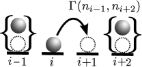
Figure 1: (Color online) Sketch of particle jump with rate $\Gamma(n_{i-1},n_{i+2})$ from site $i$ to site $(i+1)$ for the different possibilities of occupations of sites $(i-1)$ and $(i+2)$.

As mentioned in the Introduction, we here use the widely employed Glauber rates Glauber:1963

$$\Gamma(n_{i-1},n_{i+2}) =\frac{\nu}{2}\left[1-\tanh\left(\frac{\beta\Delta\mathcal{H}}{2}\right)\right]$$

$$=\frac{\nu}{\exp[\beta(n_{i+2}-n_{i-1})V]+1}\,,$$ (5)

where $\nu$ is an attempt frequency, $\beta$ is the inverse thermal energy, and $\Delta\mathcal{H}=(n_{i+2}-n_{i-1})V$ is the energy difference between the states after and before the jump. In the following we set $\beta=1$ and $\nu=1$. Because $\Gamma(0,0)=\Gamma(1,1)$, the bulk dynamics is particle-hole symmetric, i.e. a bulk system with particle concentration $\rho$ and the set of jump rates $\{\Gamma(0,0),\Gamma(1,0),\Gamma(0,1),\Gamma(1,1)\}$ is equivalent to a bulk system with particle concentration $1-\rho$ and the set of jump rates $\{\Gamma(1,1),\Gamma(1,0),\Gamma(0,1),\Gamma(0,0)\}$.

III Bulk current-density relation

To evaluate the bulk current-density relation in NESS, one has to determine the correlators in Eq. (4). In general this is a difficult task because, different from equilibrium systems, there are no universal laws yielding the distributions of microstates in NESS. On the other hand, some authors Katz/etal:1984 ; Singer/Peschel:1980 have considered the question whether it is possible to specify the rates $\Gamma(n_{i-1},n_{i+2})$ in such a way that the distribution of microstates in the NESS equals the equilibrium Boltzmann distribution $\propto\exp(-\mathcal{H})$. Indeed it was found that this is the case, if the rates satisfy the relations

$$\Gamma(0,1)=\Gamma(1,0)\,e^{-V}\,,$$ (6a)

$$\Gamma(0,0)+\Gamma(1,1)-\Gamma(0,1)-\Gamma(1,0)=0\,.$$ (6b)

A derivation of these relations is given in the Appendix, because it was not given in detail in the original work Katz/etal:1984 .

Interestingly, the Glauber rates satisfy Eqs. (6a) and (6b). As a consequence, the correlators in Eq. (4) equal the equilibrium correlators in the corresponding one-dimensional Ising model, which can be calculated by various means, such as the transfer matrix technique, density functional theory etc. The result for the current reads

$$j(\rho) =\left(\rho-C^{(1)}\right)^{2}\,\frac{2f-1}{2\rho(1-\rho)}+\left(\rho-C^{(1)}\right)(1-f)\,,$$ (7)

where $f=1/[\exp(V)+1]=\Gamma(0,1)$ and $C^{(1)}=\langle n_{i}n_{i+1}\rangle_{\rm eq}$ is the equilibrium nearest-neighbor correlator,

$$C^{(1)} =\frac{1}{2(1-e^{-V})}\bigg{[}2\rho(1-e^{-V})-1\bigg{.}$$

$${}+\bigg{.}\sqrt{1-4\rho(1-\rho)(1-e^{-V})}\bigg{]}\,.$$ (8)

Because the bulk dynamics is particle-hole symmetric, $j(\rho)=j(1-\rho)$.

Figure 2 shows the behavior of the current as a function of density for various interaction strength $V$. For $V\to 0$, $j(\rho)$ approaches the parabola $j=(\rho-\rho^{2})/2$ for particles with site exclusion only. When $V$ exceeds a critical value $V_{\star}=2\ln 3\simeq 2.20$, $j(\rho)$ develops a double-hump structure Dieterich/etal:1980 ; Krug:1991 with two maxima at densities

$$\rho_{1,2}^{*}(V) =\frac{1}{2}\mp\sqrt{\frac{3}{4}-\frac{1}{2}\sqrt{\frac{2e^{V}}{e^{V}-1}}}\,,$$ (9)

and a minimum at half-filling, i.e., for $\rho=1/2$. In the limit case $V\to\infty$, we find $j=(x^{3/2}-2x+x^{1/2})/(2-2x)$ with $x=(2\rho-1)^{2}$, meaning that there is no particle movement for $\rho=1/2$. For $\rho^{*}_{1,2}=1/2\mp\left(\sqrt{2}-1\right)/2$ the current is maximal, in agreement with earlier findings reported by Krug Krug:1991 .

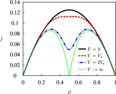
Figure 2: (Color online) Bulk current-density relation $j(\rho)$ for various interaction strengths $V$.

IV Transport in Open System: Application of MCAK

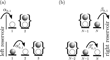
Figure 3: Couplings of the system to the (a) left and (b) right reservoirs mediated by the $\alpha$ and $\beta$ rates. Indices $0$ and $1$ refer to the occupation of the sites next to the target site (for $\alpha$ rates) and to the initial site (for $\beta$ rates). The primed rates are for jumps from and to boundary sites of the system.

Coupling of the TASEP to a left and right reservoir in general requires eight coupling parameters for nearest-neighbor interactions, as indicated in Fig. 3. For injection of particles to site $i=1$, $\alpha_{0}$ and $\alpha_{1}$ specify the injection rates if site $i=2$ is vacant or occupied, respectively. Due to the missing neighbor on the left for particles on site $i=1$, in addition the rates for the two possible jumps from site $i=1$ need to be specified. These are denoted by $\alpha_{0,1}^{\prime}$ for vacant/occupied site $i=3$. Analogously, $\beta_{0,1}$ denote the two possible ejection rates for vacant/occupied site $i=N-1$, and $\beta_{0,1}^{\prime}$ the two possible rates from site $i=N-1$ for vacant/occupied site $i=N-2$.

To evaluate the currents in Eq. (4), we cannot use any longer the mapping of the NESS to an (unbiased) equilibrium state as discussed in the previous Sec. III, because the translational invariance used in the derivation (cf. Appendix) is broken. As known also from the standard TASEP with site exclusion only, the distribution of microstates is not uniform in the open systems, that means it changes when going from the bulk to the open system.

To treat the relevant correlators in Eq. (4) one can consider their time evolutions. This would lead to the appearance of higher-order correlators and different procedures could be applied for closing the resulting hierarchy. However, this approach usually becomes unhandy. Instead we use the underlying concept of TDFT Reinel/Dieterich:1996 ; Heinrichs/etal:2004 ; Dierl/etal:2011 , which is based on the (time-)local equilibrium approximation. This amounts to approximate the non-equilibrium distribution $P(\boldsymbol{n},t)$ by the Boltzmann probability $\propto\exp[-\mathcal{H}(\boldsymbol{n})]$ plus an effective time-dependent external potential $\sum_{i}h_{i}[\boldsymbol{\rho}(t)]n_{i}$, where $\boldsymbol{\rho}(t)=\{\rho_{i}\}$. This implies that the correlators at any time $t$ are supposed to be related to densities as in an equilibrium system. These relations are now needed for inhomogeneous systems without translational invariance. In particular, as mentioned in the Introduction, it is important to include information on the local variation of the density.

To this end the Markov approach for expressing the distribution of microstates Buschle/etal:2000 is particularly suited. In this approach the equilibrium joint probabilities $p^{(j+1)}_{\rm eq}(n_{i},\ldots,n_{i+j})$ for the occupation numbers $n_{i},\ldots,n_{i+j}$ are expressed by the Markov chain $p^{(j+1)}_{\rm eq}(n_{i},\ldots,n_{i+j})=p^{(1)}_{\rm eq}(n_{i})\prod_{s=1}^{j}w(n_{i+s}|n_{i+s-1})$, where $p^{(1)}_{\rm eq}(n_{i})$ is the probability for $n_{i}$ in equilibrium, and $w(n_{i+1}|n_{i})=p^{(2)}_{\rm eq}(n_{i},n_{i+1})/p^{(1)}_{\rm eq}(n_{i})$ is the conditional probability for $n_{i+1}$ given $n_{i}$. Since the joint probabilities are directly connected to the correlators, e.g., $p^{(4)}_{\rm eq}(n_{i-1}\!=\!0,n_{i}\!=\!1,n_{i+1}\!=\!0,n_{i+2}\!=\!0)=\langle\tilde{n}_{i-1}n_{i}\tilde{n}_{i+1}\tilde{n}_{i+2}\rangle_{\rm eq}$, all four-point correlators in Eq. (4) can thus be reduced to two-point correlators.

Applying this MCAK procedure to the TASEP with nearest-neighbor interactions yields

$$j_{i,i+1} =\frac{C_{i}^{(2)}}{\rho_{i}(1\!-\!\rho_{i+1})}$$

$${}\times\left(C_{i-1}^{(3)}C_{i+1}^{(4)}\Gamma(0,0)+C_{i-1}^{(1)}C_{i+1}^{(4)}\Gamma(1,0)\right.$$

$$\hskip 10.00002pt\left.{}+C_{i-1}^{(3)}C_{i+1}^{(3)}\Gamma(0,1)+C_{i-1}^{(1)}C_{i+1}^{(3)}\Gamma(1,1)\right)\,,$$ (10)

where

$$C_{i}^{(2)} =\langle n_{i}\tilde{n}_{i+1}\rangle_{\rm eq}=\rho_{i}-C_{i}^{(1)}\,,$$ (11a)

$$C_{i}^{(3)} =\langle\tilde{n}_{i}n_{i+1}\rangle_{\rm eq}=\rho_{i+1}-C_{i}^{(1)}\,,$$ (11b)

$$C_{i}^{(4)} =\langle\tilde{n}_{i}\tilde{n}_{i+1}\rangle_{\rm eq}=1-\rho_{i}-\rho_{i+1}+C_{i}^{(1)}\,,$$ (11c)

and $C_{i}^{(1)}$ follows from the quadratic equation

$$C_{i}^{(1)} =e^{-V}\frac{\left(\rho_{i}-C_{i}^{(1)}\right)\left(\rho_{i+1}-C_{i}^{(1)}\right)}{1-\rho_{i}-\rho_{i+1}+C_{i}^{(1)}}\,.$$ (12)

Selecting the physical branch of the solution, we obtain

$$C_{i}^{(1)}=\frac{1}{2(1-e^{-V})}\bigg{[}(\rho_{i}+\rho_{i+1})(1-e^{-V})-1\bigg{.}$$

$$+\bigg{.}\sqrt{\left[(\rho_{i}+\rho_{i+1})(1-e^{-V})-1\right]^{2}+4\rho_{i}\rho_{i+1}e^{-V}(1-e^{-V})}\bigg{]}\,.$$ (13)

In addition to the currents $j_{i,i+1}$ not directly coupled to the injection and ejection rate, we need the currents at the boundary sites,

$$j_{{\rm\scriptscriptstyle L},1} =\langle\tilde{n}_{1}\tilde{n}_{2}\rangle\alpha_{0}+\langle\tilde{n}_{1}n_{2}\rangle\alpha_{1}\,,$$ (14a)

$$j_{1,2} =\langle n_{1}\tilde{n}_{2}\tilde{n}_{3}\rangle\alpha_{0}^{\prime}+\langle n_{1}\tilde{n}_{2}n_{3}\rangle\alpha_{1}^{\prime}\,,$$ (14b)

$$j_{N,{\rm\scriptscriptstyle R}} =\langle\tilde{n}_{N-1}n_{N}\rangle\beta_{0}+\langle n_{N-1}n_{N}\rangle\beta_{1}\,,$$ (14c)

$$j_{N-1,N} =\langle\tilde{n}_{N-2}n_{N-1}\tilde{n}_{N}\rangle\beta_{0}^{\prime}$$

$$\hskip 10.00002pt{}+\langle n_{N-2}n_{N-1}\tilde{n}_{N}\rangle\beta_{1}^{\prime}\,.$$ (14d)

Using the method outlined above, we obtain

$$j_{{\rm\scriptscriptstyle L},1} =C_{1}^{(4)}\alpha_{0}+C_{1}^{(3)}\alpha_{1},$$ (15a)

$$j_{1,2} =\frac{C_{1}^{(2)}}{1-\rho_{2}}\left(C_{2}^{(4)}\alpha_{0}^{\prime}+C_{2}^{(3)}\alpha_{1}^{\prime}\right)\,,$$ (15b)

$$j_{N,{\rm\scriptscriptstyle R}} =C_{N-1}^{(3)}\beta_{0}+C_{N-1}^{(1)}\beta_{1}\,,$$ (15c)

$$j_{N-1,N} =\frac{C_{N-1}^{(2)}}{\rho_{N-1}}\left(C_{N-2}^{(3)}\beta_{0}^{\prime}+C_{N-2}^{(1)}\beta_{1}^{\prime}\right)\,.$$ (15d)

Given the explicit expressions (IV), (15) for the currents in terms of the densities via Eqs. (11), (12) the kinetic equations (2) become a closed set.

V Boundary-induced NESS phases

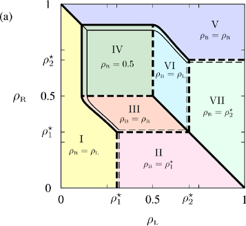
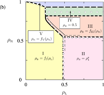
Figure 4: (Color online) Boundary-induced phase diagrams of NESS at $V=2V_{\star}$ for (a) the bulk-adapted and (b) the equilibrated-bath couplings. Thick solid and thick dashed lines mark first- and second-order phase transitions for the TASEP. Corresponding thin lines are for the ASEP with $F=2$. In (b) the symbols refer to KMC results and the lines to MCAK results.

As mentioned in the Introduction, applicability of the minimum and maximum current principles requires specific “bulk-adapted couplings” of the system to the reservoirs. In fact, the $\alpha$ and $\beta$ rates need to be defined in such a way that the system can be viewed as being continued into the reservoirs, corresponding to relations between correlators and densities as in the bulk.

In a bulk system, when an initial configuration $\{n_{i+1}=0,n_{i+2}\}$ would be given, two rates are possible for a particle jump from site $i$ (i.e. $n_{i}=1$): $\Gamma_{i,i+1}=1/[\exp(n_{i+2}V)+1]$, if $n_{i-1}=0$, while $\Gamma_{i,i+1}=1/[\exp(n_{i+2}V-V)+1]$, if $n_{i-1}=1$. For given $\{n_{i+1}=0,n_{i+2}\}$, let us denote by $p(01|0n_{i+2};\rho)=p(010n_{i+2};\rho)/p(0n_{i+2};\rho)$ and $p(11|0n_{i+2};\rho)=p(110n_{i+2};\rho)/p(0n_{i+2};\rho)$ the conditional probabilities for the configurations $\{n_{i-1},n_{i}\}=\{0,1\}$ and $\{n_{i-1},n_{i}\}=\{1,1\}$ to occur in the NESS of a closed bulk system with density $\rho$ and interaction $V$. For example, injection rate $\alpha_{0,1}$ then results from a weighting of rates with the probabilities $p(01|0n_{2};\rho_{\rm\scriptscriptstyle L})$ and $p(11|0n_{2};\rho_{\rm\scriptscriptstyle L})$ corresponding to virtual configurations $\{n_{-1}=0,n_{0}=1,n_{1}=0,n_{2}\}$ and $\{n_{-1}=1,n_{0}=1,n_{1}=0,n_{2}\}$ at the boundaries. Following the same procedure for the other rates we arrive at ($m=0$ or 1)

$$\alpha_{m} =\frac{p(01|0m;\rho_{\rm\scriptscriptstyle L})}{\exp(mV)+1}+\frac{p(11|0m;\rho_{\rm\scriptscriptstyle L})}{\exp[(m-1)V]+1}\,,$$ (16a)

$$\alpha_{m}^{\prime} =\frac{p(0|10m;\rho_{\rm\scriptscriptstyle L})}{\exp(mV)+1}+\frac{p(1|10m;\rho_{\rm\scriptscriptstyle L})}{\exp[(m-1)V]+1}\,,$$ (16b)

$$\beta_{m} =\frac{\bar{p}(00|1m;\rho_{\rm\scriptscriptstyle R})}{\exp(-mV)+1}+\frac{\bar{p}(10|1m;\rho_{\rm\scriptscriptstyle R})}{\exp[(1-m)V]+1}\,,$$ (16c)

$$\beta_{m}^{\prime} =\frac{\bar{p}(0|01m;\rho_{\rm\scriptscriptstyle R})}{\exp(-mV)+1}+\frac{\bar{p}(1|01m;\rho_{\rm\scriptscriptstyle R})}{\exp[(1-m)V]+1}\,.$$ (16d)

Here, $p(0|10m;\rho)$ and $p(1|10m;\rho)$ are, respectively, the bulk probabilities for $n_{i-1}=0$ and $n_{i-1}=1$ under the condition that $\{n_{i},n_{i+1},n_{i+2}\}=\{1,0,m\}$. Note that for the $\beta$ rates the given occupation numbers are those to the left side, i.e. $\bar{p}(00|1m;\rho)=p(m100;\rho)/p(m1;\rho)$ and so on.

Application of the minimum and maximum current principles to the TASEP with $V=2V_{\star}$ and the bulk-adapted rates in Eqs. (16) yields the boundary-induced phase diagram shown in Fig. 4(a). In total seven phases occur, where the bulk density equals either the left reservoir density $\rho_{\rm\scriptscriptstyle L}$ (phases I and VI), or the right reservoir density $\rho_{\rm\scriptscriptstyle R}$ (phases III and V), or the densities $\rho_{1,2}^{\star}$ [see Eq. (9)] of maxima in the current (phases II and VII), or the density 0.5 of the (local) minimum in the current (phase IV). Transitions between these phases can be of first or second order, which are indicated by thick solid and thick dashed lines, respectively. The thin lines refer to changes of the phase diagram when allowing for jumps against the bias direction, as further discussed in Sec. VII. Notice that the diagram has symmetry with respect to the diagonal $\rho_{\rm\scriptscriptstyle R}=1-\rho_{\rm\scriptscriptstyle L}$, which reflects the particle-hole symmetry in the system as explained in the following Sec. VI.

The results for the bulk densities and currents of the NESS in the case of bulk-adapted couplings and for our choice of rates satisfying the relations (6) are exact. Note that this does not hold true for the density profile close to the boundaries. Application of the MCAK described in Sec. IV allows one also to calculate the time evolution of density profiles. Corresponding numerical solutions of Eq. (2) with the expressions for the currents derived in Sec. IV are approximate both at the boundaries and in the bulk, because at transient times the relations between correlators and densities differ from those in the equilibrium state without bias.

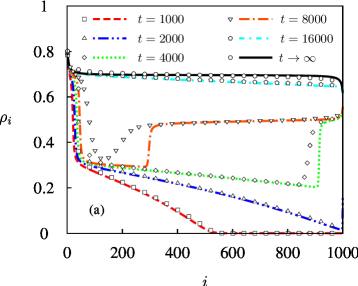
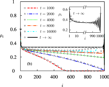
Figure 5: (Color online) Time evolution of $\rho_{i}$ for (a) bulk-adapted and (b) equilibrated-bath couplings of the systems to the reservoirs for $\rho_{\rm\scriptscriptstyle L}=0.9$, $\rho_{\rm\scriptscriptstyle R}=0.6$, $V=2V_{\star}$, $N=1000$, and $\rho_{i}(t=0)=0$. KMC results are marked by symbols and MCAK results by lines. In the KMC simulations, averages were performed over $10^{6}$ different configurations. The inset in (b) zooms out the oscillatory behavior at the boundaries.

In order to get insight how well the MCAK captures the kinetics, we have performed kinetic Monte Carlo (KMC) simulations of the TASEP with bulk-adapted couplings for a chain of $N=1000$ sites with $\rho_{\rm\scriptscriptstyle L}=0.9$, $\rho_{\rm\scriptscriptstyle R}=0.6$, $V=2V_{\star}$ and an initially empty lattice. Results from these KMC simulations (symbols) for density profiles at five different times, as well as the stationary state, are compared in Fig. 5(a) with the predictions of the MCAK (lines). Three different time regimes can be distinguished. The first regime is the “penetration regime” for $t\lesssim 2000$ during which the initially injected particles pass the system and reach the right reservoir. In this regime there is excellent agreement of the KMC data with the MCAK predictions. The penetration regime is followed by an “intermediate regime”, where the density in the system increases until approaching values close to the limiting one in the NESS. The two times $t=4000$ and $t=8000$ in Fig. 5(a) belong to this regime. For the choice of parameters in the present example, it is interesting that a kind of domain wall appears in the system, see the jump-like change of density at $i\approx 900$ for $t=4000$ that has moved to $i\approx 200$ for $t=8000$. A second such kind of domain wall appears in the time interval 8000 and 16000 and moves to the right (not shown).

One can view the occurrence of these transient domain walls as resembling the occurrence of domain walls along first-order lines in the phase diagrams of the NESS. Contrary to the latter, the positions of the transient walls not only fluctuate, but they exhibit an average drift, because the local current in the system is not constant. For the wall seen in Fig. 5(a), the current left to the wall must on average be larger than right to the wall. The MCAK captures the formation of transient domain walls, but the quantitative agreement with the KMC data is less accurate than in the penetration regime. The intermediate regime is followed by a “relaxation regime”, where at each point the density continuously relaxes, without rapid jump-like changes, towards the limiting value in the NESS. In this regime the MCAK predictions are again in excellent agreement with the KMC data.

The bulk-adapted couplings are specifically tuned to make the minimum and maximum current principles applicable. With respect to applications such couplings will not be realized, but one is led by the fact that the time scale of relaxation processes in the reservoirs is much faster than in the system. With this assumption, baths can be assumed to correspond to equilibrated Fermi gases with chemical potentials $\mu_{\rm\scriptscriptstyle L}=\ln[\rho_{\rm\scriptscriptstyle L}/(1-\rho_{\rm\scriptscriptstyle L})]$ and $\mu_{\rm\scriptscriptstyle R}=\ln[\rho_{\rm\scriptscriptstyle R}/(1-\rho_{\rm\scriptscriptstyle R})]$. A reasonable ansatz for the $\alpha$ and $\beta$ rates then is

$$\alpha_{m} =\rho_{\rm\scriptscriptstyle L}[\exp(mV-\mu_{\rm\scriptscriptstyle L})+1]^{-1}\,,$$ (17a)

$$\alpha_{m}^{\prime} =[\exp(mV)+1]^{-1}\,,$$ (17b)

$$\beta_{m} =(1-\rho_{\rm\scriptscriptstyle R})[\exp(\mu_{\rm\scriptscriptstyle R}-mV)+1]^{-1}\,,$$ (17c)

$$\beta_{m}^{\prime} =[\exp(-mV)+1]^{-1}\,.$$ (17d)

The Fermi factors in these rates correspond to the Glauber rates, if one considers that injected particles loose an energy $\mu_{\rm\scriptscriptstyle L}$, ejected particles gain an energy $\mu_{\rm\scriptscriptstyle R}$, and that the interaction with particles in the system is as in the bulk. The additional factors $\rho_{\rm\scriptscriptstyle L}$ in Eq. (17a) and $1-\rho_{\rm\scriptscriptstyle R}$ in in Eq. (17c) take into account the filling of the baths. The functional form in Eq. (17) resembles forms resulting from Fermi’s golden rule for transition rates Roche/etal:2005 ; Nitzan:2006 ; Harbola/etal:2006 ; Cuevas/Scheer:2010 . We will refer to the couplings mediated by the rates in Eq. (17) as the “equilibrated-bath couplings”.

For these couplings, the density profiles at the boundaries can no longer be expected to vary monotonically, as it is required for applicability of the minimum and maximum current principles. Considering equilibrium systems, it is well known that modified interactions, for example at confining walls, commonly lead to density oscillations. It would be surprising if such density oscillations do not appear for NESS under modified interactions at the boundaries, as for the equilibrated-bath couplings.

Figure 5(b) shows the time evolution of density profiles obtained from KMC simulations (symbols) and the MCAK (lines) for the same reservoir densities and coupling strength as in Fig. 5(a). Indeed, density oscillations appear at the walls in the stationary state, as demonstrated in the inset of Fig. 5(b). They can be understood when pointing out that the oscillations are missing in the bulk due to translational invariance. If one would, in the bulk, determine the spatial dependence of the density with respect to an occupied site, which in fact amounts to a determination of density correlations, then it is clear that oscillations occur due to the repulsive nearest-neighbor interactions. The same holds true when the spatial dependence of density profiles is determined by starting from a vacant site. The reservoir in case of the equilibrated-bath couplings resembles a vacant site (missing nearest neighbors) and therefore oscillations appear at the boundary. In agreement with this picture, the density at site $N$ next to the right reservoir is particularly large, the density at the next site $N-1$ to the left then particularly low, and this alternating behavior continues on the scale of the correlation length towards the bulk. The bulk density is $\rho_{\rm\scriptscriptstyle B}\cong 0.34$ and deviates from the bulk density $\rho_{\rm\scriptscriptstyle B}\cong 0.70$ in Fig. 5(a) following from the maximum current principle.

To cope with the oscillations a theory is needed where the local current $j_{i,i+1}$ is dependent on the form of the density profile around sites $i$ and $i+1$, as it is the case in the MCAK. As can be seen from Fig. 5(b), the density oscillations at the boundaries are well accounted for by the MCAK, and accordingly the predicted bulk density is in excellent agreement with that from the KMC simulations. Also the time evolution of the density profiles is well captured by the MCAK in Fig. 5(b). Let us note that the breakdown of the minimum and maximum current principles does not imply that phases corresponding to the local minimum and to the maxima in the bulk current density relation can no longer appear. In fact, starting from the flat region and considering the onset of the bending of the profile at the ends of this region, an enlarged region of monotonically varying density profile could be considered, where the minimum and maximum current principles apply.

The boundary-induced phase diagram for $V=2V_{\star}$ and the equilibrated bath couplings is displayed in Fig. 4(b). This diagram strongly differs from the corresponding one for the bulk-adapted couplings in Fig. 4(a). Instead of seven phases, five phases appear, where the bulk density either is determined by the left reservoir density $\rho_{\rm\scriptscriptstyle L}$ via a function $f_{\rm I}(\rho_{\rm\scriptscriptstyle L})$ (phase I), or is determined by the right reservoir density $\rho_{\rm R}$ via functions $f_{\rm III}(\rho_{\rm\scriptscriptstyle R})$ and $f_{\rm V}(\rho_{\rm\scriptscriptstyle R})$ (phases III and V), or is equal to $\rho_{1}^{\star}$ (phase II), or is equal to the density 0.5 of the (local) minimum in the current (phase IV). Analogous to Fig. 4(a), first- and second-order transitions are marked by thick solid and thick dashed lines, respectively. Phases in Fig. 4(a) and (b) labelled by the same Roman numbers correspond to each other in the sense that their character agrees (left or boundary determined, or minimum or maximum current phases). In addition, the phase diagram in Fig. 4(b) is not symmetric with respect to the diagonal $\rho_{\rm\scriptscriptstyle R}=1-\rho_{\rm\scriptscriptstyle L}$. The reason for this will be clarified in the following Sec. VI.

VI Particle-hole symmetry

Under exchange of particles by holes the ejection rates $\beta_{0}$, $\beta_{1}$, $\beta_{0}^{\prime}$, $\beta_{1}^{\prime}$ would correspond to injection rates $\alpha_{1}$, $\alpha_{0}$, $\alpha_{1}^{\prime}$, $\alpha_{0}^{\prime}$, respectively, and the current direction would be reversed. Because the bulk dynamics is particle-hole symmetric, the particle-hole exchanged system must have the same properties with respect to the hole occupation numbers $\tilde{n}_{i}=1-n_{i}$, i.e. densities $\tilde{\rho}_{i}(t)=\langle\tilde{n}_{i}\rangle_{t}$ and correlators $\langle\tilde{n}_{i}\tilde{n}_{j}\tilde{n}_{k}\ldots\rangle_{t}$ at any time $t$ in the particle-hole exchanged system equal $\rho_{i}(t)=\langle n_{i}\rangle_{t}$ and $\langle n_{k}n_{j}n_{i}\ldots\rangle_{t}$ in the original system. In this sense particle-hole symmetry holds true in general.

The bulk density in particular must fulfill in the NESS

$$\rho_{\rm\scriptscriptstyle B}(\alpha_{0},\alpha_{1},\alpha_{0}^{\prime},\alpha_{1}^{\prime},\beta_{0},\beta_{1},\beta_{0}^{\prime},\beta_{1}^{\prime})$$ (18)

$$\hskip 50.00008pt{}=1-\rho_{\rm\scriptscriptstyle B}(\beta_{1},\beta_{0},\beta_{1}^{\prime},\beta_{0}^{\prime},\alpha_{1},\alpha_{0},\alpha_{1}^{\prime},\alpha_{0}^{\prime})\,.$$

For compact notation, let us introduce multivariate $\tilde{\alpha}$ and $\tilde{\beta}$ jump rates under particle-hole exchange of the $\alpha=(\alpha_{0},\alpha_{1},\alpha_{0}^{\prime},\alpha_{1}^{\prime})$ and $\beta=(\alpha_{0},\alpha_{1},\alpha_{0}^{\prime},\alpha_{1}^{\prime})$ rates,

$$\tilde{\alpha}\equiv(\alpha_{1},\alpha_{0},\alpha_{1}^{\prime},\alpha_{0}^{\prime})\,,\qquad\tilde{\beta}\equiv(\beta_{1},\beta_{0},\beta_{1}^{\prime},\beta_{0}^{\prime})\,.$$ (19)

Then we can rewrite Eq. (18) as $\rho_{\rm\scriptscriptstyle B}(\alpha,\beta)=\tilde{\rho}_{\rm\scriptscriptstyle B}(\tilde{\beta},\tilde{\alpha})=1-\rho_{\rm\scriptscriptstyle B}(\tilde{\beta},\tilde{\alpha})$.

Following the view that the reservoirs are controlled by only a few variables, as their chemical potentials or densities, we should require the injection and ejection rates to depend on $\rho_{\rm\scriptscriptstyle L}$ and $\rho_{\rm\scriptscriptstyle R}$, respectively. Given $\alpha=\alpha(\rho_{\rm\scriptscriptstyle L})$ and $\beta=\beta(\rho_{\rm\scriptscriptstyle R})$, the bulk density becomes a function of $\rho_{\rm\scriptscriptstyle L}$ and $\rho_{\rm\scriptscriptstyle R}$,

$$\hat{\rho}_{\rm\scriptscriptstyle B}(\rho_{\rm\scriptscriptstyle L},\rho_{\rm\scriptscriptstyle R}) \equiv\rho_{\rm\scriptscriptstyle B}(\alpha(\rho_{\rm\scriptscriptstyle L}),\beta(\rho_{\rm\scriptscriptstyle R}))\,.$$ (20)

Particle-hole symmetry would show up in this function, if the relation

$$\hat{\rho}_{\rm\scriptscriptstyle B}(\rho_{\rm\scriptscriptstyle L},\rho_{\rm\scriptscriptstyle R}) =1-\hat{\rho}_{\rm\scriptscriptstyle B}(1-\rho_{\rm\scriptscriptstyle R},1-\rho_{\rm\scriptscriptstyle L})$$ (21)

is fulfilled. Replacing the left hand side with $\hat{\rho}_{\rm\scriptscriptstyle B}(\rho_{\rm\scriptscriptstyle L},\rho_{\rm\scriptscriptstyle R})=\rho_{\rm\scriptscriptstyle B}(\alpha(\rho_{\rm\scriptscriptstyle L}),\beta(\rho_{\rm\scriptscriptstyle R}))=1-\rho_{\rm\scriptscriptstyle B}(\tilde{\beta}(\rho_{\rm\scriptscriptstyle R}),\tilde{\alpha}(\rho_{\rm\scriptscriptstyle L}))$ by using Eq. (18), and the right hand side by $1-\hat{\rho}_{\rm\scriptscriptstyle B}(1-\rho_{\rm\scriptscriptstyle R},1-\rho_{\rm\scriptscriptstyle L})=1-\rho_{\rm\scriptscriptstyle B}(\alpha(1-\rho_{\rm\scriptscriptstyle R}),\beta(1-\rho_{\rm\scriptscriptstyle L}))$, we obtain by comparison

$$\alpha(\rho)=\tilde{\beta}(\tilde{\rho})$$ (22)

as the condition for the particle-hole symmetry in Eq. (21) to be obeyed.

The rates in Eqs. (17) for the equilibrated-bath couplings do not satisfy relation (22) and hence the phase diagram in Fig. 4(b) does not display the symmetry according to Eq. (21). For the bulk-adapted couplings, in contrast, the rates in Eq. (16) satisfy Eq. (22). For example, $\beta_{1}(1-\rho)=(\exp(-V)+1)^{-1}p(1100;1-\rho)/p(11;1-\rho)+2^{-1}p(1101;1-\rho)/p(11;1-\rho)=(\exp(-V)+1)^{-1}p(1100;\rho)/p(00;\rho)+2^{-1}p(0100;\rho)/p(00;\rho)=\alpha_{0}$, where we have used the particle-hole symmetry $p(n_{i-1},n_{i},n_{i+1},n_{i+2};1-\rho)=p(\tilde{n}_{i-1},\tilde{n}_{i},\tilde{n}_{i+1},\tilde{n}_{i+2};\rho)$ in the bulk. Analogously, the other relations in Eq. (22) can be proven.

Theoretically, given the particle-hole symmetric bulk dynamics, the behavior in the open system is fully controlled by the eight $\alpha$ and $\beta$ jump rates, and the different boundary-induced phases would appear in a particle-hole symmetric manner in the respective eight-dimensional space. However, in practice it will be difficult to “control” couplings in this detailed way. Rather the system will be connected somehow to the reservoirs and one could tune the reservoir properties. In the case considered here, this is reflected by Eq. (20), which parameterizes the eight rates in terms of two densities. As a consequence, different phases from the eight-dimensional space are projected out into the $(\rho_{\rm\scriptscriptstyle L},\rho_{\rm\scriptscriptstyle R})$-plane for different coupling mechanisms. This can go along with significant changes of the topology, as indeed obtained in Fig. 4.

VII ASEPs

TASEPs are simplified models because jumps against the bias direction are not included. For hard-core exclusions only, it is known that the structure of the boundary-induced phase remains essentially the same when allowing for backward jumps Sandow:1994 ; Kolomeisky/etal:1998 . In the presence of a bias $F$ in forward direction, forward and backward jump rates $\Gamma_{\rightarrow}$ and $\Gamma_{\leftarrow}$ are generally assumed to fulfill the detailed balance condition, i.e. $\Gamma_{\rightarrow}/\Gamma_{\leftarrow}=\exp(-\Delta\mathcal{H})$, where the lattice gas Hamiltonian in the presence of the bias reads

$$\mathcal{H}=V\sum_{i}n_{i}n_{i+1}-F\sum_{i}i\,n_{i}\,.$$ (23)

Considering a corresponding ASEP in the limit $F\to\infty$, an associated TASEP with rates $\Gamma=\lim_{F\to\infty}\Gamma_{\rightarrow}$ is obtained, if the forward rates saturate for infinite bias. Conversely, given a TASEP with rates $\Gamma$, an ASEP can be defined that in the limit $F\to\infty$ reduces to the TASEP, for example, by setting $\Gamma_{\rightarrow}=\Gamma$ independent of $F$ and $\Gamma_{\leftarrow}=\Gamma\exp(-\Delta\mathcal{H})$.

Interestingly, TASEPs can even be associated with ASEPs in the linear response regime of weak bias $F$. Let us consider an ASEP with the Glauber rates from Eq. (II), where the forward jump rate is now given by

$$\Gamma_{\rightarrow}(n_{i-1},n_{i+2}) =\frac{1}{e^{(n_{i+2}-n_{i-1})V-F}+1}\,,$$ (24)

and the backward jump rate by $\Gamma_{\leftarrow}(n_{i-1},n_{i+2})=\Gamma_{\rightarrow}(n_{i-1},n_{i+2})\exp\left[(n_{i+2}-n_{i-1})V-F\right]$. Because the $\Gamma_{\rightarrow}(n_{i-1},n_{i+2})$ no longer satisfy Eqs. (6), calculations for the bulk behavior in the NESS, based on equilibrium relations between correlators and densities, are not exact. We can expect, however, that the MCAK will provide a good approximation for small bias $F$.

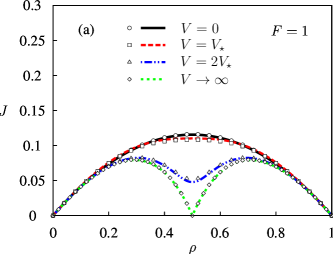
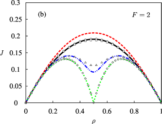
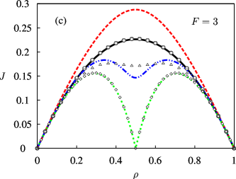
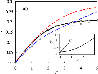
Figure 6: (Color online) (a)-(c) Current-density relations $j(\rho)$ for the ASEP at various $V$ and three different bias strengths $F$. In (d) the current-bias relation is shown for $\rho=0.3$. Symbols refer to KMC data, lines to MCAK results, and the assignment of lines and symbols to the different interaction strength $V$ is given in the legend of (a).

The forward current $j_{i,i+1}$ from site $i$ to site $i+1$ has the same form as in Eq. (IV) with the jump rates given by Eq. (24). The backward current $j_{i+1,i}$ follows from interchanging $\rho_{i}$ and $\rho_{i+1}$, and the indices $(i-1)$ and $(i+1)$ as well as the superscripts $(2)$ and $(3)$ in the correlators,

$$j_{i+1,i} =\frac{C_{i}^{(3)}}{\rho_{i+1}(1\!-\!\rho_{i})}$$ (25)

$${}\times\left(C_{i+1}^{(2)}C_{i-1}^{(4)}\Gamma_{\leftarrow}(0,0)+C_{i+1}^{(1)}C_{i-1}^{(4)}\Gamma_{\leftarrow}(0,1)\right.$$

$$\hskip 10.00002pt\left.{}+C_{i+1}^{(2)}C_{i-1}^{(2)}\Gamma_{\leftarrow}(1,0)+C_{i+1}^{(1)}C_{i-1}^{(2)}\Gamma_{\leftarrow}(1,1)\right)\,.$$

Except that the $j_{i,i+1}$ must be replaced by the net currents

$$J_{i,i+1}(t)=j_{i,i+1}(t)-j_{i+1,i}(t)$$ (26)

between sites $i$ and $i+1$, the rate equations (2) remain the same.

Bulk current-density relations in the NESS from the MCAK are compared to KMC results in Fig. 6(a)-(c) for various interaction strengths $V$ and three different bias values $F=1$, 2 and 3. As expected, for small $F=1$ [Fig. 6(a)], the MCAK gives excellent agreement with the KMC simulations for all $V$. With increasing $F$, deviations become significant for $F\gtrsim V$, see, for example, the results for $V=V_{\star}$ and $F=3$ in Fig. 6(c). Note, however, that for the special case $V=0$, corresponding to the standard ASEP with hard-core exclusion only, the MCAK always gives exact results, independent of $F$, because in this case all microstates are equally probable Derrida:1998 . In the regime of strong interactions $V>F$, the MCAK provides good results, and in particular agrees with the KMC results in the limit $V\to\infty$.

The current as a function of the bias $F$ is shown in Fig. 6(d) for one representative particle density $\rho_{\rm\scriptscriptstyle B}=0.3$ and three different values $V=0$, $V_{\star}$ and $2V_{\star}$. For $F\lesssim 1$, the current increases linearly with $F$, while for $F\gtrsim 1$ nonlinear response effects become relevant. For large $F$, the currents from the KMC simulations saturate at values independent of $V$, while the limiting currents in the MCAK are $V$-dependent. The critical values $V_{c}(F)$, where the bulk-current density relation develops a double-hump structure, see Figs. 6(a)-(c), increase with stronger bias. In the inset of Fig. 6(d), we display the MCAK results for $V_{c}(F)$. Surprisingly, for $F\to 0$, where the MCAK becomes accurate, $V_{c}(F)$ approaches the critical value $V_{\star}$ for the TASEP considered in Sec. II.

To understand this, let us write the net current as

$$J =p(0100)\Gamma_{\rightarrow}(0,0)-p(0010)\Gamma_{\leftarrow}(0,0)$$

$${}+p(1100)\Gamma_{\rightarrow}(1,0)-p(0011)\Gamma_{\leftarrow}(0,1)$$

$${}+p(0101)\Gamma_{\rightarrow}(0,1)-p(1010)\Gamma_{\leftarrow}(1,0)$$

$${}+p(1101)\Gamma_{\rightarrow}(1,1)-p(1011)\Gamma_{\leftarrow}(1,1)$$ (27)

where we have combined in each line “reversed configurations”, i.e. equivalent situations for forward and backward jumps. The $p(....)$ are independent of $F$ in the MCAK (in the bulk) and the same for a given configuration and its reversed. Hence we can rewrite Eq. (27) in a way that in each line the first $p(....)$ are multiplied by the differences $\Gamma_{\rightarrow}(.,.)-\Gamma_{\leftarrow}(.,.)$ between forward and backward rates. Taking the linear response limit of these differences gives $J=Fj_{\rm\scriptscriptstyle TASEP}+\mathcal{O}(F^{2})$, where $j_{\rm\scriptscriptstyle TASEP}$ refers to a TASEP with rates

$$\Gamma(n_{i-1},n_{i+2})=\frac{1}{1+\cosh[(n_{i+2}-n_{i-1})V]}\,.$$ (28)

Again these rates do not satisfy Eq. (6), implying that the MCAK treatment of the bulk NESS behavior of this TASEP is no longer exact. Although the rates in Eqs. (28) and (II) are different, the MCAK yields the same current-density relation given in Eq. (7). Accordingly, $V_{c}(F)$ becomes $V_{\star}$ in the limit $F\to 0$.

That in the MCAK, the ASEP in the linear response regime can be associated with a TASEP raises the question whether this would be true in an exact treatment. Considering a general expansion of the right hand side of Eq. (27) for small $F$, this requires the $p(....)$ to exhibit no linear terms in $F$. We have not yet achieved to prove this property, but representative KMC results shown in Fig. 7 for the $p(....)$ in the second line of Eq. (27) are in agreement with it.

Let us now extend our discussion to open systems. The functional form of the boundary currents in bias direction are as in Eqs. (15a)-(15d) with the $\alpha$ and $\beta$ rates replaced by $\alpha_{\rightarrow}$ and $\beta_{\rightarrow}$ rates. The backward currents are

$$j_{1,{\rm\scriptscriptstyle L}} =C_{1}^{(2)}\alpha_{\leftarrow,0}+C_{1}^{(1)}\alpha_{\leftarrow,1}\,,$$ (29a)

$$j_{2,1} =\frac{C_{1}^{(3)}}{\rho_{2}}\left(C_{2}^{(2)}\alpha_{\leftarrow,0}^{\prime}+C_{2}^{(1)}\alpha_{\leftarrow,1}^{\prime}\right)\,,$$ (29b)

$$j_{{\rm\scriptscriptstyle R},N} =C_{N-1}^{(4)}\beta_{\leftarrow,0}+C_{N-1}^{(2)}\beta_{\leftarrow,1}\,,$$ (29c)

$$j_{N,N-1} =\frac{C_{N-1}^{(3)}}{1-\rho_{N-1}}\left(C_{N-2}^{(4)}\beta_{\leftarrow,0}^{\prime}+C_{N-2}^{(2)}\beta_{\leftarrow,1}^{\prime}\right)\,.$$ (29d)

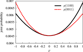
Figure 7: (Color online) KMC results for the joint probabilities $p(1100)$ and $p(0011)$ of finding a configuration $\{n_{i-1}=1,n_{i}=1,n_{i+1}=0,n_{i+2}=0\}$ and its reversed configuration $\{n_{i-1}=0,n_{i}=0,n_{i+1}=1,n_{i+2}=1\}$ in the bulk part of the NESS for the ASEP defined in Eq. (24). The interaction strength is $V=2V_{\star}$ and the particle concentration $\rho=0.5$.

As discussed above, the MCAK provides an accurate description in the linear response regime, and the bulk behavior of the ASEP in this regime is equivalent to a TASEP with rates (28). Moreover, the MCAK predicts the same bulk-density relation for the rates (28) as for the rates (II). Accordingly, it is insightful to compare the boundary-induced phase diagrams of the ASEP with the TASEP in Sec. II.

To this end we have, for the bulk-adapted coupling, applied the minimum and maximum current principles to the bulk current-density relations of ASEPs for various $F$ at $V=2V_{\star}$, as, for example, to those shown Fig. 6(a)-(c). For the equilibrated-bath couplings we use Eqs. (17) for the $\alpha_{\rightarrow}$, $\beta_{\rightarrow}$ rates with $\mathcal{H}$ from Eq. (23) and $\alpha_{\leftarrow}$, $\beta_{\leftarrow}$ rates determined by the detailed balance condition. The corresponding rate equations are integrated numerically for various $F$ at $V=2V_{\star}$ and the resulting density profiles analyzed in the long-time limit.

For small $F\to 0$, we found that MCAK results for the phase diagrams in Figs. 4(a) and (b) are almost the same for the ASEP. Visible small differences appear when $F$ leaves the linear response regime. To illustrate this, we have indicated in both Figs. 4(a) and (b) phase transitions (thin solid and dashed lines) for $F=2$.

VIII Conclusions

Effects of interparticle interactions beyond hard-core exclusions in collective driven transport pose many challenges and possibilities, whose significance has not yet fully explored. Here we have considered ASEPs and TASEPs with repulsive nearest-neighbor interactions in one dimension. For these jump processes on lattices, currents can in general be expressed in terms of correlators of occupation numbers whose order increases with the interaction range. To arrive at closed sets of kinetic equations, one has to decide on how to treat the relevant correlations. The Markov chain approach for deriving exact density functionals Buschle/etal:2000 allows one to express correlators in terms of densities, where the respective relations, strictly valid in equilibrium, entail information on the local density variation, which is necessary to capture interaction-induced non-monotonic behavior of density profiles. Let us note that a standard TDFT treatment based on an exact functional would provide such relations only via the solution of integral equations connecting the correlators with direct correlation functions.

As we have demonstrated, application of the MCAK leads to a good description of both the time evolution of density profiles and their limiting shape in the NESS. Because of this, boundary-induced phase transitions of the bulk density as functions of reservoir densities could be well predicted. The coupling to the reservoirs turned out to have a decisive influence also on the topology of phase diagrams. Particle-hole symmetry in the nearest-neighbor interacting lattice gas with open boundaries manifests itself in certain relations between the injection and ejection rates. It was clarified under which conditions the particle-hole symmetry shows up also with respect to the reservoir densities in the boundary-induced phase diagrams. Furthermore we have demonstrated that ASEPs in the linear response regime can be mapped onto TASEPs with rates that are related to the first term in an expansion of the difference between forward and backward rates with respect to the bias. As a consequence, no significant changes in boundary-induced phase diagrams occur when connecting ASEPs with weak bias to corresponding TASEPs.

For the jump rates we have used Glauber forms in this work. These were shown to belong to a class, where the distribution of microstates in the NESS is equal to the Boltzmann distribution of the interacting lattice gas without bias. Accordingly, an exact bulk current-density relation in NESS could be derived. We notice that the mapping of a NESS to an equilibrium state without bias would not be possible in higher dimensions for the Glauber rates Katz/etal:1984 .

In Refs. Dierl/etal:2011 ; Dierl/etal:2012 we considered TASEPs with jump rates $\propto\exp(-\Delta\mathcal{H}/2)$, where, as in Eq. (II), $\Delta\mathcal{H}$ is the energy difference between states after and before the jump. Different from the Glauber rates, these rates are not bounded and do not fulfill Eqs. (6a) and (6b). Nevertheless the phase diagrams for bulk-adapted and equilibrated-bath couplings are very similar to the ones displayed in Fig. 4. This suggests that the bulk dynamics has only a weak influence in contrast to the dynamics coupled to the reservoirs. This suggestion is reinforced by the fact that the topology of the phase diagram appears to be the same (for given boundary couplings), even if a bulk dynamics is considered that reflects repulsive nearest-neighbor interactions but does not obey particle-hole symmetry (see Fig. 2 in Ref. Hager/etal:2001 ).

It would be interesting to extend the successful treatment based on the TDFT to higher dimensions. For nearest-neighbor interactions there exists a lattice fundamental measure form of the exact zero and one-dimensional density functionals Lafuente/Cuesta:2005 , which enable an extension of these functionals to higher dimensions. Alternatively, the approach used in Sec. IV can also be generalized to higher dimensions Gouyet/etal:2003 . Based on the resulting approximate functionals one could make contact to previous studies of nearest-neighbor interacting driven lattice gases in two dimensions. In these studies structural patterns in the NESS were found Katz/etal:1984 , as, for example, alternating regions of low and high density for attractive interactions $V<0$, manifesting themselves in backgammon- Boal/etal:1991 or stripe- Hurtado/etal:2003 like structures. For repulsive interactions $V>0$, the bias can induce transitions from an ordered to a disordered state Katz/etal:1984 ; Leung/etal:1989 . The treatment of these phenomena by TDFT should in particular allow one to identify phenomenological parameters in former field-theoretical approaches Leung/etal:1989 ; Boal/etal:1991 by appropriate coarse-graining.

*

Appendix A Derivation of rate conditions in Eq. (6)

The master equation

$$\frac{\partial{P(\mathbf{n},t)}}{\partial t}=\sum_{\mathbf{n^{\prime}}}\left[\Gamma(\mathbf{n}^{\prime}\to\mathbf{n})P(\mathbf{n}^{\prime},t)-\Gamma(\mathbf{n}\to\mathbf{n}^{\prime})P(\mathbf{n},t)\right]$$ (30)

describes the change of the probability $P(\mathbf{n},t)$ of finding state $\mathbf{n}$ at time $t$ due to transitions from and to other states $\mathbf{n}^{\prime}$ with rates $\Gamma(\mathbf{n}^{\prime}\to\mathbf{n})$ and $\Gamma(\mathbf{n}\to\mathbf{n}^{\prime})$, respectively. For the model in Sec. II with nearest-neighbor hopping in the presence of nearest-neighbor interactions, we can write

$$\Gamma(\mathbf{n}\to\mathbf{n}^{\prime})=\sum_{i}n_{i}\tilde{n}_{i+1}\delta_{\mathbf{n}^{\prime},\mathbf{n}^{(i,i+1)}}\Gamma(n_{i-1},n_{i+2})\,,$$ (31)

where $\mathbf{n}^{(i,i+1)}$ is identical to the microstate configuration $\mathbf{n}$ except that the occupation numbers $n_{i}$ and $n_{i+1}$ are interchanged. Inserting this into Eq. (30), the master equation for the stationary state of the TASEP reads

$$0= \sum_{i}\left[\tilde{n}_{i}n_{i+1}P({\boldsymbol{n}}^{(i,i+1)})-n_{i}\tilde{n}_{i+1}P(\boldsymbol{n})\right]\Gamma(n_{i-1},n_{i+2})\,.$$ (32)

Assuming that $P(\boldsymbol{n})\propto\exp\left[-\mathcal{H}(\boldsymbol{n})\right]$ with $\mathcal{H}$ from Eq. (1), $P(\mathbf{n}^{(i,i+1)})/P(\mathbf{n})=\exp[-(n_{i+2}-n_{i-1})V]$, and Eq. (32) becomes

$$0 =\sum_{i}\left[\tilde{n}_{i}n_{i+1}e^{-(n_{i+2}-n_{i-1})V}-n_{i}\tilde{n}_{i+1}\right]\Gamma(n_{i-1},n_{i+2})$$

$$=\left[N_{0010}^{{}^{\mathbf{n}}}-N_{0100}^{{}^{\mathbf{n}}}\right]\,\Gamma(0,0)$$

$$\hskip 5.0pt{}+\left[N_{1010}^{{}^{\mathbf{n}}}\,e^{-V}-N_{1100}^{{}^{\mathbf{n}}}\right]\,\Gamma(1,0)$$

$$\hskip 5.0pt{}+\left[N_{0011}^{{}^{\mathbf{n}}}\,e^{V}-N_{0101}^{{}^{\mathbf{n}}}\right]\,\Gamma(0,1)$$

$$\hskip 5.0pt{}+\left[N_{1011}^{{}^{\mathbf{n}}}-N_{1101}^{{}^{\mathbf{n}}}\right]\,\Gamma(1,1)\,,$$ (33)

where $N_{0100}^{{}^{\mathbf{n}}}=\sum_{i}\tilde{n}_{i-1}n_{i}\tilde{n}_{i+1}\tilde{n}_{i+2}$ is the frequency of the sequence $\{0100\}$ of occupation numbers in the microstate $\mathbf{n}$, and analogous definitions apply for the remaining $N_{....}^{{}^{\mathbf{n}}}$. Replacing all $\tilde{n}_{i}$ by $\tilde{n}_{i}=1-n_{i}$, the eight numbers $N_{....}^{{}^{\mathbf{n}}}$ can be expressed in terms of the six irreducible numbers $N_{11}^{{}^{\mathbf{n}}}=\sum_{i}n_{i-1}n_{i}$, $N_{1\_1}^{{}^{\mathbf{n}}}=\sum_{i}n_{i-1}n_{i+1}$, $N_{111}^{{}^{\mathbf{n}}}=\sum_{i}n_{i-1}n_{i}n_{i+1}$, $N_{1\_11}^{{}^{\mathbf{n}}}=\sum_{i}n_{i-1}n_{i+1}n_{i+2}$, $N_{11\_1}^{{}^{\mathbf{n}}}=\sum_{i}n_{i-1}n_{i}n_{i+2}$, and $N_{1111}^{{}^{\mathbf{n}}}=\sum_{i}n_{i-1}n_{i}n_{i+1}n_{i+2}$. This yields

$$0=\left[\Gamma(1,0)-\Gamma(0,1)e^{V}\right]N_{11}^{{}^{\mathbf{n}}}$$ (34)

$$\hskip 6.00006pt{}+\left[\Gamma(0,1)-\Gamma(1,0)e^{-V}\right]N_{1\_1}^{{}^{\mathbf{n}}}$$

$$\hskip 6.00006pt{}+\left[\Gamma(1,0)e^{-V}+\Gamma(0,1)e^{V}-\Gamma(1,0)-\Gamma(0,1)\right]N_{111}^{{}^{\mathbf{n}}}$$

$$\hskip 6.00006pt{}+\left[\Gamma(1,0)e^{-V}+\Gamma(0,1)e^{V}-\Gamma(0,0)-\Gamma(1,1)\right]N_{1\_11}^{{}^{\mathbf{n}}}$$

$$\hskip 6.00006pt{}+\left[\Gamma(0,0)+\Gamma(1,1)-\Gamma(1,0)-\Gamma(0,1)\right]N_{11\_1}^{{}^{\mathbf{n}}}$$

$$\hskip 6.00006pt{}+\left[\Gamma(1,0)-\Gamma(1,0)e^{-V}+\Gamma(0,1)-\Gamma(0,1)e^{V}\right]N_{1111}^{{}^{\mathbf{n}}}\,.$$

This equation is indeed satisfied for each configuration $\mathbf{n}$ if the rates fulfill Eqs. (6a) (vanishing of the first three lines and the last line) and (6b) (vanishing of the fourth and fifth line). It is straightforward to extend the analysis to ASEPs with detailed balanced backward jump rates against the bias direction. Eqs. (6a), (6b) then specify the conditions for the forward rates.

References

- (1) R. Lipowsky, S. Klumpp, and T. M. Nieuwenhuizen, Phys. Rev. Lett. 87, 108101 (2001)
- (2) E. Frey and K. Kroy, Ann. Phys. 14, 20 (2005)
- (3) C. T. MacDonald, J. H. Gibbs, and A. C. Pipkin, Biopolymers 6, 1 (1968)
- (4) T. Chou and D. Lohse, Phys. Rev. Lett. 82, 3552 (1999)
- (5) B. Hille, Ionic Channels of Excitable Membranes, 3rd ed. (Sinauer Associates, Sunderland, 2001)
- (6) P. Graf, M. G. Kurnikova, R. D. Coalson, and A. Nitzan, J. Phys. Chem. B 2004, 2006 (2004)
- (7) K. O. Sylvester-Hvid, S. Rettrup, and M. Ratner, J. Chem. B 108, 4296 (2004)
- (8) M. Einax, M. Dierl, and A. Nitzan, J. Phys. Chem. C 115, 21396 (2011)
- (9) M. Einax, M. Körner, P. Maass, and A. Nitzan, Phys. Chem. Chem. Phys. 12, 645
- (10) B. Derrida, Phys. Rep. 301, 65 (1998)
- (11) G. M. Schütz, in Phase transitions and Critical Phenomena, Vol. 19, edited by C. Domb and J. L. Lebowitz (Academic Press, San Diego, 2001)
- (12) O. Golinelli and K. Mallick, J. Phys. A 39, 12679 (2006)
- (13) R. A. Blythe and M. R. Evans, J. Phys. A 40, R333 (2007)
- (14) U. Seifert and T. Speck, Europhys. Lett. 89, 10007 (2010)
- (15) D. Andrieux and P. Gaspard, J. Stat. Mech. (2007) P02006
- (16) R. Dewar, J. Phys. A 36, 631 (2003)
- (17) P. L. Krapivsky, S. Redner, and E. Ben-Naim, A Kinetic View of Statistical Physics (Cambridge University Press, Cambridge, England, 2010)
- (18) B. Derrida, E. Domany, and D. Mukamel, J. Stat. Phys. 69, 667 (1992)
- (19) G. M. Schütz and E. Domany, J. Stat. Phys. 72, 277 (1993)
- (20) J. Krug, Phys. Rev. Lett. 67, 1882 (1991)
- (21) V. Popkov and G. M. Schütz, Europhys. Lett. 48, 257 (1999)
- (22) J. S. Hager, J. Krug, V. Popkov, and G. M. Schütz, Phys. Rev. E 63, 056110 (2001)
- (23) T. Antal and G. M. Schütz, Phys. Rev. E 62, 83 (2000)
- (24) M. Dierl, P. Maass, and M. Einax, Phys. Rev. Lett. 108, 060603 (2012)
- (25) At least this holds true if no definite procedure is available to calculate “effective densities” at points, from where the profiles vary monotonically when going further into the interior bulk part. The introduction of effective boundary densities was suggested in Hager/etal:2001 .
- (26) D. Reinel and W. Dieterich, J. Chem. Phys. 104, 5234 (1996)
- (27) S. Heinrichs, W. Dieterich, P. Maass, and H. L. Frisch, J. Stat. Phys. 114, 1115 (2004)
- (28) J. Buschle, P. Maass, and W. Dieterich, J. Phys. A 33, L41 (2000)
- (29) B. Bakhti, S. Schott, and P. Maass, Phys. Rev. E 85, 042107 (2012)
- (30) A. Nitzan, Chemical Dynamics in Condensed Phases (Oxford University Press, Oxford, 2006)
- (31) J. C. Cuevas and E. Scheer, Molecular Electronics: An Introduction to Theory and Experiment (World Scientific Publishing, Singapore, 2010)
- (32) J.-F. Gouyet, M. Plapp, W. Dieterich, and P. Maass, Adv. Phys. 52, 523 (2003)
- (33) R. J. Glauber, J. Math. Phys. 4, 294 (1963)
- (34) S. Katz, J. L. Lebowitz, and H. Spohn, J. Stat. Phys. 34, 497 (1984)
- (35) H. Singer and I. Peschel, Z. Phys. B 39, 333 (1980)
- (36) W. Dieterich, P. Fulde, and I. Peschel, Adv. Phys. 29, 527 (1980)
- (37) M. Dierl, P. Maass, and M. Einax, Europhys. Lett. 93, 50003 (2011)
- (38) P.-E. Roche, B. Derrida, and B. Douçot, Eur. Phys. J. B 43, 529 (2005)
- (39) U. Harbola, M. Esposito, and S. Mukamel, Phys. Rev. B 74, 235309 (2006)
- (40) S. Sandow, Phys. Rev. E 50, 2660 (1994)
- (41) A. B. Kolomeisky, G. M. Schütz, E. B. Kolomeisky, and J. P. Straley, J. Phys. A 31, 6919 (1998)
- (42) L. Lafuente and J. A. Cuesta, J. Phys. A 38, 7461 (2005)
- (43) D. H. Boal, B. Schmittmann, and R. K. P. Zia, Phys. Rev. A 43, 5214 (1991)
- (44) P. I. Hurtado, J. Marro, P. L. Garrido, and E. V. Albano, Phys. Rev. B 67, 014206 (2003)
- (45) K.-T. Leung, B. Schmittmann, and R. K. P. Zia, Phys. Rev. Lett. 62, 1772 (1989)