The Boussinesq approximation in rapidly rotating flows

Abstract

In commonly used formulations of the Boussinesq approximation centrifugal buoyancy effects related to differential rotation, as well as strong vortices in the flow, are neglected. However, these may play an important role in rapidly rotating flows, such as in astrophysical and geophysical applications, and also in turbulent convection. We here provide a straightforward approach resulting in a Boussinesq-type approximation that consistently accounts for centrifugal effects. Its application to the accretion-disk problem is discussed. We numerically compare the new approach to the typical one in fluid flows confined between two differentially heated and rotating cylinders. The results justify the need of using the proposed approximation in rapidly rotating flows.

1 Introduction

In $1903$ Boussinesq observed that: “The variations of density can be ignored except where they are multiplied by the acceleration of gravity in the equation of motion for the vertical component of the velocity vector” (Boussinesq, 1903). This simple approximation has had a far-reaching impact on many areas of fluid dynamics; it allows us to approximate flows with small density variations as incompressible, whilst retaining the leading order effects due to the density variations. Moreover, it is of great importance both analytically and numerically as it eliminates acoustic modes, which are challenging to treat. Many problems in fluid dynamics have been tackled with Boussinesq-type approximations, rendering in most cases successful results in good agreement with experiments. However, some problems feature important physics neglected in the original Boussinesq approximation. For example, in many investigations of systems subject to rotation, the centrifugal term in the Navier-Stokes equations is treated as a gradient and is absorbed into the pressure (Chandrasekhar, 1961). Under this assumption centrifugal buoyancy enters the hydrostatic balance but does not play a dynamic role, making an analytical treatment of the equations possible. In contrast, the inclusion of centrifugal terms in numerical simulations requires a minimal coding and computing effort. Therefore, it should always be included in the simulations (Randriamampianina et al., 2006), and whether it is dynamically significant or not should be determined a posteriori.

In systems rotating at angular velocity $\Omega$ the dynamical role of centrifugal buoyancy is straightforward to model. Typically, a term acting in the radial direction and proportional to $\rho^{\prime}\Omega^{2}$, where $\rho^{\prime}$ is the density variation, is added to the Navier-Stokes equation (Barcilon & Pedlosky, 1967; Homsy & Hudson, 1969). One example where this term has been included is rotating Rayleigh-Bénard convection. Hart (2000) studied the effect of centrifugal buoyancy using a self-similar and perturbative approach, confirmed by numerical simulations in the axisymmetric case (Brummell et al., 2000). More recently, Marques et al. (2007); Lopez & Marques (2009) conducted full 3D simulations in the same geometry. All these investigations show the relevance of centrifugal buoyancy in rotating convection. In these studies the imposed temperature gradient is parallel to gravity, while in the present work both gradients are perpendicular, and additional centrifugal effects, besides the traditional $\rho^{\prime}\Omega^{2}$ term, are also included.

Note that in the traditional approach, described in the previous paragraph, effects due to differential rotation or strong internal vorticity, of especial importance in rapidly rotating flows, are neglected. The increasing interest in these flows because of their industrial (e.g. cyclonic dust collectors or vortex chambers) and scientific (astrophysical and atmospheric turbulence) applications (see Elperin et al., 1998) motivates the development of a new approximation, which we here undertake. It is based on the Boussinesq approximation but it includes additional physical effects stemming from the advection term in the Navier–Stokes equations. It allows it to accurately cast rapidly rotating flows with mild variations of density into an incompressible formulation. In section §2, we describe a systematic way to achieve this, and we provide two different and easy to implement ways to account for centrifugal buoyancy effects in rotating problems.

We compare the different ways of including centrifugal effects in the Boussinesq-Navier-Stokes equations by numerically studying the linear stability of fluid between two differentially rotating cylinders subject to a negative radial temperature gradient. Apart from its intrinsic interest, this setting has been widely used to model both atmospheric (Hide & Fowlis, 1965) and astrophysical flows (Petersen et al., 2007), where the fluid reaches high rotational speeds. Our simulations show that the traditional Boussinesq approximation (i.e. with the $\rho^{\prime}\Omega^{2}$ term) is valid in a wide range of angular speeds. However, for rapidly rotating flows important centrifugal effects arise. Here even the linear behaviour of the problem is significantly different for both approximations, justifying the application of our approximation to account for centrifugal effects.

The paper is organised as follows. After introducing the new approximation in §2, we compare it in §3 to other approximations used in accretion disk models. Section §4 gives a detailed description of the system as well as the governing equations of the problem and its linearisation. A brief description of the base flow is also provided. Section §5 introduces the Petrov-Galerkin method implemented to discretize the equations. In §6 the linear stability of the system considering both ways to introduce the centrifugal buoyancy is compared. Various cases of interest are analysed. In §6.1 we consider fluid rotating as a solid body, whereas in §6.2 shear is introduced in the system. We study quasi-Keplerian rotation in §6.2.1 and a system rotating close to solid body subjected to weak shear in §6.2.2. Discussion and concluding remarks are given in §7.

2 Boussinesq-type approximation for the centrifugal term

In rotating thermal convection or stratified fluids the Navier-Stokes-Boussinesq equations are usually formulated in the rotating reference frame, with angular velocity vector $\bm{\Omega}$. The momentum equation in this non-inertial reference frame includes four inertial body force terms (Batchelor, 1967), also called d’Alambert forces:

$$\rho(\partial_{t} +\mathbf{u}\cdot\nabla)\mathbf{u}=-\nabla p+\nabla\cdot\bm{\sigma}+\rho\,\mathbf{f}-\rho\nabla\Phi$$ (1)

$$-\rho\mathbf{A}-\rho\,\bm{\alpha}\times\mathbf{r}-2\rho\,\bm{\Omega}\times\mathbf{u}-\rho\,\bm{\Omega}\times(\bm{\Omega}\times\mathbf{r}).$$

Here $-\rho\mathbf{A}$ is the translation force due to the acceleration $\mathbf{A}$ of the origin of the rotating reference frame, $-\rho\,\bm{\alpha}\times\mathbf{r}$ is the azimuthal force (also called Euler force) due to the angular acceleration $\bm{\alpha}=d\bm{\Omega}/dt$, $-2\rho\mathbf{u}\times\bm{\Omega}$ is the Coriolis force and $-\rho\,\bm{\Omega}\times(\bm{\Omega}\times\mathbf{r})$ is the centrifugal force (all of them per unit volume). In (1), $\rho$, $p$ and $\mathbf{u}$ are the density, pressure and velocity field of the fluid, $\mathbf{r}$ is the position vector of the fluid parcel, and $\Phi$ is the gravitational potential, so $-\rho\nabla\Phi$ is the gravitational force. The term $\rho\mathbf{f}$ accounts for additional body forces that may act on the fluid. For a Newtonian fluid the stress tensor $\bm{\sigma}$ reads

$$\bm{\sigma}=-p\,\mathbb{I}+\mu(\nabla\mathbf{u}+\nabla\mathbf{u}^{T})+\lambda\nabla\cdot\mathbf{u}\,\mathbb{I},$$ (2)

where $\mathbb{I}$ is the identity tensor, $\mu$ is the dynamic viscosity, and $\lambda$ is the second viscosity.

2.1 The Boussinesq approximation in a rotating reference frame

In the Boussinesq approximation all fluid properties are treated as constant, except for the density, whose variations are considered only in the “relevant” terms. Density variations are assumed to be small: $\rho=\rho_{0}+\rho^{\prime}$, with $\rho_{0}$ constant and $\rho^{\prime}/\rho_{0}\ll 1$; the $\rho^{\prime}$ term usually includes the temperature dependence, density variations due to fluid density stratification, density variations in a binary fluid with miscible species of different densities, etc. With this assumption the continuity equation reduces to $\nabla\cdot\mathbf{u}=0$ and the fluid can be treated as incompressible. As a direct consequence the shear stress term in the momentum equation (1) simplifies to the vector Laplacian, i.e. $\nabla\cdot\bm{\sigma}=\mu\nabla^{2}\mathbf{u}$.

Identifying the relevant terms in the momentum equation is a more delicate issue. Any term in (1) with a factor $\rho$ splits into two terms, one with a factor $\rho_{0}$ and the other with a factor $\rho^{\prime}$. If a $\rho_{0}$ term is not a gradient, it is the leading-order term, and the associated $\rho^{\prime}$ term may be neglected. If the $\rho_{0}$ term is a gradient, it can be absorbed into the pressure gradient and does not play any dynamical role, and therefore the associated $\rho^{\prime}$ term must be retained in order to account for the associated force at leading order. This is exactly what happens with the gravitational term: $-\rho_{0}\nabla\Phi=\nabla(-\rho_{0}\Phi)$, which is absorbed into the pressure gradient term and we must retain the $-\rho^{\prime}\nabla\Phi$ term to account for gravitational buoyancy. The same treatment must be applied to the translation and centrifugal terms, yielding the gradient terms

$$-\rho_{0}\mathbf{A}-\rho_{0}\bm{\Omega}\times(\bm{\Omega}\times\mathbf{r})=\nabla\big{(}\,\frac{1}{2}\rho_{0}|\bm{\Omega}\times\mathbf{r}|^{2}-\rho_{0}\mathbf{A}\cdot\mathbf{r}\big{)},$$ (3)

as well as $-\rho^{\prime}\mathbf{A}$ and $-\rho^{\prime}\bm{\Omega}\times(\bm{\Omega}\times\mathbf{r})$, which must be also retained.

The $\rho_{0}$ part of the remaining terms in equation (1) (so far, we have considered the gravitational, centrifugal and translational forces) are not gradients, so they are retained as leading order terms and the corresponding $\rho^{\prime}$ terms are neglected, leading to the Boussinesq approximation equations in the rotating reference frame:

$$\rho_{0} (\partial_{t}+\mathbf{u}\cdot\nabla)\mathbf{u}=-\nabla p^{*}+\mu\nabla^{2}\mathbf{u}+\rho\,\mathbf{f}-\rho^{\prime}\nabla\Phi$$ (4)

$$-\rho^{\prime}\mathbf{A}-\rho_{0}\bm{\alpha}\times\mathbf{r}-2\rho_{0}\bm{\Omega}\times\mathbf{u}-\rho^{\prime}\bm{\Omega}\times(\bm{\Omega}\times\mathbf{r}),$$

where

$$p^{*}=p+\rho_{0}\Phi-\frac{1}{2}\rho_{0}|\bm{\Omega}\times\mathbf{r}|^{2}+\rho_{0}\mathbf{A}\cdot\mathbf{r},$$ (5)

together with the incompressibility condition $\nabla\cdot\mathbf{u}=0$. Of course, supplementary equations are often needed; for example, if $\rho^{\prime}$ depends on the temperature, an evolution equation for the temperature must be included.

2.2 Formulation in the inertial frame

In many cases the fluid container is not rotating at a given angular speed, but different parts may rotate independently. For example Taylor-Couette flows with stratification and/or heating, cylindrical containers with the lids rotating at different angular velocities, etc. In these flows, there is not a natural or unique angular velocity $\bm{\Omega}$ to use in (4) and it may be more convenient to write the governing equations in the laboratory reference frame. In §2.2.1 we derive the momentum equation in the laboratory frame but for the sake of simplicity we assume that the fluid container rotates with angular speed $\mathbf{\Omega}$. In §2.2.2 we show how the formulation is easily extended to account for the general case where a unique rotating reference frame cannot be identified.

2.2.1 Formulation in the inertial frame: container rotating at angular velocity $\mathbf{\Omega}$

The laboratory frame is an inertial reference frame, so the four inertial terms in (1) are absent, and the momentum equation is

$$\rho(\partial_{t}+\mathbf{v}\cdot\nabla)\mathbf{v}=-\nabla p+\mu\nabla^{2}\mathbf{v}-\rho\nabla\Phi+\rho\,\mathbf{f},$$ (6)

where we have used $\mathbf{v}$ for the velocity field in the inertial reference frame, to distinguish it from the velocity $\mathbf{u}$ in the rotating frame. In order to implement the Boussinesq approximation, we could naïvely repeat the previous analysis; since the only term which is a gradient is the gravitational force $-\rho_{0}\nabla\Phi$, we end up with an equation containing only the gravitational buoyancy, and the centrifugal buoyancy is absent. This appears reasonable, because the governing equations do not contain the rotation frequency $\bm{\Omega}$ of the container. However, $\bm{\Omega}$ appears in the boundary conditions for the velocity, so it must be taken into account by a careful analysis of the nonlinear advection term. The easiest way to do this is by decomposing the velocity field as $\mathbf{v}=\mathbf{u}+\bm{\Omega}\times\mathbf{r}$, so the $\bm{\Omega}\times\mathbf{r}$ part accounts for the boundary conditions (rotating container); $\mathbf{u}$ is precisely the velocity of the fluid in the rotating reference frame, with zero velocity boundary conditions. The advection term splits into four parts:

$$\mathbf{v}\cdot\nabla\mathbf{v}=\mathbf{u}\cdot\nabla\mathbf{u}+\mathbf{u}\cdot\nabla(\bm{\Omega}\times\mathbf{r})+(\bm{\Omega}\times\mathbf{r})\cdot\nabla\mathbf{u}+(\bm{\Omega}\times\mathbf{r})\cdot\nabla(\bm{\Omega}\times\mathbf{r}).$$ (7)

Using the incompressibility character of $\mathbf{u}$, the dependence of $\bm{\Omega}$ on time but not on the spatial coordinates, and some vector identities, we can transform the advection term into

$$\mathbf{v}\cdot\nabla\mathbf{v}=\mathbf{u}\cdot\nabla\mathbf{u}+2\,\bm{\Omega}\times\mathbf{u}+\bm{\Omega}\times(\bm{\Omega}\times\mathbf{r})+\nabla\times\big{(}\mathbf{u}\times(\bm{\Omega}\times\mathbf{r})\big{)}.$$ (8)

We have recovered the Coriolis and centrifugal terms, and because $\bm{\Omega}\times(\bm{\Omega}\times\mathbf{r})$ is a gradient, we must add a centrifugal contribution also in the inertial reference frame.

The last term in (8) accounts for the difference between the time derivatives in the inertial and rotating reference frames respectively. An easy way to see this is by considering the simple case where the two reference frames have the same origin, and $\bm{\Omega}=\Omega\hat{\mathbf{k}}$, where $\hat{\mathbf{k}}$ is the vertical unit vector and $\Omega$ is constant. Using cylindrical coordinates $(r,\theta,z)$, with $z$ in the vertical direction, we obtain

$$\nabla\times\big{(}\mathbf{u}\times(\bm{\Omega}\times\mathbf{r}))=\Omega\partial_{\theta}\mathbf{u}.$$ (9)

The change of coordinates between the inertial and rotating frame is

$$\left.\begin{aligned} &r=r^{\prime},&z=z^{\prime},\\ &\theta=\theta^{\prime}+\Omega t,\quad&t=t^{\prime},\end{aligned}~{}~{}\right\}$$ (10)

where $(r^{\prime},\theta^{\prime},z^{\prime})$ are the cylindrical coordinates in the rotating frame of the same fluid parcel with coordinates $(r,\theta,z)$ in the inertial frame; $t$ and $t^{\prime}$ are the times in both reference frames. From (10) we obtain $\partial_{t^{\prime}}=\partial_{t}+\Omega\partial_{\theta}$, so the last term in (8), combined with $\partial_{t}\mathbf{u}$ results in the term $\partial_{t^{\prime}}\mathbf{u}$ in the rotating frame. Finally, $\partial_{t}\mathbf{v}$ in the inertial frame contains an extra term, $\partial_{t}(\bm{\Omega}\times\mathbf{r})=\bm{\alpha}\times\mathbf{r}$. Therefore, we have recovered all the inertial forces in the rotating frame (1), except for the translation force $-\rho\mathbf{A}$, because in the example considered, (10), both reference frames have the same origin, and the translation is absent; by including a translation term in (10) we could also recover it. Now, the two formulations, including centrifugal buoyancy in both reference frames (inertial and rotating), fully agree.

In the inertial reference frame, we are interested in a formulation in terms of the velocity field in the inertial frame $\mathbf{v}$, instead of $\mathbf{u}$ as in (8). The analysis presented above considering the advection term results simply in an additional term, the centrifugal buoyancy. We have also discussed the effect of the decomposition $\mathbf{v}=\mathbf{u}+\bm{\Omega}\times\mathbf{r}$ in the time derivative term. Now it only remains to consider the viscous term. However, $\nabla^{2}(\bm{\Omega}\times\mathbf{r})=0$ because $\bm{\Omega}\times\mathbf{r}$ is linear in the spatial coordinates and so its Laplacian is zero. The traditional Boussinesq approximation equations in the inertial reference frame are

$$\rho_{0}(\partial_{t}+\mathbf{v}\cdot\nabla)\mathbf{v}=-\nabla p^{*}+\mu\nabla^{2}\mathbf{v}+\rho\,\mathbf{f}-\rho^{\prime}\nabla\Phi-\rho^{\prime}\bm{\Omega}\times(\bm{\Omega}\times\mathbf{r}),$$ (11)

where $p^{*}=p+\rho_{0}\Phi-\frac{1}{2}\rho_{0}|\bm{\Omega}\times\mathbf{r}|^{2}$, and together with the incompressibility condition $\nabla\cdot\mathbf{u}=0$.

2.2.2 Formulation in the inertial frame: generalization

We have shown that centrifugal buoyancy enters the governing equations via the boundary conditions and the advection term; no other term is affected in the Boussinesq approximation. This now suggests a very simple formulation, consisting in keeping the whole density, $\rho=\rho_{0}+\rho^{\prime}$, in the advection term. This formulation is easy to implement, and since most time-evolution codes for incompressible flows are semi-implicit (i.e. the viscous term is treated implicitly, whereas the advection term is treated explicitly), the speed and efficiency of the codes do not change. The formulation reads

$$\rho_{0}(\partial_{t}+\mathbf{v}\cdot\nabla)\mathbf{v}=-\nabla p^{*}+\mu\nabla^{2}\mathbf{v}+\rho\,\mathbf{f}-\rho^{\prime}\nabla\Phi-\rho^{\prime}(\mathbf{v}\cdot\nabla)\mathbf{v},$$ (12)

where $p^{*}=p+\rho_{0}\Phi$, and allows one to easily handle situations where different parts of a fluid container rotate independently. In these flows there is not a natural or unique angular velocity $\bm{\Omega}$ to use for a rotating reference frame in the formulation (11); however the angular velocities of the problem still enter the governing equations through the boundary conditions and the advection term. Hence formulation (12) provides a natural way to account for centrifugal buoyancy effects of these rotating flows in the inertial (laboratory) reference frame. This formulation is also appropriate if additional equations appear coupled with the Navier-Stokes equations, for example for large density variations in stratified flows. The treatment of the centrifugal effects can be carried out exactly in the same way presented here.

2.2.3 Alternative formulation in the inertial frame and physical interpretation

The extra term included in (12), $\rho^{\prime}(\mathbf{v}\cdot\nabla)\mathbf{v}$, can be expressed in a different way, providing a closer resemblance to the expression in (11). Close to a rotating wall, the velocity field is $\mathbf{v}\approx\bm{\Omega}\times\mathbf{r}$; this expression is exact at the wall (no slip boundary condition at a rigid rotating wall). The dominant part of the advection term is then

$$(\mathbf{v}\cdot\nabla)\mathbf{v}\approx(\bm{\Omega}\times\mathbf{r})\cdot\nabla(\bm{\Omega}\times\mathbf{r})=\bm{\Omega}\times(\bm{\Omega}\times\mathbf{r})=-\nabla(\frac{1}{2}|\bm{\Omega}\times\mathbf{r}|^{2})\approx-\nabla\big{(}\,\frac{1}{2}\mathbf{v}^{2}\big{)}.$$ (13)

As the dominant term is a gradient, it is necessary to include the $\rho^{\prime}$ term in the Boussinesq approximation. Replacing $\rho^{\prime}(\mathbf{v}\cdot\nabla)\mathbf{v}$ by $-\rho^{\prime}\nabla(\frac{1}{2}\mathbf{v}^{2})$ gives the alternative form for (12):

$$\rho_{0}(\partial_{t}+\mathbf{v}\cdot\nabla)\mathbf{v}=-\nabla p^{*}+\mu\nabla^{2}\mathbf{v}+\rho\,\mathbf{f}-\rho^{\prime}\nabla\Phi+\rho^{\prime}\nabla\big{(}\,\frac{1}{2}\mathbf{v}^{2}\big{)}.$$ (14)

This centrifugal effect is not only important when we have rotating walls, but also if a strong vortex appears dynamically in the interior of the domain; therefore it is advisable to always include this term in the Boussinesq approximation in order to account for all possible sources of centrifugal instability.

We have presented two different ways, (12) and (14), of including the centrifugal buoyancy in rotating problems. One may wonder if there exists a canonical way to extract from the advection term the part that is a gradient, and then multiply this gradient by $\rho^{\prime}$. The Helmholtz decomposition (Arfken & Weber, 2005), writing a given vector field as the sum of a gradient and a curl, could serve this purpose, but unfortunately this decomposition is not unique (it depends on the boundary conditions satisfied by the curl part), and moreover it is not a local decomposition (i.e., in order to extract the gradient part, we need to solve a Laplace equation with Neumann boundary conditions). The two formulations presented here, (12) and (14), are simple and easy to implement, and deciding between one or the other is a matter of taste.

The extra term we have included in (14), $\rho^{\prime}\nabla(\frac{1}{2}\mathbf{v}^{2})$, has an important physical interpretation; it is a source of vorticity due to density variations and centrifugal effects. Taking the curl of (14) and using

$$\nabla\times(\mathbf{v}\cdot\nabla\mathbf{v})=\nabla\times(\bm{\omega}\times\mathbf{v})=\mathbf{v}\cdot\nabla\bm{\omega}-\bm{\omega}\cdot\nabla\mathbf{v},$$ (15)

where $\bm{\omega}=\nabla\times\mathbf{v}$ is the vorticity field, results in an equation for the vorticity:

$$\rho_{0}(\partial_{t}+\mathbf{v}\cdot\nabla)\bm{\omega}=\rho_{0}\bm{\omega}\cdot\nabla\mathbf{v}+\mu\nabla^{2}\bm{\omega}+\nabla\times(\rho\,\mathbf{f})-\nabla\rho^{\prime}\times\nabla\Phi+\nabla\rho^{\prime}\times\nabla\big{(}\,\frac{1}{2}\mathbf{v}^{2}\big{)}.$$ (16)

The first three terms in the right-hand-side of (16) provide the classical vorticity evolution equation for an incompressible flow with constant density. The last two terms are the explicit generation of vorticity due to the gravitational and centrifugal buoyancies, respectively. In the next section we discuss two hydrodynamic approaches to the accretion disk problem in astrophysics, where centrifugal buoyancy is not included, and we show that it can be easily included in the numerical analysis.

3 Centrifugal effects in hydrodynamic accretion disk models

There are other approximations used in the literature, which may be also modified to include centrifugal buoyancy. Astrophysics is a very active field where these approximations are used. The book of Tassoul (2000) provides a comprehensive discussion on rotating stellar flows under the influence of shear and stratification. In this section we briefly discuss two approximations used in accretion disk theory. The first is the shearing sheet model (Balbus, 2003; Regev & Umurhan, 2008; Lesur & Papaloizou, 2010), where the Boussinesq approximation is used in a small domain of the accretion disk. The second is the anelastic approximation (Bannon, 1996), used by Petersen et al. (2007) in a global model of an accretion disk.

In the shearing sheet approximation the governing equations are written in a small thin rectangular box at a distance $r_{0}$ from the centre of the accretion disk; the coordinates used are $x=r-r_{0}$, $y=r_{0}\theta$, and $z$, where $(r,\theta,z)$ are the cylindrical polar coordinates of the disk. Let $\Omega(r)$ be the Keplerian angular velocity profile of the accretion disk, i.e. its background rotation. The rotating reference frame has $\bm{\Omega}=\Omega_{0}{\bf e}_{z}$, $\mathbf{A}=-r_{0}\Omega_{0}^{2}{\bf e}_{r}$ and $\bm{\alpha}=0$, where $\Omega_{0}=\Omega(r_{0})$ (see 4). In terms of the velocity perturbation with respect to the background rotation, $\mathbf{w}=(u,v,w)=\mathbf{u}-\mathbf{u}_{0}$, with $\mathbf{u}_{0}=r(\Omega(r)-\Omega_{0}){\bf e}_{y}$, the governing equations (4) are

$$\rho_{0}(\partial_{t}+ \mathbf{w}\cdot\nabla-Sx\partial_{y})\mathbf{w}=-\nabla p^{*}+\mu\nabla^{2}\mathbf{w}-\rho^{\prime}\nabla\Phi$$ (17)

$$-2\rho_{0}\bm{\Omega}\times\mathbf{w}+\rho_{0}Su{\bf e}_{y}-2\rho_{0}\Omega_{0}Sx{\bf e}_{x}-\rho^{\prime}\bm{\Omega}\times\big{(}\bm{\Omega}\times(r_{0}{\bf e}_{x}+\mathbf{r})\big{)}.$$

Here $S=-r_{0}d\Omega/dr|_{r_{0}}$ is a linear approximation of the shear associated with the background rotation profile $\Omega(r)$. We have assumed as customary that $x\ll r_{0}$ and expanded $\Omega(r)$ up to first order in $x/r_{0}$. We can compare (17) with the governing equations in Balbus (2003); Lesur & Papaloizou (2010), and we observe that the centrifugal therm $-\rho^{\prime}\bm{\Omega}\times(\bm{\Omega}\times\mathbf{r})$ is absent in these references. The baroclinic term $-\rho^{\prime}\nabla\Phi$ is the only buoyancy term considered in these works, and it points into the radial direction for an axisymmetric mass distribution in the accretion disk. Another source of instability are the shear terms proportional to $S$, that are independent of the temperature. When centrifugal buoyancy is included, additional terms both in the radial and azimuthal directions appear, competing with the gravitational buoyancy and the shear terms. As a result, the stability analysis and the dynamics of the accretion disk may be modified by the inclusion of centrifugal buoyancy. If the centrifugal effects of internal strong vortices or differential rotation are also taken into account, like in (12, 14), additional terms may also be included: $-\rho^{\prime}(\mathbf{v}\cdot\nabla)\mathbf{v}$ or equivalently $\rho^{\prime}\nabla\big{(}\,\frac{1}{2}\mathbf{v}^{2}\big{)}$.

The shearing sheet approximation is local, it models a small rectangular neighbourhood of a point in the accretion disk. In order to perform a global analysis of the disk in the radial direction, it is necessary to account for large variations in density, which do not fit into the Boussinesq framework. The anelastic approximation is very useful in this case. It is assumed that there is a background state $\rho_{0}(r)$, $p_{0}(r)$ in static balance between centrifugal force, gravity and pressure,

$$r\Omega^{2}(r)=\frac{d\Phi}{dr}+\frac{1}{\rho_{0}}\frac{dp_{0}}{dr},$$ (18)

and the continuity equation now reads $\nabla\cdot(\rho_{0}(r)\mathbf{u})=0$. The velocity field is not solenoidal, but the governing equations and numerical methods are very similar to those corresponding to the Navier-Stokes-Boussinesq approximation, and in 2D problems (Petersen et al., 2007) a streamfunction can still be defined. Because of the strong differential rotation in the accretion disk problem, the inertial reference frame is usually preferred. As the centrifugal force is included in the static balance (18), it may look like centrifugal effects have been included into the governing equations. However, the static balance means that the centrifugal term $-\rho_{0}\bm{\Omega}\times(\bm{\Omega}\times\mathbf{r})$ is a gradient, and therefore terms of the form $-\rho^{\prime}(\mathbf{v}\cdot\nabla)\mathbf{v}$ or $\rho^{\prime}\nabla\big{(}\,\frac{1}{2}\mathbf{v}^{2}\big{)}$ should be included in the governing equations, as has been discussed in the preceding section. These terms are not included in studies using the anelastic approximation (Bannon, 1996; Petersen et al., 2007). Therefore centrifugal effects in many geophysical and astrophysical problems could modify the stability analysis and the dynamics obtained so far, particularly at large rotation rates.

4 Description of the system

We consider the motion of a fluid of kinematic viscosity $\nu$ contained in the annular gap between two concentric infinite cylinders of radii $r_{i}$ and $r_{o}$. The cylinders rotate at independent angular speeds $\Omega_{i}$ and $\Omega_{o}$. A negative radial gradient of temperature, as in accretion disks, is considered by setting the temperature of the inner cylinder to $T_{i}=T_{c}+\Delta T/2$ and the outer cylinder to $T_{o}=T_{c}-\Delta T/2$, where $T_{c}$ is the mean temperature. We fix the radii ratio $\eta=0.71$, a typical value in experimental facilities, and the Prandtl number $\sigma=7.16$, corresponding to water. In astrophysics $\sigma\ll 1$ because thermal relaxation is dominated by radiation processes, whereas in geophysics (planetary core and mantle) $\sigma\gg 1$. We assume that the gravitational acceleration is vertical and uniform, as in typical Taylor-Couette experiments. This is in contrast to astrophysical stellar flows, where radial gravity plays a prominent role and cannot be neglected (Tassoul, 2000). For example, the radial buoyancy frequency (absent in our system) defines the stability of rotating astrophysical objects. Similarly, in accretion disks the radial Grashof number (also absent in our system) is more relevant than the vertical one. Another crucial difference is the presence of radial boundaries (cylinders) to drive rotation. As a result, in the quasi-Keplerian regime ($\Omega_{i}>\Omega_{o}$ and $r_{i}^{2}\Omega_{i}<r_{o}^{2}\Omega_{o}$) the radial pressure gradient is positive, whereas in accretion disks it may also be negative.

4.1 Governing equations

The centrifugal buoyancy in the stationary frame of reference is included as in §2, equation(12):

$$\rho_{0}(\partial_{t}+\mathbf{v}\cdot\nabla)\mathbf{v}=-\nabla p^{*}+\mu\nabla^{2}\mathbf{v}-\rho^{\prime}\nabla\Phi-\rho^{\prime}\mathbf{v}\cdot\nabla\mathbf{v},$$ (19)

where $p^{*}$ includes part of the gravitational potential, $\rho_{0}\Phi$.

We assume $\rho=\rho_{0}+\rho^{\prime}=\rho_{0}(1-\alpha T)$, where $T$ is the deviation of the temperature with respect to the mean temperature $T_{c}$, and $\rho_{0}$ is the density of the fluid at $T_{c}$. As the gravity acceleration is vertical and uniform, the gravitational potential is given by $\Phi=gz$; cylindrical coordinates $(r,\theta,z)$ are used. With these assumptions, $-\rho^{\prime}\nabla\Phi=\rho_{0}\alpha gT{\bf\hat{z}}$ where ${\bf\hat{z}}$ is the unit vector in the axial direction $z$ and $\alpha$ is the coefficient of volume expansion. The governing equations, including the temperature and incompressibility condition, are:

$$(\partial_{t}+\mathbf{v}\cdot\nabla)\mathbf{v}=-\nabla p+\nu\nabla^{2}\mathbf{v}+\alpha gT{\bf\hat{z}}+\alpha T\mathbf{v}\cdot\nabla\mathbf{v},$$ (20a)

$$(\partial_{t}+\mathbf{v}\cdot\nabla)T=\kappa\nabla^{2}T,$$ (20b)

$$\nabla\cdot\mathbf{v}=0,$$ (20c)

where $\kappa$ is the thermal diffusivity of the fluid. The equations are made dimensionless using the gap width $d=r_{o}-r_{i}$ as the length scale, the viscous time $d^{2}/\nu$ as the time scale, $\Delta T$ as the temperature scale, and $(\nu/d)^{2}$ for the pressure. In doing so, six independent dimensionless numbers appear:

Grashof number $$G=\alpha g\Delta Td^{3}/\nu^{2},$$ (21a)

relative density variation $$\epsilon=\alpha\Delta T=\Delta\rho/\rho_{0},$$ (21b)

Prandtl number $$\sigma=\nu/\kappa,$$ (21c)

radius ratio $$\eta=r_{i}/r_{o},$$ (21d)

inner Reynolds number $$\mbox{{Re}}_{i}=\Omega_{i}r_{i}d/\nu,$$ (21e)

outer Reynolds number $$\mbox{{Re}}_{o}=\Omega_{o}r_{o}d/\nu.$$ (21f)

where $\Delta\rho$ is the density variation associated with a temperature change of $\Delta T$. In this system the Froude number is not particularly useful because we have two different rotation rates, $\Omega_{i}$ and $\Omega_{o}$, so the Froude number definition is not unique.

From now on, only dimensionless variables and parameters will be used. The dimensionless governing equations are:

$$(\partial_{t}+\mathbf{v}\cdot\nabla)\mathbf{v}=-\nabla p+\nabla^{2}\mathbf{v}+GT{\bf\hat{z}}+\epsilon T\mathbf{v}\cdot\nabla\mathbf{v},$$ (22a)

$$(\partial_{t}+\mathbf{v}\cdot\nabla)T=\sigma^{-1}\nabla^{2}T,$$ (22b)

$$\nabla\cdot\mathbf{v}=0,$$ (22c)

The only change needed to recover the traditional Boussinesq approximation is to replace the centrifugal term $\epsilon T\mathbf{v}\cdot\nabla\mathbf{v}$ in (22a) by $-\epsilon\Omega^{2}Tr{\bf\hat{r}}$, where ${\bf\hat{r}}$ is the unit vector in the radial direction $r$.

4.2 Base flow

An analytical solution for the base flow can be found by assuming only radial dependence for the variables of the problem. We also use the zero axial mass flux condition to fix the axial pressure gradient, i.e.:

$$\int^{r_{o}}_{r_{i}}rw_{b}(r)dr=0.$$ (23)

The resulting steady base flow is given by:

$$u_{b}(r)=0$$ (24a)

$$v_{b}(r)=Ar+\frac{B}{r}$$ (24b)

$$w_{b}(r)=G\biggr{(}C(r^{2}-r_{i}^{2})+\Big{(}C(r_{o}^{2}-r_{i}^{2})+\frac{1}{4}(r_{o}^{2}-r^{2})\Big{)}\frac{\ln(r/r_{i})}{\ln\eta}\biggr{)}$$ (24c)

$$T_{b}(r)=\frac{1}{2}+\frac{\ln(r/r_{i})}{\ln\eta}$$ (24d)

$$p(r,z)=p_{o}+G\Big{(}4C+\frac{1}{2}-\frac{1}{\ln\eta}\Big{)}z+\int_{r_{i}}^{r}\big{(}1-\epsilon T_{b}(r)\big{)}v_{b}^{2}(r)\frac{dr}{r}.$$ (24e)

where $(u,v,w)$ are the radial, azimuthal and axial components of the velocity field, and cylindrical coordinates $(r,\theta,z)$ are being used. $v_{b}$ is the azimuthal velocity for the classical Taylor-Couette problem (Chandrasekhar, 1961), whereas $w_{b}$ and $T_{b}$ correspond to convection in a conductive regime and appeared for the first time in Choi & Korpela (1980). The pressure varies linearly with the axial coordinate $z$, but the pressure gradient depends only on $r$, and therefore it is periodic in the axial direction. This axial pressure gradient mimics the presence of distant endwalls in any real situation, by enforcing the zero mass flux constraint (23). It is possible to give an explicit closed expression for $p$ by integrating (24e), but it is quite involved and it does not appear in the problem solution. The expressions for the parameters $A$, $B$ and $C$ are:

$$A=\frac{\mbox{{Re}}_{o}-\eta\mbox{{Re}}_{i}}{1+\eta},\qquad B=\eta\frac{\mbox{{Re}}_{i}-\eta\mbox{{Re}}_{o}}{(1-\eta)(1-\eta^{2})},$$ (25)

$$C=-\frac{4\ln\eta+(1-\eta^{2})(3-\eta^{2})}{16(1-\eta^{2})\big{(}(1+\eta^{2})\ln\eta+1-\eta^{2}\big{)}},$$ (26)

where (25) define the pure rotational flow in the azimuthal coordinate and $C$ gives the axial component of the velocity field. The non-dimensional radii of the cylindrical walls are given by $r_{i}=\eta/(1-\eta)$, $r_{o}=1/(1-\eta)$. Note that the presence of the new centrifugal buoyancy term, proportional to $\epsilon$, does not modify the base flow’s velocity field, but only its pressure.

4.3 Linearized equations

We perturb the base flow with infinitesimal perturbations which vary periodically in the axial and azimuthal directions,

$$\mathbf{v}(r,\theta,z,t)=\mathbf{v_{b}}(r)+e^{i(n\theta+kz)+\lambda t}\mathbf{u}(r),$$ (27a)

$$T(r,\theta,z,t)=T_{b}(r)+e^{i(n\theta+kz)+\lambda t}T^{\prime}(r),$$ (27b)

where $\mathbf{v_{b}}=(0,v_{b},w_{b})$ and $T_{b}(r)$ correspond to the base flow (24); $\mathbf{u}(r)=(u_{r},u_{\theta},u_{z})$ and $T^{\prime}(r)$ are the velocity and temperature perturbations, respectively. The boundary conditions for both $\mathbf{u}$ and $T^{\prime}$ are homogeneous: $\mathbf{u}(r_{i})=\mathbf{u}(r_{o})=T^{\prime}(r_{i})=T^{\prime}(r_{o})=0$. The axial wavenumber $k$ and the azimuthal mode number $n$ define the shape of the disturbance. The parameter $\lambda$ is complex. Its real part $\lambda_{r}$ is the perturbation’s growth rate, which is zero at critical values, and its imaginary part $\lambda_{i}$ is the oscillation frequency of the perturbation.

Using the decomposition (27) in the equations (22) and neglecting high-order terms, we obtain an eigenvalue problem, with eigenvalue $\lambda$. It reads

$$\lambda u_{r} \;=\; \frac{1}{r}\frac{\partial}{\partial r}(r\frac{\partial u_{r}}{\partial r})-u_{r}[\frac{n^{2}+1}{r^{2}}+k^{2}+i(\frac{nv_{b}}{r}+kw_{b})(1-\epsilon T_{b})]$$

$$+\frac{2v_{b}}{r}(1-\epsilon T_{b})u_{\theta}-\frac{2in}{r^{2}}u_{\theta}-\frac{\epsilon v_{b}^{2}}{r}T^{\prime},$$ (28a)

$$\lambda u_{\theta} \;=\; \frac{1}{r}\frac{\partial}{\partial r}(r\frac{\partial u_{\theta}}{\partial r})-u_{\theta}[\frac{n^{2}+1}{r^{2}}+k^{2}+i(\frac{nv_{b}}{r}+kw_{b})(1-\epsilon T_{b})]$$

$$-(\frac{\partial v_{b}}{\partial r}+\frac{v_{b}}{r})(1-\epsilon T_{b})u_{r}+\frac{2in}{r^{2}}u_{r},$$ (28b)

$$\lambda u_{z} \;=\; \frac{1}{r}\frac{\partial}{\partial r}(r\frac{\partial u_{z}}{\partial r})-u_{z}[\frac{n^{2}}{r^{2}}+k^{2}+i(\frac{nv_{b}}{r}+kw_{b})(1-\epsilon T_{b})]$$

$$+\frac{\partial w_{b}}{\partial r}(\epsilon T_{b}-1)u_{r}+GT^{\prime},$$ (28c)

$$\lambda T^{\prime} \;=\; \frac{1}{\sigma r}\frac{\partial}{\partial r}(r\frac{\partial T^{\prime}}{\partial r})-T^{\prime}[\frac{1}{\sigma}(\frac{n^{2}}{r^{2}}+k^{2})+i(\frac{nv_{b}}{r}+kw_{b})]-\frac{\partial T_{b}}{\partial r}u_{r}.$$ (28d)

Note that here the continuity equations and pressure terms are omitted because the Petrov–Galerkin method chosen to solve the resulting system of equations automatically satisfies the continuity equation and eliminates the pressure by using a proper projection (see next section).

From (28) the equations for the traditional Boussinesq approximation can be easily obtained by setting $\epsilon=0$ in all terms except for $-\epsilon(v_{b}^{2}/r)T^{\prime}$. The traditional approximation incorporates only one rotating frame of reference for the system; the expression (24b) for the base flow azimuthal velocity $v_{b}(r)=Ar+B/r$ has two terms, $Ar$ corresponding to solid body rotation, and $B/r$ corresponding to shear. It is natural to identify $A$ as the frequency of the rotating frame of reference, $\Omega_{r}$. In fact, if we take $\Omega_{i}=\Omega_{o}=\Omega$, the Couette flow profile is:

$$v_{b}(r)=Ar+\frac{B}{r}=\frac{\Omega_{o}r_{o}^{2}-\Omega_{i}r_{i}^{2}}{r_{o}^{2}-r_{i}^{2}}r+\frac{(\Omega_{i}-\Omega_{o})(r_{i}r_{o})^{2}}{r_{o}^{2}-r_{i}^{2}}\frac{1}{r}=\Omega r=\Omega_{r}r,$$ (29)

and we recover the linearized version of the centrifugal term consisered in the traditional approach, $-\epsilon\Omega^{2}T^{\prime}r{\bf\hat{r}}$. In the general case with $\Omega_{i}\neq\Omega_{o}$ the traditional Boussinesq approximation is defined in the frame of reference rotating with $\Omega_{r}=A$. This approximation takes only into account the centrifugal buoyancy acting in the radial direction, which is obviously its main contribution. However, as we will see in §6, for high rotation rates other terms acting both in the radial and azimuthal directions become important and change the behaviour of the system. Part of the discrepancy stems from the fact that the effect of differential rotation is entirely neglected in the traditional approximation.

5 Numerical method

In order to solve numerically the eigenvalue problem described in the previous section, a spatial discretization of the domain must be made. This is accomplished by projecting the equations (28) onto a basis carefully chosen to simplify the process,

$$V_{3}=\{\mathbf{v}\in(\mathscr{L}_{2}(r_{i},r_{o}))^{3}\ |\ \nabla\cdot\mathbf{v}=0,\ \mathbf{v}(r_{i})=\mathbf{v}(r_{o})=0\},$$ (30)

where $(\mathscr{L}_{2}(r_{i},r_{o}))^{3}$ is the Hilbert space of square integrable vectorial functions defined on the interval ($r_{i},r_{o}$), with the inner product

$$\langle\mathbf{v},\mathbf{u}\rangle=\int_{r_{i}}^{r_{o}}\mathbf{v}^{*}\cdot\mathbf{u}\ rdr,$$ (31)

where * denotes the complex conjugate. For any $\mathbf{v}\in V_{3}$ and any function $p$, using the incompressibility condition, the boundary conditions and integrating by parts,

$$\langle\mathbf{v},\nabla p\rangle=\int_{r_{i}}^{r_{o}}(\mathbf{v}^{*}\cdot\nabla p)rdr=\int_{r_{i}}^{r_{o}}rv^{*}_{r}\partial_{r}p\,dr=rpv^{*}_{r}|_{r_{i}}^{r_{o}}-\int_{r_{i}}^{r_{o}}p\partial_{r}(rv^{*}_{r})dr=0.$$ (32)

This consideration allows us to eliminate the pressure from the equations as we project them onto the basis (Canuto et al., 2007). Moreover, the continuity equation is satisfied by definition of the space $V_{3}$. For the temperature perturbation the appropriate space is

$$V_{1}=\{f\in\mathscr{L}_{2}(r_{i},r_{o})\ |\ f(r_{i})=f(r_{o})=0\}.$$ (33)

We expand the variables of the problem as follows

$$\mathbf{X}=\left[\begin{array}[]{c}\mathbf{u}(r)\\ T^{\prime}(r)\end{array}\right]=\sum_{j}a_{j}\mathbf{X}_{j}\qquad\mathbf{X}_{j}\in V_{3}\times V_{1},$$ (34)

and projecting (28) onto $V_{3}\times V_{1}$, we arrive at a linear system of equations for the coefficients $a_{j}$.

The solution of the system is performed by means of a Petrov-Galerkin scheme, where the basis used in the expansion is different from the one used in the projection. The bases are composed of functions built on Chebyshev polynomials satisfying the boundary conditions. A detailed description of the method as well as the basis and functions used for the velocity field can be found in Meseguer & Marques (2000) and Meseguer et al. (2007), respectively. The basis functions for the temperature (last component of ${\bf X}_{j}$ in 34), and for the projection (with $\tilde{~{}}\,$) are:

$$h_{j}(r)=(1-y^{2})T_{j-1}(y),\qquad\tilde{h}_{j}(r)=r^{2}(1-y^{2})T_{j-1}(y),$$ (35)

where $y=2(r-r_{i})-1$ and $T_{j}$ are the Chebyshev polynomials. As a result of this process, we obtain a generalized eigenvalue system of the form

$$\lambda M_{1}x=M_{2}x,$$ (36)

where $x$ is a vector containing the complex spectral coefficients($a_{j}$) and the matrices $M_{1}$ and $M_{2}$ depend on the parameters of the problem, the axial wavenumber $k$ and the azimuthal mode $n$. This system is solved by using LAPACK. The numerical code written to perform this work implements the described method and analyses a range of $k$, $n$ and $G$ provided by the user for a fixed Re number, searching for the critical values ($\Re\lambda=\lambda_{r}=0$). Up to $M=200$ radial modes have been used in order to ensure the spectral convergence when high Re numbers are considered. The code has been tested by computing critical values for several cases in McFadden et al. (1984) and Ali & Weidman (1990), obtaining an excellent agreement with their results, as shown in table 1: the critical values computed coincide up to the last digit shown with those in the mentioned references. In both cases the outer cylinder is at rest ($\mbox{{Re}}_{o}=0$).

	Parameters			Critical values
	$\eta$	$\sigma$	$Ta$	$G_{c}$	$k_{c}$	$n_{c}$	$\lambda_{i}$	$c=|\lambda_{i}|/k_{c}$
$(a)$	$0.99$	$0.71$	0	$8038.0$	$2.80$	$~{}0$		$0.25424$
	$0.60$	$0.71$	0	$8512.4$	$2.75$	$~{}0$		$13.39899$
	$0.60$	$3.5$	0	$8347.5$	$2.75$	$~{}0$		$12.97744$
	$0.99$	$3.5$	0	$7857.1$	$2.75$	$~{}0$		$0.24673$
$(b)$	$0.6$	$4.35$	$2591.0$	$50.0$	$3.15$	$~{}0$	$-0.50294$
	$0.6$	$4.35$	$380.3$	$700.0$	$1.88$	$-3$	$18.66889$
	$0.6$	$15$	$111.1$	$280.0$	$1.68$	$-2$	$6.58916$
	$0.6$	$15$	$26.88$	$700.0$	$0.77$	$-4$	$7.19973$

Table 1: Code testing. The cases computed correspond to parameter values in $(a)$ McFadden et al. (1984, table 1), and $(b)$ Ali & Weidman (1990, table 1, pg 67). $Ta=2(1-\eta)\mbox{{Re}}_{i}/(1+\eta)$ is the Taylor number, $\lambda_{i}=\Im[\lambda]$ is the imaginary part of the critical eigenvalue, for which $\Re[\lambda]=0$, and $c$ is the dimensionless axial wave speed. The sign of $n_{c}$ in our computation is opposite to that of Ali & Weidman (1990) because of the defintion of the normal Fourier modes in (27).

6 Stability of differentially heated fluid between co-rotating cylinders

In this section we present a detailed comparison of the linear stability of the system using the traditional Boussinesq approximation and the new approximation (28). We consider three different cases, all with $\eta=0.71$ and $\sigma=7.16$. In the first one the cylinders are rotating at same angular speed, corresponding to fluid rotating as a solid-body. In the second and third cases the stability of a differentially rotating fluid is considered in the presence of weak and strong (quasi-Keplerian) shear.

6.1 Cylinders rotating at same angular speed

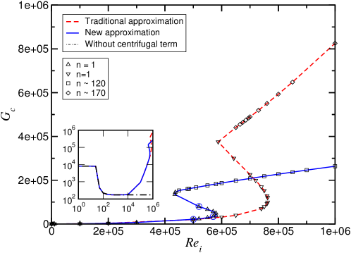
Figure 1: Critical Grashof number $G_{c}$ as function of inner cylinder Reynolds number $\mbox{{Re}}_{i}$ for fluid rotating as a solid-body. The solid line is the linear stability curve using the new approximation for the centrifugal bouyancy proposed in this paper, the dashed corresponds to the traditional Boussinesq approach, whereas the dotted-dashed line is the case without centrifugal buoyancy, which can only be distinguished from the horizontal axis in the inset (log-log axes). Different symbols indicate the two distinct mechanisms of instability. Up and down triangles represent the critical points due to the mechanism at moderate $Re_{i}$ for the new and traditional approximations respectively, whereas squares and diamonds correspond to the mechanism at large $Re_{i}$.

In this case a rotating frame of reference is readily identified and the shear term $B/r$ in the base flow azimuthal velocity (24b) is zero, whereas the term $A$ corresponds to the angular velocity of the cylinders. Figure 1 shows the critical values of $G$ as the rotation speed, indicated here by the inner cylinder Reynolds number $\mbox{{Re}}_{i}$, is increased. In the case of stationary cylinders instability sets in at $G=8087.42$, with $k_{c}=-2.74$ and $n=0$. The emerging pattern is characterized by pairs of counter-rotating torodial rolls, that unlike Taylor vortices have a non-zero phase velocity that causes a slow drift of the cellular pattern upward. Extensive information about natural convection instabilities can be found in the literature: Choi & Korpela (1980) and McFadden et al. (1984) for infinite geometries, and de Vahl Davis & Thomas (1969) and Lee et al. (1982) for finite geometries. Without rotation, traditional (dashed line) and new (solid line) approximations yield identical results to the case where centrifugal buoyancy is neglected (dashed-dotted line). For slow rotation the effect of the centrifugal buoyancy is negligible, and nearly the same critical values are obtained in each case (see inset in figure 1). As rotation is increased, the flow is strongly stabilized by centrifugal bouyancy. Note that if this is neglected, the onset of instability asymptotically approaches $G_{c}=172.50$ and is qualitatively wrong. The presence of the centrifugal term in any of the ways considered here, entirely modifies the stability of the problem and consequently is an essential element to study these flows. No differences between the two approximations in the linear behaviour of the system are observed up to $\mbox{{Re}}_{i}\sim 5\times 10^{5}$, where the two curves start to depart from each other. Up to this point and after a small initial region where several azimuthal modes up to $n=6$ are involved, the base flow loses stability to an azimuthal mode $n=1$ with small axial wavenumber $k\sim 10^{-3}$. The shape of the critical modes along the stability curve is illustrated in figure 2, showing contours of constant temperature in a horizontal cross-section. The three states correspond to the circles in figure 1 and depict the transition between the lower and intermediate branches as we consider the new approximation. As we proceed forward along the critical curve the cold fluid progressively penetrates into the warm fluid and vice versa. The same behaviour is observed when the traditional approximation is used, nevertheless the values of $\mbox{{Re}}_{i}$ and $G_{c}$ required are larger.

$(a)$	$(b)$	$(c)$

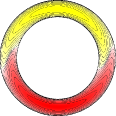
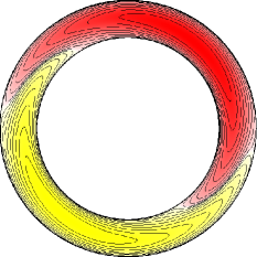
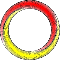
Figure 2: Contours of the temperature disturbance $T^{\prime}$ at a $z$-constant section corresponding to the points marked as blue circles in figure 1. $(a)$: $\mbox{{Re}}_{i}=5\times 10^{5}$, $G_{c}=21206.53$. $(b)$: $\mbox{{Re}}_{i}=5.7\times 10^{5}$, $G_{c}=33768.37$. $(c)$: $\mbox{{Re}}_{i}=5.2\times 10^{5}$, $G_{c}=79670.16$. There are 10 positive (dark gray; red in the online version) and 10 negative (light gray; yellow in the online version) linearly spaced contours. In all cases the critical azimuthal mode is $n=1$ and $k=O(10^{-3})$.

As $\mbox{{Re}}_{i}$ increases beyond $5\times 10^{5}$ the new terms in our approximation start becoming important and lead to different behaviour in the linear stability of the system. An analysis of the magnitude of each term in our approximation reveals that the differences observed in figure 1 at high $\mbox{{Re}}_{i}$ are due to terms involving the product $v_{b}u_{\theta}$, implying the existence of an important centrifugal force acting in azimuthal direction as high rotational speeds are reached. This provides evidence that the traditional formulation, including only the main (radial) contribution of centrifugal buoyancy, is a very good approximation if slow rotation is involved but other contributions may not be neglected in rapidly rotating fluids. Once the critical values given by both approximations differ, we can identify two interesting regions in parameter space. For $\mbox{{Re}}_{i}\in[5\times 10^{5},7.7\times 10^{5}]$ the traditional Boussinesq approach yields larger critical $G$ than our approximation, whereas for $\mbox{{Re}}_{i}>7.7\times 10^{5}$ the upper branch of the new approximation yields much lower critical values. Moreover, the differences keep increasing as $\mbox{{Re}}_{i}$ grows.

$(a)$	$(b)$

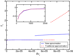
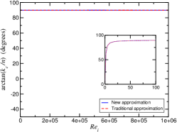
Figure 3: $(a)$ Critical axial wavenumber $k_{c}$ and $(b)$ spiral angle of the modes $\arctan(k_{c}/n)$ as a function of $\mbox{{Re}}_{i}$ for the curves in figure 1. The inset is a close up at low $Re_{i}$ where the first mechanism stops being dominant and is superseded by spiral modes with angle far from $90$ degrees, indeed $0$, corresponding to $n=0$, at $Re_{i}=0$.

The analysis performed reveals the existence of two mechanisms of instability associated with the lower-intermediate and upper branches in figure 1. Different symbols are used to represent the critical values corresponding to each mechanism in each problem. The differences between them are illustrated in figure 3, showing the evolution of the critical axial wavenumber $k_{c}$ and the angle of the spiral modes $\arctan(\frac{k_{c}}{n})$ versus $\mbox{{Re}}_{i}$. Two regions with distinct characteristics are well-defined. The first mechanism of instability has already been presented (see figure 2). Low azimuthal wavenumbers, primarily $n=1$, and very small axial wavenumbers characterize it. This corresponds to quasi two-dimensional modes and can be readily seen in figure 3$(b)$, showing that the angle of the spiral modes remains constant at about $90$ degrees. The inset shows the small initial region where the spiral angle increases progressively until it reaches a vertical position. The second mechanism is characterized by $n>80$ and $k_{c}\sim O(1)$, also corresponding to quasi two-dimensional modes (see figure 3$b$). Another common feature between the two types of instabilities is that the rotational frequency coincides with the angular velocity of the container in both mechanisms and both approximations. This is in agreement with Maretzke et al. (2013), who have analytically proven that two-dimensional modes with $k=0$ always rotate at speed $A$ (24b) in Taylor–Couette flows without heating. An interesting distinct feature of the second instability mechanism is localization near the inner cylinder. An example of these wall convection modes is shown in figure 4; the critical disturbances are clearly different in the traditional and in the new Boussinesq approximations.

$(a)$	$(b)$

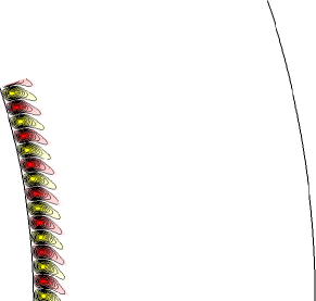
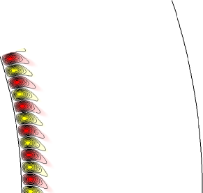
Figure 4: Contours of the critical disturbance temperature on a $z$-constant section for $\mbox{{Re}}_{i}=700000$. $(a)$ Critical mode using the traditional Boussinesq approximation. Here $G_{c}=489371.47$, $k_{c}=1.81$ and $n=150$. $(b)$ Critical mode using the new approximation. Here $G_{c}=207906.92$, $k_{c}=0.54$ and $n=116$. In both cases, only $1/20$ of the domain is shown. There are 10 positive (darker gray; red online) and negative (light gray; yellow online) contours.

6.2 Differentially rotating cylinders

The traditional approximation for the centrifugal buoyancy neglects the part of the base flow containing shear, i.e. the $B/r$ term in (24b). To quantify the influence of including shear in the centrifugal terms, we perform the same analysis as in the previous section but for differentially rotating cylinders. The amount of shear introduced is characterized by the ratio of angular velocities $\beta=\Omega_{i}/\Omega_{o}$; the further $\beta$ is from one, the stronger is the shear effect considered.

6.2.1 Weak shear: rotation close to solid body ($\beta=\Omega_{i}/\Omega_{o}=1.006$)

We first consider the case where the container is rotating near solid body. Although shear may be here expected to play only a secondary role, this case serves the purpose of illustrating the importance of including shear effects in the centrifugal term. Figure 5 shows the neutral stability curve for the two approaches considered and also without centrifugal buoyancy (dashed-dotted line), which produces qualitatively correct results in this instance. Unlike in the solid-body case, the critical values $G_{c}$ increase monotonically as $\mbox{{Re}}_{i}$ grows. Besides shear, centrifugal effects are also important in this configuration. From $\mbox{{Re}}_{i}\gtrsim 2\times 10^{5}$ on the linear stability curves obtained by using both approximations become quite different. Similar features with respect to the solid-body case may be identified. At first the traditional approximation gives lower critical value of the Grashof. However, this region is smaller than in the solid-body case and ends at $\mbox{{Re}}_{i}\sim 2.9\times 10^{5}$ where both curves intersect. From that point on, the stability region predicted by the new approximation is smaller; the differences between the critical values given by both approximations keep increasing as larger $\mbox{{Re}}_{i}$ are considered. At the point where both curves first depart from each other $\mbox{{Re}}_{i}$ has half the value of that of the solid-body case. Consequently, the rotational speeds for which the new approximation is necessary are significantly smaller in the presence of weak differential rotation.

Critical axial and azimuthal wavenumbers exhibit similar behaviour to the solid-body case and so they are not shown here. Two mechanisms of instability are also found. The first one embraces the region $2\times 10^{5}<\mbox{{Re}}_{i}$ and is characterized by $k_{c}\sim 0$ and $1\leq n\leq 6$. Modes are similar to those obtained for the first mechanism in the solid body case. A subtle difference can be nevertheless pointed out. In the solid body situation the temperature disturbances fill the whole annulus, whereas differential rotation confines the perturbation towards the central part (see figure 6$a$). The second mechanism also presents the same features as in the solid body case, high azimuthal modes and $k_{c}\in[0.5,1.5]$, but differences in the flow appear that deserve to be highlighted. In the traditional approximation the dominant wall modes are located at the inner cylinder, as it occurs in the solid-body case (figure 6$b$). In contrast, using the new approximation changes the location of the dominant wall modes to the outer cylinder (figure 6$c$). In view of these results we can say that considering shear effects in the centrifugal term of the Navier–Stokes equations may be extremely important: not only regarding the linear stability boundary but also the shape and location of the critical modes.

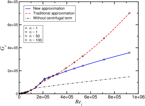
Figure 5: Critical Grashof number $G_{c}$ as function of inner cylinder Reynolds number $Re_{i}$ for rotation near solid-body ($\beta=1.006$). Different symbols refer to two distinct instability mechanisms as in figure 1.

$(a)$	$(b)$	$(c)$

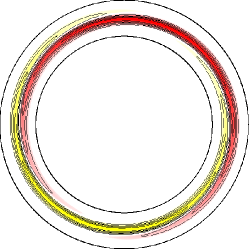
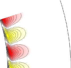
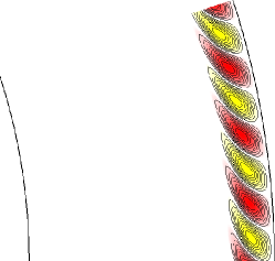
Figure 6: Contours of the critical disturbance temperature on a $z$-constant section. $(a)$ $n=1$, $\mbox{{Re}}_{i}=178125$, $G_{c}=92987.56$. $(b)$–$(c)$ Comparison of the traditional $(b)$ and new $(c)$ approximation at $\mbox{{Re}}_{i}=285000$ (near the crossover point in figure 5) showing $1/20$ of the annulus. $(b)$ $G_{c}=154864.79$, $k_{c}=0.24$ and $n=30$. $(c)$ $G_{c}=156547.54$, $k_{c}=0.39$ and $n=75$. There are ten positive (dark gray; red online) and negative (light gray; yellow online) linearly spaced contours.

6.2.2 Strong shear: Quasi-Keplerian rotation ($\beta=\Omega_{i}/\Omega_{o}=1.58$)

If $1/\eta>\beta>1$ the angular velocity decreases outward but the angular momentum increases. These flows, known as quasi-Keplerian flows, are used as models to investigate the dynamics and stability of astrophysical accretion disks. Here we choose a typical value $\beta=1.58$ and as in the previous sections consider a negative temperature gradient in the radial direction, as expected in accretion disks. Figure 7 shows the neutral stability curve for the two approximations considered, as well as entirely neglecting centrifugal effects ($\epsilon=0$). The three curves are almost straight lines, that completely overlap in a plot $(G_{c},Re_{i})$. In order to see the small differences that appear at large $Re_{i}$, we have plotted in this case $G_{c}/Re_{i}$ versus $Re_{i}$. Shear is the completely dominant mechanism in this regime, but small differences can be observed for $Re_{i}\gtrsim 2\times 10^{5}$, that are enhanced in the inset. Surprisingly, shear has a very strong stabilizing effect in this problem: without shear the critical Grashof number is ten times smaller at $Re_{i}=10^{6}$ than in the quasi-Keplerian case.

Depending on the Reynolds number two mechanisms of instability are again found. The first mechanism exhibits a similar flow structure to that observed in the previous case. It also occurs at low $\mbox{{Re}}_{i}$ and is localized in the central part of the annulus due to the action of differential rotation. Figure 8$(a)$ shows the contours of the disturbance temperature in an horizontal plane. In contrast to what happens in the weak shear situation, these modes present a clear 3D structure with $k_{c}\sim-1$. Small azimuthal wavenumbers are involved in this mechanism, ranging from $n=1$ to $n=6$. More remarkable differences are found when analysing the second mechanism. High azimuthal modes $n\sim 50$ arise as this mechanism becomes dominant, but unlike the solid-body and weak shear situations, the azimuthal mode number decreases as $\mbox{{Re}}_{i}$ increases. The same behaviour is observed in the axial wavenumber, so that the spiral angle quickly converges to $90$ degrees as observed in the previous sections. Figure 8$(b)$ shows that the instability is characterized by convection wall modes localized at the outer cylinder, as in the case of weak shear using the new approximation. Nevertheless, in quasi-Keplerian flows the dominant modes are always localized at the outer cylinder regardless of how centrifugal terms enter the equations.

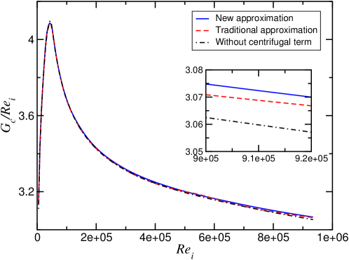
Figure 7: Critical ratio $G_{c}/Re_{i}$ as function of inner cylinder Reynolds number $Re_{i}$ for quasi-Keplerian rotation ($\beta=1.58$). The three curves differ only by about 1% and hence are only distinguishable in the inset.

$(a)$	$(b)$

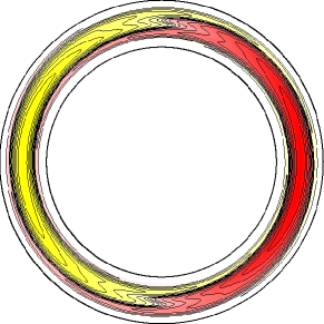
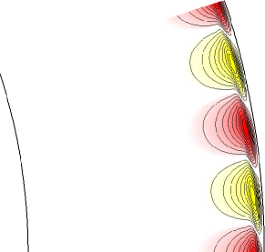
Figure 8: Contours of the critical disturbance temperature on a $z$-constant section. $(a)$ $\mbox{{Re}}_{i}=11681.03$ with $G_{c}=4.1268\times 10^{4}$, $k_{c}=-1.05$ and $n=1$. $(b)$ $\mbox{{Re}}_{i}=584051.72$ with $G_{c}=1.8511\times 10^{4}$, $k_{c}=8.21$ and $n=38$. Ten positive (dark gray; red online) and negative contours (light gray; yellow online) are displayed. Only $1/20$ of the domain is shown in $(b)$.

7 Summary and discussion

We have identified weaknesses in how the Boussinesq formulation is typically used to account for centrifugal buoyancy in the Navier–Stokes equations. In particular, the traditional approximation (including only the term $\rho^{\prime}\Omega^{2}$) neglects the effects associated with differential rotation or strong internal vorticity. This has motivated us to develop a new consistent Boussinesq-type approximation correcting this problem. It consists in keeping the density variations in the advection term of the Navier-Stokes equations and thus it is very easy to implement in an existent solver. The new approximation allows accurate treatment of situations with differential rotation or when strong vortices appear in the interior of the domain, which may cause important centrifugal effects even in flows without global rotation. The latter may be especially relevant in simulations at high Rayleigh numbers (as e.g. in the quest for the ‘ultimate regime’, Ahlers et al., 2009). Thus we argue that our formulation for the centrifugal terms should be always implemented whenever the Boussinesq approximation is used.

The relevance of the new approximation has been illustrated with a linear stability analysis of a Taylor–Couette system subjected to a negative radial gradient of temperature. Three different cases have been studied. First, we have considered the container rotating as solid-body, i.e. without differential rotation. We note that if centrifugal buoyancy is entirely neglected, the results are even qualitatively wrong. For both traditional and new approximations the critical values obtained agree up to $\mbox{{Re}}_{i}\sim 5.5\times 10^{5}$, beyond which discrepancies become significant. Beyond this point the conductive base flow loses stability to quasi two-dimensional wall modes (aligned with the axis of rotation, as expected from the Taylor–Proudman Theorem) localized at the inner cylinder. Note that the large discrepancy in critical Grashof numbers observed at $\mbox{{Re}}_{i}\in[5\times 10^{5},10^{6}]$ between both approximations makes it possible to test them against laboratory experiments. For example, in the experiments from Paoletti & Lathrop (2011), and Avila & Hof (2013), which allow for radial temperature gradients, $\mbox{{Re}}=10^{6}$ can be reached, and the required Grashof numbers $5\times 10^{5}$ can be obtained with temperature differences about half a degree kelvin.

We have also considered the case in which the cylinders rotate at different angular speeds, thus introducing shear. For weak differential rotation, shear and centrifugal buoyancy effects compete and the critical values obtained with both approximations differ from each other at lower $\mbox{{Re}}_{i}\sim 2\times 10^{5}$. Moreover, the new approximation gives rise to wall modes located on the outer cylinder, whereas the traditional approach yields wall modes on the inner cylinder, as in the solid-body case. In quasi-Keplerian flows, shear is so dominant that centrifugal terms may be entirely neglected in the linear stability analysis (discrepancies in $G_{c}$ are below 1% regardless of how centrifugal terms enter the equations, if at all). Here the critical modes are always localized at the outer cylinder. Note that such wall modes, similar to those identified by Klahr et al. (1999), are not relevant to the accretion disk problem, in which there are no solid radial boundaries. Furthermore, it is worth noting that testing our differential rotation results in the laboratory is very difficult because of axial endwall effects. The large Re involved will necessarily trigger instabilities and transition to turbulence because of the nearly discontinuous angular velocity profile at the junction between axial endwalls and cylinders (Avila, 2012).

Although it may be tempting to suggest that laminar quasi-Keplerian flows are stable for weak stratification in the radial direction, our analysis has only axial gravity, and is linear and hence concerned with infinitesimal disturbances only. In more realistic models of accretion disks, nonlinear baroclinic instabilities have been found in similar regimes by Klahr & Bodenheimer (2003), and we expect that subcritical transition via finite amplitude disturbances may occur in the problem investigated here. This remains a key question for incoming numerical and experimental investigations. In fact, even in the classical (isothermal) Taylor–Couette problem this possibility remains open and controversial (see e.g. Balbus, 2011).