Gluon mass generation in the presence of dynamical quarks

Abstract

We study in detail the impact of dynamical quarks on the gluon mass generation mechanism, in the Landau gauge, for the case of a small number of quark families. As in earlier considerations, we assume that the main bulk of the unquenching corrections to the gluon propagator originates from the fully dressed quark-loop diagram. The nonperturbative evaluation of this diagram provides the key relation that expresses the unquenched gluon propagator as a deviation from its quenched counterpart. This relation is subsequently coupled to the integral equation that controls the momentum evolution of the effective gluon mass, which contains a single adjustable parameter; this constitutes a major improvement compared to the analysis presented in Phys. Rev. D86 (2012) 014032, where the behaviour of the gluon propagator in the deep infrared was estimated through numerical extrapolation. The resulting nonlinear system is then treated numerically, yielding unique solutions for the modified gluon mass and the quenched gluon propagator, which fully confirm the picture put forth recently in several continuum and lattice studies. In particular, an infrared finite gluon propagator emerges, whose saturation point is considerably suppressed, due to a corresponding increase in the value of the gluon mass. This characteristic feature becomes more pronounced as the number of active quark families increases, and can be deduced from the infrared structure of the kernel entering in the gluon mass equation.

I Introduction

The concept of a momentum-dependent gluon mass Cornwall (1982) has been the focal point of considerable attention in recent years, mainly because it offers a natural and self-consistent explanation Aguilar et al. (2008) for the infrared finiteness of the (Landau gauge) gluon propagator and ghost dressing function, observed in large-volume lattice simulations, both in $SU(2)$ Cucchieri and Mendes (2007) and in $SU(3)$ Bogolubsky et al. (2009). Given the purely nonperturbative nature of the associated mass generation mechanism, the Schwinger-Dyson equations (SDEs) constitute the most appropriate framework for studying such phenomenon in the continuum Binosi and Papavassiliou (2008a); Alkofer and von Smekal (2001); Fischer (2006); Braun et al. (2010).

At the level of the SDEs, the general analysis finally boils down to the study of an integral equation, to be referred as the mass equation Aguilar et al. (2011); Binosi et al. (2012), which governs the evolution of the dynamical gluon mass, $m^{2}(q^{2})$, as a function of the momentum $q^{2}$ (see Eq. (7) below). It turns out that this special equation has been derived exactly, following the elaborate procedure explained in detail in Binosi et al. (2012). This particular construction was carried out within the framework provided by the synthesis of the pinch technique (PT) Cornwall (1982); Cornwall and Papavassiliou (1989); Pilaftsis (1997); Binosi and Papavassiliou (2002a); Binosi and Papavassiliou (2004, 2009) with the background field method (BFM) Abbott (1981), known in the literature as the PT-BFM scheme Aguilar and Papavassiliou (2006); Binosi and Papavassiliou (2008a, b).

This exact mass equation, however, may not be treated in its complete form, because a particular field-theoretic ingredient entering in it is not fully known. Therefore, an approximate version of the full equation has been considered instead Binosi et al. (2012), which depends on a free adjustable parameter. The detailed numerical study of this particular equation, for pure $SU(3)$ Yang-Mills, revealed that its solutions depend strongly on the precise shape of the gluon propagators entering in its kernel. In particular, the $q^{2}$ region below 1 GeV² appears to be crucial for obtaining physically acceptable (i.e., positive-definite and monotonically decreasing) solutions.

Interestingly enough, as has been shown in recent SDEs Aguilar et al. (2012a) and lattice studies Ayala et al. (2012), the gluon propagator, $\Delta(q^{2})$, undergoes considerable changes in this particular region of momenta when a small number of light (dynamical) quarks is included in the theory, i.e., when “unquenching” takes place. This basic observation, in turn, motivates the further scrutiny of the mass equation under the special conditions that occur when the transition from pure Yang-Mills to real world QCD takes place. In particular, it is clearly of the outmost importance to establish, in quantitative detail, how the inclusion of dynamical quarks affects the entire mechanism of gluon mass generation. In fact, from the point of view of computing unquenching effects to the gluon propagator, the present work constitutes a sequel to Aguilar et al. (2012a), whose main improvement is the incorporation of the gluon mass equation into the general dynamical analysis (in the context of the so-called “scaling” solutions, where no mass scale is generated, the unquenching effects have been investigated in detail in Fischer and Alkofer (2003); Fischer et al. (2005)).

If one subscribes to the interpretation that the infrared finiteness of the lattice propagators is a consequence of the generation of such a mass, then the new unquenched lattice results of Ayala et al. (2012) would seem to indicate that the general mass generation picture persists in the presence of quark loops. In fact, the observed considerable suppression of the value of the saturation point of the unquenched propagators with respect to the quenched ones, would clearly suggest that the corresponding gluon mass increases [since $\Delta^{-1}(0)=m^{2}(0)]$. To be sure, this basic argument must be supplemented by a more careful analysis, taking into account the effects of renormalization. In particular, the required renormalization of the gluon propagators by a multiplicative constant may shift the location of their corresponding saturation points. However, provided that all curves are renormalized at the same (subtraction) point, the relative size (ratio) between these saturation points will remain unaltered, indicating the aforementioned relative increase of the effective gluon mass.

To explore this fundamental issue systematically, one needs a faithful description of the effects of the inclusion of quark-loops to the gluon propagator. To be sure, one could envisage the possibility of substituting the unquenched lattice data directly into the mass equation, in a spirit similar to that followed in the pure Yang-Mills case. However, we will refrain from using this latter set of data, and will resort instead to the full SDE approach presented in Aguilar et al. (2012a), which allows the approximate inclusion of such effects in the quenched propagator.

This particular approach assumes the presence of a small number of quark families, and treats the entire effect of “unquenching” as a “perturbation” to the quenched gluon propagator. Then, the main bulk of the “unquenching” is attributed to the fully dressed quark-loop graph, while higher loop contributions are considered to be subleading. The inclusion of this particular nonperturbative loop induces considerable modifications to the shape of the resulting propagator, but does not provide precise information on the existence and value of the new saturation point. Indeed, such information may be only gathered in conjunction with the gluon mass equation, which was unavailable at the time of the original analysis. As a result, in the work of Aguilar et al. (2012a) the existence of a saturation point was assumed, and its approximate value was obtained through simple extrapolation from the overall shape of the propagator in the region around 0.05 GeV².

Here, instead, our present knowledge of the mass equation allows us to carry out a thorough analysis of this particular dynamical question. Specifically, the equation describing the unquenching of the gluon propagator is coupled to the mass equation, and the resulting non-linear system is solved numerically. In this way, one eventually obtains as a result the unquenched gluon propagator in the entire range of physically relevant momenta, including the value of its saturation point.

The main result of this article may be summarized as follows. The solution of the system reveals that the mass equation yields physical solutions in the presence of quarks, specifically for the typical cases $N_{\!f}=2$ (two degenerate light quarks), and $N_{\!f}=2+1+1$ (two degenerate light quarks and two heavy ones), considered in the recent lattice simulations Ayala et al. (2012). In fact, one establishes clearly that the value of the gluon mass at the origin increases as additional quarks are included in the theory. In addition, one obtains a concrete prediction for the quenched gluon propagator, which compares rather favorably with the aforementioned lattice results. We emphasize that throughout this analysis we make use of a single adjustable parameter, which is meant to model contributions to the mass equations stemming from the fully-dressed three gluon vertex.

The article is organized as follows. In Section II, we first define the basic quantities appearing in the problem, and introduce some important relations characteristic to the PT-BFM framework. Then, we describe the modifications that must be implemented at the level of the gluon SDE in order to consistently accommodate a dynamical gluon mass. Finally, we review the theoretical origin and properties of the two key dynamical equations, namely the gluon mass (integral) equation and the unquenching formula. Section III is dedicated to the solution of the system formed when the aforementioned two equations are coupled to each other. To that end, we begin by reviewing the main ingredients appearing in them, and spell out the approximations employed in their treatment. Then we proceed to the numerical solution, describing in detail the iterative procedure adopted. The numerical results obtained are then compared with the latest lattice results, and some of the possible reasons for the observed deviations are discussed. Our conclusions are finally presented in Section IV.

II Gluon Mass equation with unquenched gluon propagators

The full gluon propagator (quenched or unquenched) in the Landau gauge assumes the general form

$$i{\Delta}_{\mu\nu}(q)=-i{\Delta}(q^{2})P_{\mu\nu}(q);\qquad P_{\mu\nu}(q)=g_{\mu\nu}-{q_{\mu}q_{\nu}}/{q^{2}},$$ (1)

where $\Delta(q^{2})$ is related to the scalar form factor of the gluon self-energy $\Pi_{\mu\nu}(q)=\Pi(q^{2})P_{\mu\nu}(q)$ through

$$\Delta^{-1}(q^{2})=q^{2}+i\Pi(q^{2})\,.$$ (2)

In addition, the corresponding inverse gluon dressing function, $J(q^{2})$, is defined as

$$\Delta^{-1}(q^{2})=q^{2}J(q^{2}),$$ (3)

and, as has been explained in Aguilar and Papavassiliou (2010); Aguilar et al. (2011), it is intimately related with the definition of the renormalization-group invariant QCD effective charge.

As has been demonstrated in detail in the recent literature Aguilar et al. (2012b); Ibanez and Papavassiliou (2012), the nonperturbative dynamics of Yang-Mills theories gives rise to a dynamical (momentum-dependent) gluon mass, which accounts for the infrared finiteness of $\Delta(q^{2})$. Specifically, from the kinematic point of view, we will describe the transition from a massless to a massive gluon propagator by carrying out the replacement $\Delta^{-1}(q^{2})\to\Delta_{m}^{-1}(q^{2})$, where (Minkowski space)

$$\Delta_{m}^{-1}(q^{2})=q^{2}J_{m}(q^{2})-m^{2}(q^{2}).$$ (4)

Notice that the subscript “$m$” indicates that effectively one has now a mass inside the corresponding expressions: for example, whereas perturbatively $J(q^{2})\sim\ln q^{2}$, after dynamical gluon mass generation has taken place, one has $J_{m}(q^{2})\sim\ln(q^{2}+m^{2})$. The presence of this mass, in turn, tames the Landau pole appearing in the (perturbative) effective charge, causing its saturation in the deep infrared Aguilar et al. (2009a); Aguilar et al. (2010).

From the dynamical point of view, the emergence of massive solutions from the gluon propagator SDE depends crucially on the inclusion of a set of special vertices, to be generically denoted by $V$ and called pole vertices Aguilar et al. (2011), which contain massless, longitudinally coupled poles. These vertices are added to the usual (fully dressed) vertices of the theory, and have a two-fold effect: they trigger the well-known Schwinger mechanism, thus endowing the gluon with a dynamical mass, while, at the same time, they guarantee that the Slavnov-Taylor identities (STIs) of the theory maintain exactly the same form before and after the mass has been dynamically generated. In particular, the transversality of $\Pi_{\mu\nu}(q)$ in the presence of masses is preserved, provided that one replaces all vertices $\Gamma$ appearing in the gluon SDE by

$$\Gamma\longrightarrow\Gamma^{\prime}=\Gamma_{m}+V,$$ (5)

with $V$ having the precise structure that will make the new vertices $\Gamma^{\prime}$ satisfy the same formal STIs as the $\Gamma$ before, but with the replacement $\Delta^{-1}\longrightarrow\Delta_{m}^{-1}$.

It turns out that $J_{m}(q^{2})$ and $m^{2}(q^{2})$ satisfy two separate, but coupled, integral equations of the generic type Aguilar et al. (2011)

$$J_{m}(q^{2})=1+\int_{k}{\cal K}_{1}(k,q,m^{2},\Delta),$$

$$m^{2}(q^{2})=\int_{k}{\cal K}_{2}(k,q,m^{2},\Delta),$$ (6)

such that ${\cal K}_{1},{\cal K}_{2}\neq 0$, as $q\rightarrow 0$. In the equations above we have introduced the dimensional regularization measure $\int_{k}=\mu^{\epsilon}\int\!{\rm d}^{d}k/(2\pi)^{d}$ where $d=4-\epsilon$ is the space-time dimension and $\mu$ the ’t Hooft mass.

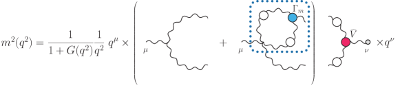
Figure 1: The effective SDE satisfied by the dynamical gluon mass. The blue vertex corresponds to the vertex $\Gamma_{m}$ of Eq. (5), while the red vertex $\widetilde{V}$ indicates a pole vertex in which one of the gluon is leg is a background leg. Finally, the box singles out the quantity $Y(k^{2})$ which represents the purely two-loop dressed correction to the one-loop dressed mass equation kernel.

The exact closed form of the kernel ${\cal K}_{2}$, and hence the full integral equation that determines $m^{2}(q^{2})$, has been derived in Binosi et al. (2012), by appealing to the special properties of the pole vertices $V$. The resulting homogeneous equation is given by Binosi et al. (2012) (see also Fig. 1)

$$m^{2}(q^{2})=-\frac{g^{2}C_{A}}{1+G(q^{2})}\frac{1}{q^{2}}\int_{k}m^{2}(k^{2})\Delta_{\rho}^{\mu}(k)\Delta^{\nu\rho}(k+q){\cal K}_{\mu\nu}(k,q),$$ (7)

with

$${\cal K}_{\mu\nu}(k,q) = [(k+q)^{2}-k^{2}]\left\{1-[Y(k+q)+Y(k)]\right\}g_{\mu\nu}$$ (8)

$$+ [Y(k+q)-Y(k)](q^{2}g_{\mu\nu}-2q_{\mu}q_{\nu}).$$

The quantity $Y$ represents the subdiagram nested inside the two-loop dressed graph of Fig. 1, given by

$$Y(k^{2})=\frac{g^{2}C_{A}}{4k^{2}}\,k_{\alpha}\!\int_{\ell}\!\Delta^{\alpha\rho}(\ell)\Delta^{\beta\sigma}(\ell+k)\Gamma_{\sigma\rho\beta}(-\ell-k,\ell,k),$$ (9)

with $\Gamma_{\sigma\rho\beta}$ the full three-gluon vertex, and $C_{A}$ the Casimir eigenvalue in the adjoint representation [$C_{A}=N$ for $SU(N)$].

Finally, the function $G(q^{2})$ corresponds to the $g_{\mu\nu}$ component of a special two point-function, which constitutes a crucial ingredient in a set of powerful identities, relating the conventional Green’s functions to those of the BFM Grassi et al. (2001); Binosi and Papavassiliou (2002b). For the case of the conventional gluon propagator, $\Delta$, and the PT-BFM gluon propagator, denoted by $\widehat{\Delta}$, the relevant identity reads

$$\Delta(q^{2})=[1+G(q^{2})]^{2}\widehat{\Delta}(q^{2});$$ (10)

its application at the level of the corresponding SDEs leads to the appearance of the factor $1+G(q^{2})$ in Eq. (7).

The numerical treatment of Eq. (7), under certain simplifying assumptions regarding the form of $Y(k^{2})$ (see next section), gave rise to solutions that display the basic qualitative features expected on general field-theoretic considerations, and employed in numerous phenomenological studies. In particular, the $m^{2}(q^{2})$ obtained are monotonically decreasing functions of the momentum and vanish rather rapidly in the ultraviolet Cornwall (1982); Binosi et al. (2012).

As explained in the Introduction, the purpose of the present work is to study the effects induced on the gluon mass by the inclusion of a small number of light quark families. To that end, one needs to solve Eq. (7) using unquenched gluon propagators, $\Delta_{\scriptscriptstyle N_{\!f}}(q^{2})$, namely carrying out the substitution $\Delta(q^{2})\to\Delta_{\scriptscriptstyle N_{\!f}}(q^{2})$ inside the integral of the r.h.s..

The corresponding expression for $\Delta_{\scriptscriptstyle N_{\!f}}(q^{2})$ will be obtained following the SDE approach presented in Aguilar et al. (2012a). Specifically, one assumes that the main bulk of the unquenching effect is captured by the (fully dressed) one-loop diagram of Fig. 2 (b), neglecting, at this level of approximation, all contributions stemming from (higher order) diagrams containing nested quark loops.

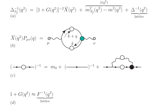
Figure 2: Schematic representation of the unquenched propagator $(a)$, corresponding to Eq. (15), and some of the ingredients [$(b)$, $(c)$, and $(d)$] entering in it. In particular, $(b)$ represents the quark loop, which, in the approximation employed, is the only source of quark-dependence. The quark propagators entering in $(b)$ are solutions of the gap equation depicted in $(c)$, where $m_{0}$ denotes the appropriate current mass. Finally, the function $G(q^{2})$ is obtained from the relation shown in $(d)$, namely Eq. (18). The quantities obtained from the lattice are also indicated. Note that the term $\lambda^{2}(q^{2})$ will be determined dynamically, once the mass equation of Fig. 1 is coupled to $(a)$.

Denoting the contribution of this special diagram by

$$\widehat{X}_{\mu\nu}(q)=\widehat{X}(q^{2})P_{\mu\nu}(q),$$ (11)

we have that

$$\widehat{X}(q^{2})=-\frac{g^{2}}{6}\!\int_{k}\mathrm{Tr}\left[\gamma^{\mu}S(k)\widehat{\Gamma}_{\mu}(k,-k-q,q)S(k+q)\right].$$ (12)

where $S$ denotes the full quark propagator, and the vertex $\widehat{\Gamma}_{\mu}$ corresponds to the PT-BFM quark-gluon vertex, satisfying the QED-like Ward identity

$$iq^{\mu}\widehat{\Gamma}_{\mu}(k,-k-q,q)=S^{-1}(k)-S^{-1}(k+q).$$ (13)

Of course, in the case of including various quark loops, corresponding to different quark flavors $N_{\!f}$, the term $\widehat{X}^{\mu\nu}(q)$ in Eq. (11) is replaced simply by the sum over all quark loops, i.e.,

$$\widehat{X}^{\mu\nu}(q)\to\sum_{f}\widehat{X}_{f}^{\mu\nu}(q).$$ (14)

Then, the detailed analysis of Aguilar et al. (2012a) reveals that the unquenched gluon propagator $\Delta_{\scriptscriptstyle N_{\!f}}(q^{2})$ may be expressed as a deviation from the quenched propagator $\Delta(q^{2})$, namely (Euclidean space)

$$\Delta_{\scriptscriptstyle N_{\!f}}(q^{2})=\frac{\Delta(q^{2})}{1+\left\{\widehat{X}(q^{2})\left[1+G(q^{2})\right]^{-2}+\lambda^{2}(q^{2})\right\}\Delta(q^{2})},$$ (15)

where the quantity

$$\lambda^{2}(q^{2})=m^{2}_{\scriptscriptstyle N_{\!f}}(q^{2})-m^{2}(q^{2}),$$ (16)

measures the difference induced to the gluon mass due to the inclusion of quarks.

An important point, which can be established formally and confirmed numerically Aguilar et al. (2012a), is that the nonperturbative $\widehat{X}(q^{2})$ vanishes at the origin, $\widehat{X}(0)=0$, exactly as it happens in perturbation theory. This implies that the mass equation is not directly affected by the presence of dynamical quarks, as the methodology used to derive Eqs. (7), (8) and (9) is left invariant by the unquenching procedure. However, the solutions of the corresponding equation will be different from those obtained in the quenched case, as the kernel ${\cal K}_{\mu\nu}$ will change, due to the modifications induced by $\widehat{X}(q^{2})$ in the overall shape of the propagator throughout the entire range of momenta. Thus, the inclusion of quark loops affects the value of the saturation point of the gluon propagator, not directly through the presence of the $\widehat{X}(q^{2})$, rather indirectly through the generation of a non vanishing mass difference $\lambda^{2}(q^{2})$.

The next nontrivial step is therefore to treat the mass equation Eq. (7) and the unquenching master formula of Eq. (15) as a coupled system, and determine both $m^{2}_{\scriptscriptstyle N_{\!f}}$ and $\Delta_{\scriptscriptstyle N_{\!f}}(q^{2})$. This rather involved task will be undertaken in detail in the next section.

III Numerical analysis

Before entering into the technical details of the solution of the system, it is important to comment on a fundamental qualitative difference between the present situation and the treatment followed in Binosi et al. (2012). Specifically, as already explained in the previous section, even in the absence of quarks, Eq. (7) forms part of a system of coupled equations, namely that of Eq. (6). However, given that the corresponding equation for $J_{m}(q^{2})$ is only partially known, the approach adopted in Binosi et al. (2012) was to treat the gluon propagators appearing in Eq. (6) as external quantities, using the lattice results of Bogolubsky et al. (2009) for their functional form. As a consequence, the intrinsically non-linear equation (6) (recall Eq. (4)) was converted into a linear one. As a result of this linearity, one obtained a continuous family of solutions, parametrized by the values of a multiplicative constant; the actual solution chosen was the one that reproduced the saturation point of the lattice gluon propagator that was used as input in Eq. (6).

Here, instead, even though we still decouple the equation for $J_{m}(q^{2})$, the mass equation retains its non-linear nature due to the form of the unquenched gluon propagator, $\Delta_{\scriptscriptstyle N_{\!f}}(q^{2})$, that will be inserted in it. Specifically, as can be appreciated from Eq. (15), the $\lambda^{2}(q^{2})$ appearing in the denominator of $\Delta_{\scriptscriptstyle N_{\!f}}(q^{2})$ introduces a non-linear term into Eq. (6). Consequently, the solution obtained will be unique, and the saturation point of the resulting $\Delta_{\scriptscriptstyle N_{\!f}}(q^{2})$ will emerge as a prediction of the theory rather than as an input from the lattice.

III.1 Main ingredients and basic assumptions

We next proceed to a brief description of the ingredients entering into the two equations (6) and (15) composing the system under study, together with an account of the most important underlying assumptions.

(i ) The determination of the quantity $\widehat{X}(q^{2})$ is of central importance, since it approximates the entire effect of the inclusion of the active quarks. In order to evaluate it from Eq. (12), one needs specific expressions for the full quark propagator $S$ and the fully-dressed vertex $\widehat{\Gamma}$. Evidently, the total $\widehat{X}(q^{2})$ emerges as the sum of the individual flavor contributions, in accordance with Eq. (14).

The nonperturbative form of each quark propagator entering into $\widehat{X}(q^{2})$ is obtained from the standard gap equation Aguilar and Papavassiliou (2011), supplemented by an appropriate current mass term, in order to make contact with the lattice results of Ayala et al. (2012). In this latter simulation, the gluon (and ghost) propagators have been evaluated from large volume configurations (up to $3^{3}\times 6$ [fm⁴]), generated from a lattice action that included (twisted mass) fermions. Specifically, one employed two light degenerate quarks ($N_{\!f}=2$), with a current mass ranging from 20 to 50 MeV, or two light and two heavy quarks ($N_{\!f}=2+1+1$), with a strange (charm) quark current mass roughly set to 95 MeV (1.51 GeV).

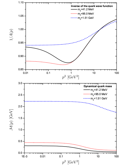
Figure 3: (color online) The inverse of the quark wave-functions (top), and dynamical quark masses (bottom), obtained from the quark gap equation for three different values of the current mass: $m_{0}=41.2$ MeV (black, continuous), $m_{0}=95$ MeV (red, dotted) and $m_{0}=1.51$ GeV (blue, dashed).

For the quark propagator, $S(p)$, we use the standard parametrization

$$S^{-1}(p)=-i\left[A(p)p/-B(p)\right]=-iA(p)\left[p/-{\cal M}(p)\right],$$ (17)

where $A(p)$ represents the “quark wave-function”, while the ratio ${\cal M}(p)=B(p)/A(p)$ denotes the dynamical quark mass, and extracts them from the corresponding system of integral equations. The inverse of the quark wave-functions, $1/A(p)$, and the dynamical quark masses, ${\mathcal{M}}(p)$, used in the present work, are shown in the top and bottom panels of Fig. 3, respectively. They have been obtained from the gap equation of Aguilar and Papavassiliou (2011), where the quenched lattice data of Bogolubsky et al. (2009) were used as input.

As can be seen from Fig. 3 the two degenerate light quarks acquire a physical mass around $300$ MeV, while the two heavier ones get physical masses around 440 MeV (strange) and 2.2 GeV (charm). It should be stressed that these values for the quark masses are consistent with the ones generally employed in phenomenological calculations Maris and Roberts (2003); Wilson et al. (2012).

As for the PT-BFM quark-gluon vertex $\widehat{\Gamma}$, the fact that it satisfies the Abelian Ward identity of Eq. (13) allows one to model it by means of the standard Abelian Ansätze existing in the literature Ball and Chiu (1980); Curtis and Pennington (1990). In particular, $\widehat{\Gamma}$ is expressed entirely in terms of the quantities $A(p)$ and ${\cal M}(p)$, with no reference to auxiliary ghost Green’s functions, a fact that simplifies considerably the task of computing $\widehat{X}(q^{2})$.

When all the aforementioned ingredients are put together, the two different $\widehat{X}(q^{2})$, corresponding to the cases $N_{\!f}=2$ (black, continuous) and $N_{\!f}=2+1+1$ (blue, dashed), are shown in Fig. 4.

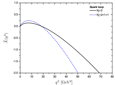
Figure 4: The full nonperturbative quark loop contribution $\widehat{X}(q^{2})$ for the two cases $N_{\!f}=2$ (black, continuous) and $N_{\!f}=2+1+1$ (blue, dashed).

Note finally that, as one can establish formally and confirm numerically Aguilar et al. (2012a), the nonperturbative $\widehat{X}(q^{2})$ vanishes at the origin, $\widehat{X}(0)=0$, exactly as it happens in perturbation theory. Evidently, the inclusion of quark loops does not affect directly the value of the saturation point of the gluon propagator. However, as already explained, the saturation point will be indirectly affected, due to the modifications induced by $\widehat{X}(q^{2})$ in the overall shape of the propagator, throughout the entire range of momenta.

Figure 5: The curves formed by the set of the pairs $(C\alpha_{s},\alpha_{s})$ yielding physical solutions to the full mass equation (7), for the various numbers of quark families $N_{\!f}$: quenched (red, dots), $N_{\!f}=2$ (green, triangles) and $N_{\!f}=2+1+1$ (blue, squared). At the values of $C$ indicated by the stars, the solutions obtained corresponds to the expected values of the strong coupling $\alpha_{s}$ at the scale chosen ($\mu=4.3$ GeV); one has $C=9.04$ for $N_{\!f}=0$ ($\alpha_{s}=0.22$), $C=8.48$ for $N_{\!f}=2$ ($\alpha_{s}=0.285$), and $C=8.64$ for $N_{\!f}=2+1+1$ ($\alpha_{s}=0.33$). Finally, the values of $\alpha_{s}$ obtained for the case in which $Y$ is simply kept at the lowest order perturbative value (i.e., $C=1$) are $\alpha_{s}=0.93$ ($N_{\!f}=0$), $\alpha_{s}=1.09$ ($N_{\!f}=2$), and $\alpha_{s}=1.25$ ($N_{\!f}=2+1+1$).

(ii ) As already mentioned, the quenched lattice data for $\Delta(q^{2})$ Bogolubsky et al. (2009) constitute the starting point for obtaining from Eq. (15) a prediction for $\Delta_{\scriptscriptstyle N_{\!f}}(q^{2})$. In addition, in the Landau gauge, the quantity $1+G(q^{2})$, appearing in both Eqs. (6) and (15), is linked to the inverse of the ghost dressing function $F(q^{2})$ through Grassi et al. (2004); Aguilar et al. (2009b)

$$F^{-1}(q^{2})\approx 1+G(q^{2}).$$ (18)

This relation, which is valid to a very good approximation, and becomes an exact equality at $q^{2}=0$, allows one to use the lattice results of Bogolubsky et al. (2009) for the ghost dressing function, in order to determine $G(q^{2})$. Notice that both sets of data will be renormalized at the scale $\mu=4.3$ GeV, which is the last available point in the ultraviolet. At this scale, the expected value of the (quenched) strong effective charge is $\alpha_{s}=g^{2}/4\pi=0.22$ Boucaud et al. (2006, 2009).

(iii ) The function $Y(k^{2})$ represents a crucial ingredient of Eq. (7). However, its exact closed form is not available, mainly because our present knowledge of the full three-gluon vertex, entering in its definition, is relatively limited; we must therefore resort to suitable approximations. In particular, we will employ the lowest-order perturbative expression for $Y(k^{2})$, obtained from Eq. (9) by substituting the tree-level values for all quantities appearing there. Within this approximation, and after carrying out momentum subtraction renormalization (MOM) at $k^{2}=\mu^{2}$, one obtains Binosi et al. (2012)

$$Y_{\mathrm{R}}(k^{2})=-\frac{\alpha_{s}C_{A}}{4\pi}\frac{15}{16}\log\frac{k^{2}}{\mu^{2}},$$ (19)

where $\alpha_{s}$ is the value of the coupling at the subtraction point chosen. This simple approximation will be compensated, in part, by multiplying $Y_{\mathrm{R}}(k^{2})$ by and arbitrary constant $C$, i.e., by implementing the replacement $Y_{\mathrm{R}}(k^{2})\to C\,Y_{\mathrm{R}}(k^{2})$ treating $C$ as a free parameter. In this heuristic way, one hopes to model further corrections that may be added to the “skeleton” result provided by Eq. (19). This particular procedure has been proved sufficient for obtaining in the quenched case physically meaningful solutions for $m^{2}(q^{2})$ for reasonable values of the constant $C$ Binosi et al. (2012). As the numerical study presented in Fig. 5 shows, this continues to be true also in the unquenched case.

(iv ) A particularly helpful constraint may be obtained by taking the $q^{2}\to 0$ limit of the mass equation (7), which gives (passing to spherical coordinates, and setting $y=k^{2}$)

$$m^{2}(0)=-\frac{3}{8\pi}\alpha_{s}C_{A}\,F(0)\int_{0}^{\infty}\!\mathrm{d}y\,m^{2}(y){\cal K}_{N_{\!f}}(y);\qquad{\cal K}_{N_{\!f}}(y)=\left\{\left[1-2CY(y)\right]y^{2}\Delta_{\scriptscriptstyle N_{\!f}}^{2}(y)\right\}^{\prime},$$ (20)

where the prime denotes derivatives with respect to $y$. The usefulness of this relation lies in the fact that, when used in combination with the unquenched propagators obtained following the approach of Aguilar et al. (2012a), it allows one to deduce how the running mass will be affected by the presence of dynamical fermions.

To see how this works in detail, consider first the quenched case; the kernel ${\cal K}_{0}$, constructed from the corresponding lattice propagator data, is shown on the top panel of Fig. 6. As can be appreciated there, for increasing values of $C$ one observes the appearance of a negative area, in the region of momenta $q^{2}<1$ GeV². It is precisely the contributions from this negative region that counteract the minus sign in front of the mass equation (7), thus making possible the existence of positive-definite and monotonically decreasing solutions Binosi et al. (2012).

Figure 6: (color online) Comparison between the kernel ${\cal K}_{N_{\!f}}(y)$ of Eq. (20) for the quenched case (top), and the unquenched case with $N_{\!f}=2+1+1$ (bottom). The plots are drawn with the same scale to facilitate the comparison.

Let us now repeat this exercise for the unquenched case with $N_{\!f}=2+1+1$. On the bottom panel of Fig. 6 we show the kernel ${\cal K}_{2+1+1}$; the $\Delta_{2+1+1}(q^{2})$ used to construct it is obtained from  Eq. (15), using the $\widehat{X}$ that corresponds to the aforementioned quark configuration, and setting $\lambda^{2}=0$. As we will see in the next section, this particular propagator emerges precisely after the first step of the iterative procedure employed to solve the SDE system. Note also that, due to the decoupling of the heavy fermions Aguilar et al. (2012a), the kernel ${\cal K}_{2}$, corresponding to the case $N_{\!f}=2$, is practically identical to ${\cal K}_{2+1+1}$.

As it is evident from Fig. 6, the addition of dynamical fermions affects the shape of the kernel significantly, as it now displays a much shallower negative region compared to the quenched case. Once this kernel is inserted into the mass equation (for the successive iterative steps), one then observes that in order to keep satisfying the constraint Eq. (20) with a positive $m^{2}(0)$, the dynamical mass must increase (and therefore the saturation point of the unquenched propagator decrease), in order to compensate for the suppressed negative region. This increase is counteracted in part by the fact that the coupling constant $\alpha_{s}$ also rises when adding quarks [at $\mu=4.3$ GeV, one has a 30% increase for the $N_{\!f}=2$ case (from 0.22 to 0.285), and an additional 20% increase (from 0.285 to 0.33) for the $N_{\!f}=2+1+1$ case].

This qualitative conclusion is supported by both the SDE study of Aguilar et al. (2012a) as well as the lattice results of Ayala et al. (2012), and will be fully confirmed through the explicit numerical computations carried out in the next subsection (see in particular Fig. 10, where the final running masses for the different cases are presented).

III.2 Solving the system and comparing with the lattice

The system of SDEs that we consider is composed of Eqs. (7), (12) and (15), supplemented by the quark gap equation. The initial condition is provided by the quenched $SU(3)$ gluon propagator and ghost dressing function obtained in the lattice simulations of Bogolubsky et al. (2009), which will be also used to determine the initial values of the form factors $A(p)$ and ${\cal M}(p)$. All calculations will be performed at $\mu=4.3$.

The algorithm that we adopt consists of the following main steps.

(i ) Using the quenched propagator as an input of the first iterative step, one determines the quark form factors $A(p)$ and ${\cal M}(p)$ by solving the quark gap equation; (ii ) $A(p)$ and ${\cal M}(p)$ are substituted into Eq. (12), and the corresponding value of the quark loop diagram $\widehat{X}(q^{2})$ is evaluated; (iii ) The preliminary form of $\Delta_{\scriptscriptstyle N_{\!f}}(q^{2})$ is determined from (15), employing initially $\lambda^{2}(q^{2})=0$, with the quenched mass $m^{2}(q^{2})$ obtained from the solution of the mass equation (7) corresponding to the quenched lattice propagator; (iv ) The unquenched propagator $\Delta_{\scriptscriptstyle N_{\!f}}(q^{2})$ of the previous step is substituted into the mass equation (7) in order to determine the associated unquenched dynamical gluon mass $m^{2}_{\scriptscriptstyle N_{\!f}}(q^{2})$, and therefore the corresponding $\lambda^{2}(q^{2})$; (v ) At this point the latter quantity is inserted back into the master equation (15), and the loop starts again, until convergence, determined by the stability of the quantities involved, has been reached.

Figure 7: (color online) Convergence of the iterative procedure for solving the SDE system in the $N_{\!f}=2+1+1$ case. Top: unquenched propagator $\Delta_{\scriptscriptstyle N_{\!f}}(q^{2})$; Bottom: mass difference $\lambda^{2}(q^{2})$.

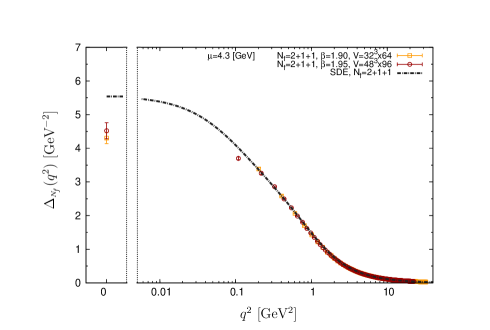
Figure 8: (color online) The unquenched gluon propagators obtained from our analysis, for $N_{\!f}=2$ (upper panel) and $N_{\!f}=2+1+1$ (lower panel), compared with the lattice data of Ayala et al. (2012) for the same cases.

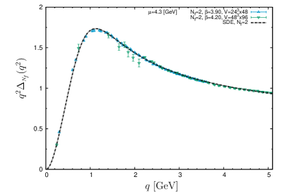
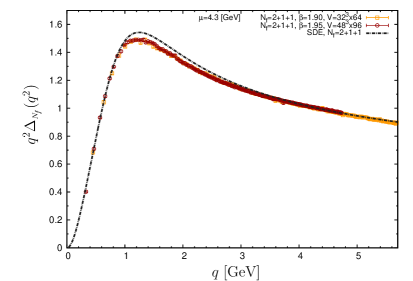
Figure 9: (color online) The gluon dressing functions, $q^{2}\Delta_{\scriptscriptstyle N_{\!f}}(q^{2})$, corresponding to the propagators of the previous figure.

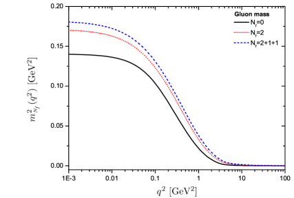
Figure 10: (color online) Solution of the mass equation yielding the dynamically generated gluon mass for $N_{\!f}=2$ (red dotted line) and $N_{\!f}=2+1+1$ (blue dashed line). In the deep infrared one has $m_{2}(0)=413$ MeV, and $m_{2+1+1}(0)=425$ MeV. For comparison we also show the quenched gluon mass (black continuous line) obtained from the quenched lattice propagator, in which case $m(0)=376$ MeV.

In Fig. 7 we show how the procedure described above converges rather rapidly to a stable solution for both $\Delta_{\scriptscriptstyle N_{\!f}}(q^{2})$ (top panel) as well as $\lambda^{2}(q^{2})$ (bottom panel). In particular, observe that at the first iterative step one has $\lambda^{2}(q^{2})=0$; even though this gives rise to a propagator with the same saturation point as in the quenched case (red circles curve on the top panel), the presence of the fermion loops alter in a rather marked way the overall shape of the function. As discussed in the previous section, this affects in turn the kernel of the mass equation, resulting in a $\lambda^{2}(q^{2})>0$ already at the second step, which then forces the unquenched propagator to have a lower saturation point with respect to the quenched case (green stars curves on both panels). Notice that, as anticipated, $\lambda^{2}(q^{2})$ increases at each successive iteration, resulting in an unquenched propagator that is suppressed in the infrared with respect to the quenched case.

In Fig. 8 we present the central result of this analysis. In particular, we plot the propagators obtained when convergence of the above mentioned iteration procedure has been reached, and compare them with the corresponding unquenched lattice data, recently reported in Ayala et al. (2012). We observe a rather good agreement between our theoretical predictions and the lattice computation for both values of $N_{\!f}$, for the available range of physical momenta. A notable exception to this fair coincidence between curves is the saturation point of the $N_{\!f}=2+1+1$ case; specifically, the value obtained from our SDE analysis is 20% higher than that found in lattice simulations. Similar conclusions can be drawn by observing the plot corresponding to the gluon dressing function $q^{2}\Delta_{\scriptscriptstyle N_{\!f}}(q^{2})$ shown in Fig. 9: while one has an excellent agreement in the case of two degenerate light quarks, when two heavier quarks are added the SDE solution tends to mildly overestimate the amplitude of the characteristic peak located in the intermediate momentum region.

The corresponding dynamical gluon masses, $m^{2}_{2}(q^{2})$ and $m^{2}_{2+1+1}(q^{2})$, are shown in Fig. 10; for comparison, we also plot the quenched solution, $m^{2}(q^{2})$, obtained from Eq. (6) when the quenched lattice propagators of Bogolubsky et al. (2009) are used as input. In particular, the corresponding saturation points give $m_{2}(0)=413$ MeV and $m_{2+1+1}(0)=425$ MeV (at $\mu=4.3$ GeV), which should be compared with the value $m(0)=376$ MeV obtained for the quenched case. The results captured in  Fig. 10 are particularly important, because they demonstrate clearly that the mass generation mechanism established for pure Yang-Mills continues to operate in QCD-like circumstances.

Let us finally comment on some possible factors that might account for the aforementioned discrepancies between our predictions and the lattice data for $N_{\!f}=2+1+1$.

At first sight, one might be tempted to attribute part of the observed discrepancy to the presence of volume effects. Specifically, the propagator plot of Fig. 8 seems to indicate that the deviation happens in the deep IR region $q^{2}\lesssim 0.2$ GeV², where the lattice data are expected to be affected by moderate volume artifacts (see in particular Fig. 2 of Ayala et al. (2012)). However, a closer look at the corresponding gluon dressing function ( plot of Fig. 9) advocates against this possibility; indeed, one observes the onset of a noticeable discrepancy as early as $q^{2}\sim 2.8$ GeV², namely at a point where volume effects are well under control. Therefore it is reasonable to assume that the observed deviation is not lattice related, but signals rather a mild violation of one of the assumptions underlying the derivation of the unquenching formula (15).

In particular, it is natural to expect that one of our basic operating assumption, namely that the quark-loop contributions constitute a “perturbation” of the quenched propagator, will become progressively less accurate as the number of active flavors increases. It is therefore possible that from $N_{\!f}>2$ onward we begin to perceive the onset of additional effects, not captured by (15). For instance, the identification of the “pure” gluonic diagrams of the gluon SDE with the gluon propagator $\Delta(q^{2})$ obtained in quenched lattice simulations, may no longer be entirely reliable, due to the presence of (increasingly appreciable) effects, coming from higher-order quark subdiagrams.

Clearly, an additional theoretical uncertainty originates from the approximate (perturbative) treatment of the quantity $Y(k^{2})$. In particular, the parameter $C$ may only model, to some extent, unknown contributions that display a logarithmic momentum dependence, as in Eq. (19), but cannot account for terms with a different functional form. Moreover, the use of an Ansätz for the vertex $\widehat{\Gamma}_{\mu}$ entering into the definition of ${\widehat{X}}(q^{2})$ may induce further error, due to the fact that its transverse (automatically conserved part) is in general undetermined.

IV Conclusions

In this work we addressed the basic theoretical question of whether the mass generation mechanism established in pure Yang-Mills studies persists in real-world QCD. Specifically, by employing a methodology relying mainly on the SDEs that describe the gluon two-point sector within the PT-BFM framework, we studied in quantitative detail how the inclusion of dynamical quarks affects the generation of the momentum-dependent gluon mass, in the Landau gauge. This important issue is especially relevant and timely, given the qualitative picture that appears to emerge from recent unquenched lattice simulations. Our results demonstrate clearly that the gluon propagator still saturates in the infrared (therefore, a gluon mass is indeed generated), and that the saturation point is progressively suppressed, as the number of quark flavors increases.

Several of the salient dynamical features pertinent to the transition from the quenched to the unquenched theory have been presented in the preliminary study of Aguilar et al. (2012a). The main novelty of the present analysis resides in the fact that, unlike Aguilar et al. (2012a), where the saturation point of the gluon propagator was estimated by means of an extrapolation procedure, here it is determined explicitly from the solution of the gluon mass equation. Therefore, the results obtained constitute a genuine prediction of the formalism employed, emerging entirely from the inherent dynamical equations.

As has been explained in Aguilar et al. (2012a) and in the present work, the “lowest order unquenching” consists in including explicitly the contribution of the quark loop $\widehat{X}(q^{2})$, keeping all other quantities unquenched. This is reflected clearly at the level of the master formula Eq. (15), where the quantity $1+G(q^{2})$ (or, equivalently, $F^{-1}(q^{2})$, by virtue of Eq. (18)) assumes its quenched form, obtained from Bogolubsky et al. (2009). Moreover, the computation of $\widehat{X}(q^{2})$ [see Fig. 2] uses as input the quark propagator obtained from the gap equation, which, in turn, depends on both the gluon propagator and the ghost dressing function; again, the quenched forms of Bogolubsky et al. (2009) were employed. Finally, the strength of the gauge coupling $g$ also depends on the number of flavors; in the present analysis we have used its value when $N_{\!f}=0$ (momentum-subtraction scheme Boucaud et al. (2009)). In order to improve this analysis, and eventually reach a better agreement with the lattice, one possible strategy would be to gradually introduce quark effects into some of the aforementioned (quenched) ingredients. For example, one could envisage the possibility of using unquenched instead of quenched data for the ghost dressing function $F(q^{2})$, obtained from the lattice analysis of Ayala et al. (2012). Given that this quantity enters both in the master formula and the gap equation, its overall effect may be appreciable. In addition, the increase in the value of the gauge coupling produced by the inclusion of quark flavors may modify our predictions in the right directions. We hope to be able to implement some of these improvements in the near future.

It is worth pointing out that the ingredients obtained from the present analysis may be used to determine the flavor-dependence of the QCD effective charge, ${\overline{\alpha}}_{s}(q^{2})$. Specifically, as has been shown in Aguilar et al. (2009a), this latter quantity may be defined in terms of the functions $J(q^{2})$ and $G(q^{2})$, through the renormalization-group invariant combination ${\overline{\alpha}}^{\,-1}_{s}(q^{2})=\alpha_{s}^{-1}(\mu^{2})[1+G(q^{2};\mu^{2})]^{2}{J_{m}}(q^{2};\mu^{2})$, where $\mu$ is the renormalization (subtraction) point chosen, within an appropriate renormalization scheme. The direct determination of $J(q^{2})$ from its own dynamical equation, shown schematically in Eq. (6), is thwarted from the fact that the main ingredients entering in it are the fully dressed three-gluon vertex $BQ^{2}$ (studied in Binosi and Papavassiliou (2011)) and the (largely unexplored) four-gluon vertex $BQ^{3}$, for arbitrary values of their momenta. Instead, one may employ Eq. (4) to compute $J(q^{2})$ indirectly, using a combined approach based on the knowledge of the full propagator from the lattice, and the corresponding gluon mass from solving Eq. (7). (For the possibility of the direct extraction of the quantity ${\widehat{J}}_{m}(q^{2};\mu^{2})=[1+G(q^{2};\mu^{2})]^{2}{J_{m}}(q^{2};\mu^{2})$ from specialized lattice simulations, see Binosi et al. (2013)). Work in this direction is already in progress.

Finally, it would clearly be important to study the infrared dynamics of the gluon propagator, quenched and unquenched, away from the Landau gauge. The SDEs formulated within the PT-BFM framework provide a natural starting point for such an investigation in the continuum. In fact, it would be particularly relevant to determine whether the detailed mass generation mechanism established in the Landau gauge persists for other values of the gauge-fixing parameter, such as, for example, the Feynman gauge, which is known to be of central importance for the PT. To be sure, further reliable input from the lattice would be invaluable for accomplishing such a demanding task, given that, even though the formal procedure for implementing covariant $R_{\xi}$ gauges on the lattice has been already reported Cucchieri et al. (2009), the available simulations are restricted to modest size volumes, and $\xi\ll 1$ only Cucchieri et al. (2010). We hope to report progress in some of these directions in the near future.