Asymptotic properties of the MLE for the autoregressive process coefficients under stationary Gaussian noise

Abstract

In this paper we are interested in the Maximum Likelihood Estimator (MLE) of the vector parameter of an autoregressive process of order $p$ with regular stationary Gaussian noise. We exhibit the large sample asymptotical properties of the MLE under very mild conditions. Simulations are done for fractional Gaussian noise (fGn), autoregressive noise (AR(1)) and moving average noise (MA(1)).

1 Statement of the problem

1.1 Introduction

The problem of parametric estimation in classical autoregressive (AR) models generated by white noises noises has been studied for decades. In particular, for such autoregressive models of order $1$ (AR(1)) consistency and many other asymptotic properties (distribution, bias, quadratic error) of the Maximum Likelihood Estimator (MLE) have been completely analyzed in all possible cases: stable, unstable and explosive (see, e.g., [2, 4, 20, 21, 25, 26]). Concerning autoregressive models of order $p$ (AR(p)) with white noises, the results about the asymptotic behavior of the MLE are less exhaustive but there are still many contributions in the literature (see, e.g.,[2, 5, 12, 14, 17, 19]).

In the past thirty years numerous papers have been devoted to the statistical analysis of AR processes which may represent long memory phenomenons as encountered in various fields as econometrics [9], hydrology [13] or biology [18]. Of course the relevant models exit from the white noise frame evoked above and they involve more or less specific structures of dependence in the perturbations (see, e.g., [1, 7, 8, 10, 22, 28] for contributions and other references).

General conditions under which the MLE is consistent and asymptotically normal for stationary sequences have been given in [24]. In order to apply this result, it would be necessary to study the second derivatives of the covariance matrix of the observation sample $(X_{1},\ldots,X_{N})$. To avoid this difficulty, some authors followed an other approach suggested by Whittle [7] (which is not MLE) for stationary sequences. But even in autoregressive models of order $1$ as soon as $|\vartheta|>1$, the process is not stationary anymore and it is not possible to apply theorems in [7] to deduce estimator properties.

In the present paper we deal with an AR(p) model generated by an arbitrary regular stationary Gaussian noise. We exhibit an explicit formula for the MLE of the parameter and we analyze its asymptotic properties.

1.2 Statement of the problem

We consider an AR(p) process $(X_{n},\,n\geq 1)$ defined by the recursion

$$X_{n}=\sum_{i=1}^{p}\vartheta_{i}X_{n-i}+\xi_{n},\quad n\geq 1,\quad X_{r}=0,\quad r=0,\,-1,\ldots,\,-(p-1),$$ (1)

where $\xi=(\xi_{n},\,n\in\mathbb{Z})$ is a centered regular stationary Gaussian sequence, i.e.

$$\int_{-\pi}^{\pi}\left|\ln f_{\xi}(\lambda)\right|d\lambda<\infty,$$ (2)

where $f_{\xi}(\lambda)$ is the spectral density of $\xi$. We suppose that the covariance $c=(c(m,n),\,m,n\geq 1)$, where

$$\mathbf{E}\xi_{m}\xi_{n}=c(m,\,n)=\rho(|n-m|),\quad\rho(0)=1,$$ (3)

is positive defined.

For a fixed value of the parameter $\vartheta=(\vartheta_{1},\,\dots,\,\vartheta_{p})\in\mathbb{R}^{p}$, let $\mathbf{P}_{\vartheta}^{N}$ denote the probability measure induced by $X^{(N)}$. Let $\mathcal{L}(\vartheta,\,X^{(N)})$ be the likelihood function defined by the Radon-Nikodym derivative of $\mathbf{P}_{\vartheta}^{N}$ with respect to the Lebesgue measure. Our goal is to study the large sample asymptotical properties of the Maximum Likelihood Estimator (MLE) $\widehat{\vartheta}_{N}$ of $\vartheta$ based on the observation sample $X^{(N)}=\left(X_{1},\ldots,X_{N}\right)$:

$$\hat{\vartheta}_{N}=\sup_{\vartheta\in\mathbb{R}^{p}}\mathcal{L}(\vartheta,\,X^{(N)}).$$ (4)

At first, preparing for the analysis of the consistency (or strong consistency) of $\hat{\vartheta}_{N}$ and its limit distribution we transform our observation model into an ”equivalent” model with independent Gaussian noises. This allows to write explicitly the MLE and actually, the difference between $\hat{\vartheta}_{N}$ and the real value $\vartheta$ appears as the product of a martingale by the inverse of its bracket process. Then we can use Laplace transforms computations to prove the asymptotical properties of the MLE.

The paper is organized as follows. Section  2 contains theoretical results and simulations. Sections  3 and 4 are devoted to preliminaries and auxiliary results. The proofs of the main results are presented in Section  5.

Acknowledgments

We would like to thank Alain Le Breton for very fruitful discussions and his interest for this work.

2 Results and illustrations

2.1 Results

We define the $p\times p$ companion matrix $A_{0}$ and the vector $b\in\mathbb{R}^{p}$ as follows:

$$A_{0}=\left(\begin{array}[]{ccccc}\vartheta_{1}&\vartheta_{2}&\cdots&\vartheta_{p-1}&\vartheta_{p}\\ 1&0&\cdots&0&0\\ 0&1&\cdots&0&0\\ \vdots&\vdots&\ddots&\vdots&\vdots\\ 0&0&\cdots&1&0\\ \end{array}\right),\quad b=\left(\begin{array}[]{c}1\\ \mathbf{0}_{(p-1)\times 1}\\ \end{array}\right).$$ (5)

Let $r(\vartheta)$ be the spectral radius of $A_{0}$. The following results hold:

Theorem 2.1.

Let $p\geq 1$ and the parameter set be:

$$\Theta=\left\{\vartheta\in\mathbb{R}^{p}\,|\,r(\vartheta)<1\right\}.$$ (6)

The MLE $\hat{\vartheta}_{N}$ is consistent, i.e., for any $\vartheta\in\Theta$ and $\nu>0$,

$$\lim_{N\rightarrow\infty}\mathbf{P}_{\vartheta}^{N}\left\{\left\|\hat{\vartheta}_{N}-\vartheta\right\|>\nu\right\}=0\,,$$ (7)

and asymptotically normal

$$\sqrt{N}\left(\hat{\vartheta}_{N}-\vartheta\right)\overset{\textit{law}}{\Rightarrow}\mathcal{N}(\mathbf{0},\,\mathcal{I}^{-1}(\vartheta)),$$ (8)

where $\mathcal{I}(\vartheta)$ is the unique solution of the Lyapounov equation:

$$\mathcal{I}(\vartheta)=A_{0}\mathcal{I}(\vartheta)A_{0}^{*}+bb^{*},$$ (9)

for $A_{0}$ and $b$ defined in (5).

Moreover we have the convergence of the moments: for any $\vartheta\in\Theta$ and $q>0$

$$\lim_{N\rightarrow\infty}\left|\mathbf{E}_{\vartheta}\left\|\sqrt{N}\left(\hat{\vartheta}_{N}-\vartheta\right)\right\|^{q}-\mathbf{E}\left\|\eta\right\|^{q}\right|=0,$$ (10)

where $\|\,\|$ denotes the Euclidian norm on $\mathbb{R}^{p}$ and $\eta$ is a zero mean Gaussian random vector with covariance matrix ${\cal I}(\vartheta)^{-1}.$

Remark 2.1.

It is worth to emphasize that the asymptotic covariance $\mathcal{I}^{-1}(\vartheta)$ is actually the same as in the standard case where $(\xi_{n})$ is a white noise. (cf. [?]).

In the case $p=1$ we can strengthen the assertions of Theorem 2.1. In particular, the strong consistency and uniform convergence on compacts of the moments hold.

Theorem 2.2.

Let $p=1$ and the parameter set be $\Theta=\mathbb{R}.$ The MLE $\hat{\vartheta}_{N}$ is strongly consistent, i.e. for any $\vartheta\in\Theta$

$$\lim_{N\rightarrow\infty}\hat{\vartheta}_{N}=\vartheta\quad\quad a.s..$$ (11)

Moreover, $\hat{\vartheta}_{N}$ is uniformly consistent and satisfies the uniform convergence of the moments on compacts $\mathbbm{K}\subset(-1,\,1)$, i.e. for any $\nu>0:$

$$\lim_{N\rightarrow\infty}\sup_{\vartheta\in\mathbb{K}}\mathbf{P}_{\vartheta}^{N}\left\{\left|\hat{\vartheta}_{N}-\vartheta\right|>\nu\right\}=0\,,$$ (12)

and for any $q>0:$,

$$\lim_{N\rightarrow\infty}\sup_{\vartheta\in\mathbb{K}}\left|\mathbf{E}_{\vartheta}\left|\sqrt{N}\left(\hat{\vartheta}_{N}-\vartheta\right)\right|^{q}-\mathbf{E}\left|\eta\right|^{q}\right|=0,$$ (13)

where $\eta\sim\mathcal{N}(0,\,1-\vartheta^{2}).$

Remark 2.2.

It is worth mentioning that condition (2) can be rewritten in terms of the covariance function $\rho$ : $\rho(n)\sim n^{-\alpha},\,\alpha>0$.

2.2 Simulations

In this section we present for $p=1$ three illustrations of the behavior of the MLE corresponding to noises which are MA(1), AR(1) and fGn.

Moving average noise MA(1)

Here we consider MA(1) noises where

$$\xi_{n+1}=\frac{1}{\sqrt{1+\alpha^{2}}}(\varepsilon_{n+1}+\alpha\varepsilon_{n}),\quad n\geq 1,$$

where $(\varepsilon_{n},n\geq 1)$ is a sequence of i.i.d. zero-mean standard Gaussian variables. Then the covariance function is given by

$$\rho(|n-m|)=\mathbbm{1}_{\{|n-m|=0\}}+\frac{\alpha}{1+\alpha^{2}}\mathbbm{1}_{\{|n-m|=1\}}.$$

Condition (2) is fulfilled for $|\alpha|<1$.

Autoregressive noise (AR(1))

Here we consider stationary autoregressive AR(1) noises where

$$\xi_{n+1}=\sqrt{1-\alpha^{2}}\varepsilon_{n+1}+\alpha\xi_{n},\quad n\geq 1,$$

where $(\varepsilon_{n},n\geq 1)$ is a sequence of i.i.d. zero-mean standard Gaussian variables. Then the covariance function is

$$\rho(|n-m|)=\alpha^{|n-m|}.$$

Condition (2) is fulfilled for $|\alpha|<1$.

Fractional Gaussian noise fGn

Here the covariance function of $(\xi_{n})$ is

$$\rho(|m-n|)=\frac{1}{2}\left(|m-n+1|^{2H}-2|m-n|^{2H}+|m-n-1|^{2H}\right),$$

for a known Hurst exponent $H\in(0,1).$ For simulation of the fGn we use Wood and Chan method (see [27]). The explicit formula for the spectral density of fGn sequence has been exhibited in [23]. Condition (2) is fulfilled for any $H\in(0,1).$

On Figure 1 we can see that in conformity with Theorem 2.2, in the three cases the MLE is asymptotically normal with the same limiting variance as in the classical i.i.d. case.

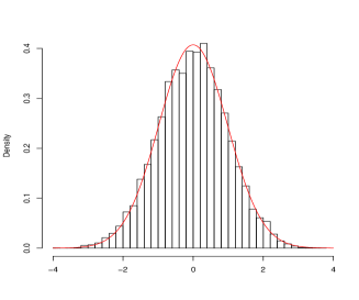
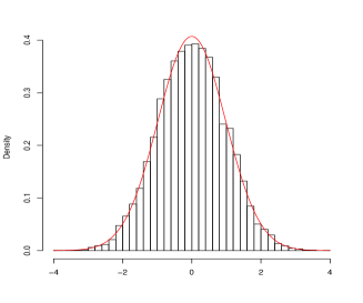
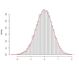
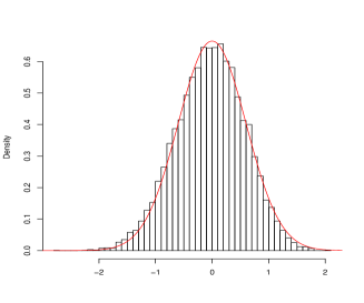
Figure 1: Asymptotical normality $N=2000$ for the MLE in different cases by Monte-Carlo simulation of $M=10000$ independent replications for AR(1) noises (top left) and MA noises (top right), both for $\alpha=0.4$ and $\vartheta=0.2$, and fGn noises for $H=0.2$ (bottom left) and for $H=0.8$ (bottom right) both for $\vartheta=0.8$.

3 Preliminaries

3.1 Stationary Gaussian sequences

We begin with some well known properties of a stationary scalar Gaussian sequence $\xi=(\xi_{n})_{n\geq 1}$. We denote by $(\sigma_{n}\varepsilon_{n})_{n\geq 1}$ the innovation type sequence of $\xi$ defined by

$$\sigma_{1}\varepsilon_{1}=\xi_{1},\quad\sigma_{n}\varepsilon_{n}=\xi_{n}-\mathbf{E}(\xi_{n}\,|\,\xi_{1},\dots,\xi_{n-1}),\quad n\geq 2,$$

where $\varepsilon_{n}\sim\mathcal{N}(0,1)$, $n\geq 1$ are independent. It follows from the Theorem of Normal Correlation ([16], Theorem 13.1) that there exists a deterministic kernel denoted by $k(n,m)$, $n\geq 1$, $m\leq n$, such that

$$\sigma_{n}\varepsilon_{n}=\sum_{m=1}^{n}k(n,m)\xi_{m},\quad k(n,n)=1.$$ (14)

In the sequel, for $n\geq 1$, we denote by $\beta_{n-1}$ the partial correlation coefficient

$$-k(n,1)=\beta_{n-1},\,n\geq 1.$$ (15)

The following relations between $k(\cdot,\,\cdot)$, the covariance function $\rho(\cdot)$ defined by (3), the sequence of partial correlation coefficients $\left(\beta_{n}\right)_{n\geq 1}$ and the variances of innovations $\left(\sigma_{n}^{2}\right)_{n\geq 1}$ hold (see Levinson-Durbin algorithm [6])

$$\sigma_{n}^{2}=\prod_{m=1}^{n-1}(1-\beta_{m}^{2}),\quad n\geq 2,\quad\sigma_{1}=1,$$ (16)

$$\sum_{m=1}^{n}k(n,\,m)\rho(m)=\beta_{n}\sigma_{n}^{2},$$ (17)

$$k(n+1,\,n+1-m)=k(n,\,n-m)-\beta_{n}k(n,\,m).$$ (18)

Since we assume the positive definiteness of the covariance $c(\cdot,\,\cdot)$, there also exists an inverse deterministic kernel $K=(K(n,\,m),\,n\geq 1,\,m\leq n)$ such that

$$\xi_{n}=\sum_{m=1}^{n}K(n,m)\sigma_{m}\varepsilon_{m}.$$ (19)

Remark 3.1.

Actually, kernels $k$ and $K$ are nothing but the ingredients of the Choleski decomposition of covariance and inverse of covariance matrices. Namely,

$$\Gamma_{n}^{-1}=k_{n}D_{n}^{-1}k_{n}^{*}\quad\mbox{and}\quad\Gamma_{n}=K_{n}^{*}D_{n}K_{n},$$

where $\Gamma_{n}=((\rho(|i-j|)))$ , $k_{n}$ and $K_{n}$ are $n\times n$ lower triangular matrices with ones as diagonal entries and $k(i,j)$ and $K(i,j)$ as subdiagonal entries respectively and $D_{n}$ is an $n\times n$ diagonal matrix with $\sigma_{i}^{2}$ as diagonal entries. Here $*$ denotes the transposition.

Remark 3.2.

It is worth mentioning that condition (2) implies that

$$\sum_{n\geq 1}\beta_{n}^{2}<\infty.$$ (20)

Indeed, for every regular stationary Gaussian sequence $\xi=(\xi_{n},\,n\in\mathbb{Z})$, there exists a sequence of i.i.d $\mathcal{N}(0,1)$ random variables $(\widetilde{\varepsilon}_{n},\,n\in\mathbb{Z})$ and a sequence of real numbers $a_{k},\,k\geq 0$ with $a_{0}\neq 0$ such that:

$$\xi_{n}=\sum_{k=0}^{\infty}a_{k}\widetilde{\varepsilon}_{n-k},$$

and for all $n\in\mathbb{Z}$ the $\sigma$-algebra generated by $(\xi_{k})_{-\infty<k\leq n}$ coincides with the $\sigma$-algebra generated by $(\widetilde{\varepsilon}_{k})_{-\infty<k\leq n}.$

Note that the variance $\sigma_{n}^{2}$ of the innovations is also the one step predicting error and the following equalities hold thanks to the stationarity of $\xi$:

$$\lim_{n\rightarrow\infty}\prod_{m=1}^{n-1}(1-\beta_{m}^{2})=\lim_{n\rightarrow\infty}\sigma_{n}^{2}$$

$$=\lim_{n\rightarrow\infty}\mathbf{E}\left(\xi_{n}-\mathbf{E}(\xi_{n}|\xi_{1},\cdots\xi_{n-1})\right)^{2}=\lim_{n\rightarrow\infty}\mathbf{E}\left(\xi_{0}-\mathbf{E}(\xi_{0}|\xi_{-1},\cdots\xi_{-n+1})\right)^{2}$$

$$=\mathbf{E}\left(\xi_{0}-\mathbf{E}(\xi_{0}|\xi_{s},s\leq-1)\right)^{2}=\mathbf{E}\left(\xi_{0}-\mathbf{E}(\xi_{0}|\varepsilon_{s},s\leq-1)\right)^{2}=a_{0}^{2}>0$$

which implies (20).

3.2 Model Transformation

As usual, for the first step we extend the dimension of the observations in order to work with a first order autoregression in $\mathbb{R}^{p}$. Namely, let $Y_{n},\,n\geq 1,$ be $Y_{n}=(X_{n},\,X_{n-1},\,\dots,\,X_{n-(p-1)})^{*}$ then $Y=(Y_{n},\,n\geq 1)$ satisfies the first order autoregressive equation:

$$Y_{n}=A_{0}Y_{n-1}+b\xi_{n},\quad n\geq 1,\quad Y_{0}=\mathbf{0}_{p\times 1},$$ (21)

where $A_{0}$ and $b$ are defined in (5). For the second step we take an appropriate linear transformation of $Y$ in order to have i.i.d. noises in the corresponding observations. For this goal let us introduce the process $Z=\left(Z_{n},n\geq 1\right)$ such that

$$Z_{n}=\sum_{m=1}^{n}k(n,\,m)Y_{m},\quad n\geq 1,$$ (22)

where $k=(k(n,\,m),\,n\geq 1,\,m\leq n)$ is the kernel appearing in (14). Since we have also

$$Y_{n}=\sum_{m=1}^{n}K(n,m)Z_{m},$$ (23)

where $K=(K(n,\,m),\,n\geq 1,\,m\leq n)$ is the inverse kernel of $k$ (see (19)), the filtration of $Z$ coincides with the filtration of $Y$ (and also the filtration of $X$). Actually, it was shown in [3] that $Z$ can be considered as the first component of a $2p$ dimensional $AR(1)$ process $\zeta=(\zeta_{n},\,n\geq 1)$ governed by i.i.d. noises. More precisely, the process $\zeta=(\zeta_{n},\,n\geq 1)$ defined by :

$$\zeta_{n}=\begin{pmatrix}Z_{n}\\ \displaystyle\sum_{r=1}^{n-1}\beta_{r}Z_{r}\end{pmatrix},$$

is a 2p-dimensional Markovian process which satisfies the following equation:

$$\zeta_{n}=\mathbf{A}_{n-1}\zeta_{n-1}+\ell\sigma_{n}\varepsilon_{n},\quad\,n\geq 1,\,\quad\zeta_{0}=\mathbf{0}_{2p\times 1},$$ (24)

where

$$\mathbf{A}_{n}=\left(\begin{array}[]{cc}A_{0}&\beta_{n}A_{0}\\ \beta_{n}\mathbf{Id}_{p\times p}&\mathbf{Id}_{p\times p}\\ \end{array}\right),\quad\ell=\left(\begin{array}[]{c}1\\ \mathbf{0}_{(2p-1)\times 1}\\ \end{array}\right),$$ (25)

and $(\varepsilon_{n},\,n\geq 1)$ are i.i.d. zero mean standard Gaussian variables. Now the initial estimation problem is replaced by the problem of estimation of the unknown parameter $\vartheta$ from the observations of $\zeta=(\zeta_{n},\,n\geq 1)$.

3.3 Maximum Likelihood Estimator

It follows directly from equation (24) that the log-likelihood function is nothing but:

$$\ln\mathcal{L}(\vartheta,\,X^{(N)})=-\frac{1}{2}\sum_{n=1}^{N}\left(\frac{\ell^{*}(\zeta_{n}-\mathbf{A}_{n-1}\zeta_{n-1})}{\sigma_{n}}\right)^{2}-\frac{N}{2}\ln 2\pi-\frac{1}{2}\sum_{n=1}^{N}\ln\sigma_{n}^{2}$$

and that the maximum likelihood estimator $\hat{\vartheta}_{N}$ is:

$$\hat{\vartheta}_{N}=\left(\sum_{n=1}^{N}\frac{a_{n-1}^{*}\zeta_{n-1}\zeta_{n-1}^{*}a_{n-1}}{\sigma_{n}^{2}}\right)^{-1}\cdot\left(\sum_{n=1}^{N}\frac{a_{n-1}^{*}\zeta_{n-1}\ell^{*}\zeta_{n}}{\sigma_{n}^{2}}\right).$$ (26)

Then we can write

$$\hat{\vartheta}_{N}-\vartheta=\left(\langle M\rangle_{N}\right)^{-1}\cdot M_{N},$$ (27)

where

$$M_{N}=\sum_{n=1}^{N}\frac{a_{n-1}^{*}\zeta_{n-1}}{\sigma_{n}}\varepsilon_{n}\,,\quad\quad\langle M\rangle_{N}=\sum_{n=1}^{N}\frac{a_{n-1}^{*}\zeta_{n-1}\zeta_{n-1}^{*}a_{n-1}}{\sigma_{n}^{2}},$$ (28)

with

$$a_{n}=\left(\begin{array}[]{c}\mathbf{Id}_{p\times p}\\ \beta_{n}\mathbf{Id}_{p\times p}\end{array}\right).$$ (29)

Note that $(M_{n},\,n\geq 1)$ is a martingale and $(\langle M\rangle_{n},\,n\geq 1)$ is its bracket process.

Remark 3.3.

It is worth mentioning that in the classical i.i.d. case, i.e., when $\beta_{n}=0,\,n\geq 1,$ $M_{N}$ and $\langle M\rangle_{N}$ in equations (27)-(28) reduce to:

$$M_{N}=\sum_{n=1}^{N}Y_{n-1}\varepsilon_{n}\,,\quad\quad\langle M\rangle_{N}=\sum_{n=1}^{N}Y_{n-1}Y_{n-1}^{*}.$$

Of course, under the condition $r(\vartheta)<1$ due to the law of the large numbers and the central limit theorem for martingales the following convergences hold:

$$\mathbf{P}_{\vartheta}-\lim_{N\rightarrow\infty}\frac{1}{N}\langle M\rangle_{N}=\mathcal{I}(\vartheta),\,\frac{1}{\sqrt{N}}M_{N}\overset{\textit{law}}{\Rightarrow}\mathcal{N}\left(\mathbf{0},\,\mathcal{I}(\vartheta)\right),$$ (30)

where $\mathcal{I}(\vartheta)$ is the unique solution of the Lyapounov equation (9). This implies immediately the consistency and the asymptotic normality of the MLE.

4 Auxiliary results

Actually, the proof of Theorems 2.1- 2.2 is crucially based on the asymptotic study for $N$ tending to infinity of the Laplace transform:

$$L_{N}^{\vartheta}(\mu)=\mathbf{E}_{\vartheta}\exp\left(-\frac{\mu}{2}\alpha^{*}\langle M\rangle_{{}_{N}}\alpha\right),$$ (31)

for arbitrary $\alpha\in\mathbb{R}^{p}$ and a positive real number $\mu$, where $\langle M\rangle_{N}$ is defined by (28). It can be rewritten as

$$L_{N}^{\vartheta}(\mu)=\mathbf{E}_{\vartheta}\exp\left(-\frac{\mu}{2}\sum_{n=1}^{N}\zeta_{n}^{*}{\cal M}_{n}\zeta_{n}\right),$$ (32)

where $\mathcal{M}_{n}=\displaystyle{\frac{1}{\sigma_{n+1}^{2}}}a_{n}\alpha\alpha^{*}a_{n}^{*}$, $a_{n}$ is defined by (29) and $\zeta$ satisfies the equation (24). In the sequel we will suppose that all the eigenvalues of $A_{0}$ are simple and different from $0$. Actually, it is not a real restriction, since the general case can be studied by using small perturbations arguments.

Lemma 4.1.

The Laplace transform $L_{N}^{\vartheta}(\mu)$ can be written explicitly in the following form:

$$L_{N}^{\vartheta}(\mu)=\left(\left(\prod_{n=1}^{N}\det\mathbf{A}_{n}\right)\det\Psi^{1}_{N}\right)^{-\frac{1}{2}},$$ (33)

where $\mathbf{A}_{n}$ is defined by equation (25) and

$$\sigma_{N+1}^{2}\Psi_{N}^{1}=\Psi_{0}\mathbf{J}\prod_{n=1}^{N}(\mathcal{A}_{\mu}\otimes A_{1}^{n}+\mathbf{Id}_{2p\times 2p}\otimes A_{2}^{n})\mathbf{J^{*}}\Psi_{0}^{*}.$$ (34)

Here $\otimes$ is the Kronecker product, $\Psi_{0}=(\mathbf{Id}_{2p\times 2p}\quad\mathbf{0}_{2p\times 2p})$,

$$\mathcal{A}_{\mu}=\left(\begin{array}[]{cc}A_{0}^{-1}&A_{0}^{-1}bb^{*}\\ \mu\alpha\alpha^{*}&A_{0}^{*}+\mu\alpha\alpha^{*}A_{0}^{-1}bb^{*}\\ \end{array}\right)$$ (35)

and $2\times 2$ matrices $A_{1}^{n},\,A_{2}^{n}$ are defined by

$$A_{1}^{n}=\left(\begin{array}[]{cc}1&0\\ -\beta_{n}&0\\ \end{array}\right),\quad\quad A_{2}^{n}=\left(\begin{array}[]{cc}0&-\beta_{n}\\ 0&1\\ \end{array}\right).$$ (36)

Proof.

The following equality can be proved by using the same arguments as those used in [11] (see equations (15) and (27)):

$$L_{N}^{\vartheta}(\mu)=\left(\left(\prod_{n=1}^{N}\det\mathbf{A}_{n}\right)\det\Psi^{1}_{N}\right)^{-\frac{1}{2}},$$

where $\Psi=((\Psi^{1}_{n},\Psi^{2}_{n}),\,n\geq 1)$ is the solution of the following equation:

$$\left\{\begin{array}[]{rrrrrrrl}\Psi^{1}_{n-1}&=&\Psi^{1}_{n}\mathbf{A}_{n}&-&\mu\Psi_{n-1}^{2}{\cal M}_{n-1},&\quad n\geq 1,\\ \Psi^{2}_{n}&=&\Psi^{1}_{n}\ell\ell^{*}\sigma_{n}^{2}&+&\Psi^{2}_{n-1}\mathbf{A}_{n}^{*},&\quad n\geq 1,\end{array}\right.$$

with the initial condition $\Psi_{0}=(\mathbf{Id}_{2p\times 2p}\quad\mathbf{0}_{2p\times 2p})$. This equation can be rewritten as

$$\left\{\begin{array}[]{rrrrrrrl}\Psi^{1}_{n}&=&\Psi^{1}_{n-1}\mathbf{A}_{n}^{-1}&+&\mu\Psi_{n-1}^{2}{\cal M}_{n-1}\mathbf{A}_{n}^{-1},&\quad n\geq 1,\\ \Psi^{2}_{n}&=&\Psi^{1}_{n-1}\mathbf{A}_{n}^{-1}\ell\ell^{*}\sigma_{n}^{2}&+&\Psi^{2}_{n-1}\left(\mu{\cal M}_{n-1}\mathbf{A}_{n}^{-1}\ell\ell^{*}\sigma_{n}^{2}+\mathbf{A}_{n}^{*}\right),&\quad n\geq 1.\end{array}\right.$$

Now let us denote by $\widetilde{\Psi}_{n}^{1}=\sigma_{n+1}^{2}\Psi_{n}^{1}$ and $\widetilde{\Psi}_{n}^{2}=\Psi_{n}^{2}\left(\begin{array}[]{cc}\mathbf{Id}_{p\times p}&\mathbf{0}_{p\times p}\\ \mathbf{0}_{p\times p}&-\mathbf{Id}_{p\times p}\\ \end{array}\right)$. Then $\widetilde{\Psi}_{n}=(\widetilde{\Psi}_{n}^{1}\quad\widetilde{\Psi}_{n}^{2})$ satisfies for $n\geq 1$ the following equation

$$\widetilde{\Psi}_{n}=\widetilde{\Psi}_{n-1}\left(\begin{array}[]{cccc}A_{0}^{-1}&-\beta_{n}\mathbf{Id}_{p\times p}&A_{0}^{-1}bb^{*}&\mathbf{0}_{p\times p}\\ -\beta_{n}A_{0}^{-1}&\mathbf{Id}_{p\times p}&-\beta_{n}A_{0}^{-1}bb^{*}&\mathbf{0}_{p\times p}\\ \mu\alpha\alpha^{*}A_{0}^{-1}&\mathbf{0}_{p\times p}&\mu\alpha\alpha^{*}A_{0}^{-1}bb^{*}+A_{0}^{*}&-\beta_{n}\mathbf{Id}_{p\times p}\\ -\beta_{n}(\mu\alpha\alpha^{*}A_{0}^{-1})&\mathbf{0}_{p\times p}&-\beta_{n}(\mu\alpha\alpha^{*}A_{0}^{-1}bb^{*}+A_{0}^{*})&\mathbf{Id}_{p\times p}\\ \end{array}\right).$$

Let $\pi$ be the following permutation of $\{1,\,\cdots,\,4p\}$ :

$$\pi(i)=\left\{\begin{array}[]{ll}k+1,&i=2k+1\\ p+r,&i=2r\par\\ 2p+k+1,&i=2p+2k+1\\ 3p+r,&i=2r+2p\end{array}\right.$$ (37)

where $k=0,\,\cdots,\,(p-1)$ and $r=1,\,\cdots,\,p$. Denote by $\mathbf{J}$ the correspond permutation matrix

$$\mathbf{J}_{ij}=\delta_{i\,\pi(j)},\quad i,j=1,\,\cdots,\,4p.$$

Then $\varphi_{n}=\widetilde{\Psi}_{n}\mathbf{J}$ satisfies the following equation:

$$\varphi_{n}=\varphi_{n-1}\left(\mathcal{A}_{\mu}\otimes A_{1}^{n}+\mathbf{Id}_{2p\times 2p}\otimes A_{2}^{n}\right),$$ (38)

which implies that

$$\varphi_{{}_{N}}=\Psi_{0}\mathbf{J}\prod_{n=1}^{N}(\mathcal{A}_{\mu}\otimes A_{1}^{n}+\mathbf{Id}_{2p\times 2p}\otimes A_{2}^{n}),$$

and consequently that $\sigma_{N+1}^{2}\Psi_{N}^{1}$ satisfies equality (34).

∎

Preparing for the asymptotic study we state the following result:

Lemma 4.2.

Let $(\beta_{n})_{n\geq 1}$ be a sequence of real numbers satisfying the condition (20). For a fixed real number $a$ let us define a sequence of $2\times 2$ matrices $(S_{N}(a))_{N\geq 1}$ such that:

$$S_{N}(a)=\prod_{n=1}^{N-1}\left(\begin{array}[]{cc}a&-\beta_{n}\\ -a\beta_{n}&1\\ \end{array}\right)=\prod_{n=1}^{N-1}(aA_{1}^{n}+A_{2}^{n}),$$ (39)

where $A_{1}^{n}$ and $A_{1}^{n}$ are defined by equation (36). Then

1. if $|a|<1,$ $\sup\limits_{N\geq 1}\|S_{N}(a)\|<\infty$,

2. if $|a|>1,$ $\sup\limits_{N\geq 1}\|(S_{N}(a))^{-1}\|<\infty$,

3. if $a$ is sufficiently small, $\inf\limits_{N\geq 1}\mbox{trace}((S_{N}^{-1}(\displaystyle{\frac{1}{a}}))S_{N}(a))>0$.

Proof.

The proof of assertions $1$ and $2$ follows directly from the estimates:

$$\|aA_{1}^{n}+A_{2}^{n}\|\leq 1+\beta_{n}^{2}\left(\frac{1+3a^{2}}{1-a^{2}}\right),\quad\quad\mbox{when}\quad|a|<1,$$

$$\|(aA_{1}^{n}+A_{2}^{n})^{-1}\|\leq 1+\beta_{n}^{2}\left(\frac{1+a^{2}}{a^{2}-1}\right),\quad\quad\mbox{when}\quad|a|>1.$$

The proof of assertion $3$ follows from the equality

$$G_{N}(a)=\frac{1}{1-\beta_{N}^{2}}\left(\begin{array}[]{cc}a&-\beta_{N}\\ -a\beta_{N}&1\\ \end{array}\right)G_{N-1}(a)\left(\begin{array}[]{cc}a&a\beta_{N}\\ \beta_{N}&1\\ \end{array}\right)$$

for $G_{n}(a)=S_{n}^{-1}(\displaystyle{\frac{1}{a}}))S_{n}(a)$. Hence $\mbox{trace}(G_{N}(0))=\displaystyle{\frac{1}{\sigma_{N}^{2}}}$ and condition (20) implies that $\displaystyle{\lim_{N\rightarrow\infty}\sigma_{N}^{2}=\prod_{n=1}^{\infty}\left(1+\beta_{n}^{2}\right)<\infty}$ which achieves the proof. ∎

Actually, in the asymptotic study we work with a small value of $\mu$. Note that for a small $\mu$, matrix $\mathcal{A}_{\mu}$ defined by (35) can be represented as: $\mathcal{A}_{\mu}=\mathcal{A}_{0}+\mu H$, where

$$\mathcal{A}_{0}=\left(\begin{array}[]{cc}A_{0}^{-1}&A_{0}^{-1}bb^{*}\\ \mathbf{0}_{p\times p}&A_{0}^{*}\\ \end{array}\right)\quad H=\left(\begin{array}[]{cc}\mathbf{0}_{p\times p}&\mathbf{0}_{p\times p}\\ \alpha\alpha^{*}&\alpha\alpha^{*}A_{0}^{-1}bb^{*}\\ \end{array}\right).$$ (40)

Representation (40) implies that if the spectral radius $r(\vartheta)<1$ then there are $p$ eigenvalues of $\mathcal{A}_{\mu}$ such that $|\lambda_{i}(\mu)|>1$ (in particular $\lambda_{i}(0),\,i=1,\,\cdots,\,p$ are the eigenvalues of $A_{0}^{-1}$) and $p$ eigenvalues of $\mathcal{A}_{\mu}$ such that $|\lambda_{j}(\mu)|<1,\,j=p+1,\,\cdots,\,2p.$

Lemma 4.3.

Suppose that $r(\vartheta)<1$. Let us take $\mu=\frac{1}{N}$ and denote by $\overline{L}_{N}^{\vartheta}(\mu)$:

$$\overline{L}_{N}^{\vartheta}(\mu)=\prod_{i=1}^{p}\left(\frac{\lambda_{i}(\mu)}{\lambda_{i}(0)}\right)^{-\frac{N}{2}}.$$ (41)

Then, under condition (2),

$$\lim_{N\rightarrow\infty}\frac{L_{N}^{\vartheta}(\mu)}{\overline{L}_{N}^{\vartheta}(\mu)}=1.$$ (42)

Proof.

Thanks to the definition (25) of $\mathbf{A}_{n}$ the equality

$$\prod_{n=1}^{N}\det\mathbf{A}_{n}=\prod_{n=1}^{N}\left[(1-\beta_{n}^{2})^{p}\frac{1}{\prod_{i=1}^{p}\lambda_{i}(0)}\right]=\frac{\left(\sigma_{N+1}^{2}\right)^{p}}{\prod_{i=1}^{p}\lambda_{i}(0)^{N}}$$

holds. Then due to equation (33) to prove (42) it is sufficient to check that

$$\lim_{N\rightarrow\infty}\frac{\det\sigma_{N+1}^{2}\Psi_{N}^{1}}{\left(\sigma_{N+1}^{2}\right)^{p}\prod_{i=1}^{p}[\lambda_{i}(\mu)]^{N}}=1.$$ (43)

Diagonalizing the matrix $\mathcal{A}_{\mu}$, i.e., representing $\mathcal{A}_{\mu}$ as $\mathcal{A}_{\mu}=G_{\mu}D(\lambda_{i}(\mu))G_{\mu}^{-1}$ with a diagonal matrix $D(\lambda_{i}(\mu))$, we have also

$$\mathcal{A}_{\mu}\otimes A_{1}^{n}+\mathbf{Id}_{2p\times 2p}\otimes A_{2}^{n}$$

$$=(G_{\mu}\otimes\mathbf{Id}_{2p\times 2p})(D(\lambda_{i}(\mu))\otimes A_{1}^{n}+\mathbf{Id}_{2p\times 2p}\otimes A_{2}^{n})(G_{\mu}^{-1}\otimes\mathbf{Id}_{2p\times 2p}).$$

This equation means that representation (34) can be rewritten as:

$$\sigma_{N+1}^{2}\Psi_{N}^{1}=\Psi_{0}\mathbf{J}(G_{\mu}\otimes\mathbf{Id}_{2p\times 2p})D(S_{N}(\lambda_{i}(\mu)))(G_{\mu}^{-1}\otimes\mathbf{Id}_{2p\times 2p})\mathbf{J^{*}}\Psi_{0}^{*},$$ (44)

where $D(S_{N}(\lambda_{i}(\mu)))$ is a block diagonal matrix with the block entries $S_{N}(\lambda_{i}(\mu)),\,i\leq 2p$ defined by equation (39). Since $G_{0}$ is a lower triangular matrix, it follows from (44) that

$$\sigma_{N+1}^{2}\Psi_{N}^{1}=P_{\mu}\mathcal{D}_{1}(S_{N}(\lambda_{i}(\mu)))Q_{\mu}+R_{\mu}\mathcal{D}_{2}(S_{N}(\lambda_{j}(\mu)))T_{\mu},$$

where

$$\lim_{\mu\rightarrow 0}P_{\mu}Q_{\mu}=\mathbf{Id}_{2p\times 2p},\quad\lim_{\mu\rightarrow 0}R_{\mu}=\mathbf{0}_{2p\times 2p},$$

and the block diagonal matrix $\mathcal{D}_{1}(S_{N}(\lambda_{i}))$ (respectively $\mathcal{D}_{2}(S_{N}(\lambda_{j}))$) is such that $|\lambda_{i}(\mu)|>1$ (respectively $|\lambda_{j}(\mu)|<1$ ).

Since $\det\mathcal{D}_{1}(S_{N}(\lambda_{i}(\mu)))=\left(\sigma_{N+1}^{2}\right)^{p}\prod_{i=1}^{p}[\lambda_{i}(\mu)]^{N}$ then, by Lemma 4.2 we get

$$\lim_{N\rightarrow\infty}\frac{\det\sigma_{N+1}^{2}\Psi_{N}^{1}}{\det\mathcal{D}_{1}(S_{N}(\lambda_{i}(\mu)))}=1,$$

which achieves the proof. ∎

The following statement plays a crucial role in the proofs.

Lemma 4.4.

Suppose that $r(\vartheta)<1$. Then under condition (2), for any $\alpha\in\mathbb{R}^{p}$,

$$\lim_{N\rightarrow\infty}L_{N}^{\vartheta}(\frac{1}{N})=\exp\left(-\frac{1}{2}\alpha^{*}\mathcal{I}(\vartheta)\alpha\right)$$ (45)

where $\mathcal{I}(\vartheta)$ is the unique solution of Lyapunov equation (9).

Proof.

It follows immediately from Lemma 4.3 that under condition (2) the limit of $L_{N}^{\vartheta}(\frac{1}{N})$ does not depend on the structure of noises $\xi$, i.e., does not depend on $\beta_{n}$. Thus, this limit is the same as for the classical i.i.d. situation, when $\beta_{n}=0,n\geq 1$.

∎

Remark 4.1.

It is worth mentioning that equation (41) says that

$$\sum_{i=1}^{p}\frac{d}{d\mu}\ln(\lambda_{i}(\mu))|_{\mu=0}=\alpha^{*}\mathcal{I}(\vartheta)\alpha,$$

where $\lambda_{i}(\mu)$ are the eigenvalues of $\mathcal{A}_{\mu}$ such that $|\lambda_{i}(\mu)|>1$ and $\mathcal{I}(\vartheta)$ is the solution of the Lyapunov equation (9). Of course, this equality can be proved independently.

5 Proofs

5.1 Proof of Theorem  2.1

The statement of Theorem follows from Lemma 4.4 since (45) implies immediately that

$$\mathbf{P}_{\vartheta}-\lim_{N\rightarrow\infty}\frac{1}{N}\langle M\rangle_{N}=\mathcal{I}(\vartheta),$$ (46)

and, hence also due to the central limit theorem for martingales,

$$\frac{1}{\sqrt{N}}M_{N}\overset{\textit{law}}{\Rightarrow}\mathcal{N}\left(\mathbf{0},\,\mathcal{I}(\vartheta)\right).$$

5.2 Proof of Theorem  2.2

Due to the strong law of large numbers for martingales, in order to proof the strong consistency we have only to check that

$$\lim_{N\rightarrow\infty}\langle M\rangle_{N}=+\infty\quad a.s.,$$

or, equivalently that for a one fixed constant $\mu>0$

$$\lim_{N\rightarrow\infty}\mathbf{E}_{\vartheta}\exp\left(-\frac{\mu}{2}\langle M\rangle_{N}\right)=0.$$ (47)

But in the case when $p=1$ the ingredients in the right hand side of formulas (33)- (34) with $\alpha=1$ can be given more explicitly:

$$\prod_{n=1}^{N}\det\mathbf{A}_{n}=\vartheta^{N}\sigma_{N+1}^{2},$$

and

$$\sigma_{N+1}^{2}\Psi_{N}^{1}=\frac{1-\lambda_{-}}{\lambda_{+}-\lambda_{-}}S_{N}(\frac{\lambda_{+}}{\vartheta})+\frac{\lambda_{+}-1}{\lambda_{+}-\lambda_{-}}S_{N}(\frac{\lambda_{-}}{\vartheta}),$$ (48)

where the matrix $S_{N}(a)$ is defined by equation (39),

$$\frac{\lambda_{\pm}}{\vartheta}=\frac{\vartheta^{2}+\mu+1\pm\sqrt{(\mu+(1-\vartheta)^{2})(\mu+(1+\vartheta)^{2})}}{2\vartheta}$$

are the two eigenvalues of the matrix $\displaystyle{\mathcal{A}_{\mu}=\left(\begin{array}[]{cc}\frac{1}{\vartheta}&\frac{1}{\vartheta}\\ \mu\frac{1}{\vartheta}&\mu\frac{1}{\vartheta}+\vartheta\\ \end{array}\right)}$ Note that $\displaystyle{\frac{\lambda_{+}}{\vartheta}\frac{\lambda_{-}}{\vartheta}=1,\,\left|\frac{\lambda_{+}}{\vartheta}\right|>1}$ and $\lambda_{+}>1$ for every $\mu>0$ and $\vartheta\in\mathbb{R}$. Equations (48) and (39) imply that for $\kappa=\frac{\lambda_{+}-1}{1-\lambda_{-}}$

$$\det\Psi_{N}^{1}=\left(\frac{1}{\sigma^{2}_{N+1}}\right)^{2}\left(\frac{1-\lambda_{-}}{\lambda_{+}-\lambda_{-}}\right)^{2}\det\left(S_{N}(\frac{\lambda_{+}}{\vartheta})\right)\det\left(\mathbf{Id}_{2\times 2}+\kappa(S_{N}(\frac{\lambda_{+}}{\vartheta}))^{-1}S_{N}(\frac{\lambda_{-}}{\vartheta})\right)$$

and that

$$\det\left(S_{N}(\frac{\lambda_{+}}{\vartheta})\right)=\vartheta^{-N}\lambda_{+}^{N}\sigma_{N+1}^{2}.$$

Thanks to Lemma 4.2

$$\det\left(\mathbf{Id}_{2\times 2}+\kappa(S_{N}(\frac{\lambda_{+}}{\vartheta}))^{-1}S_{N}(\frac{\lambda_{-}}{\vartheta})\right)$$

is uniformly bounded and separated from $0$ when $\mu$ is sufficiently large (and so $a=\frac{\lambda_{-}}{\vartheta}$ is sufficiently small). Since $\lambda_{+}>1$, we obtain that

$$\lim_{N\rightarrow\infty}L_{N}^{\vartheta}(\mu)=c\lim_{N\rightarrow\infty}\lambda_{+}^{-\frac{N}{2}}=0.$$

The uniform consistency and the uniform convergence of the moments on compacts $\mathbbm{K}\subset(-1,\,1)$ follow from the estimates (see [15], Eq.17.51):

$$\mathbf{E}_{\vartheta}\left(\frac{1}{N}\langle M\rangle_{N}\right)^{-q}\leq(1-\vartheta^{2})^{-q},$$

$$\mathbf{E}\left(\frac{1}{\sqrt{N}}M_{N}\right)^{q}\leq\left(\sqrt{1-\vartheta^{2}}\right)^{q}.$$

Remark 5.1.

It is worth mentioning that even in a stationary autoregressive models of order $1$ with strongly dependent noises the Least Square Estimator $\widetilde{\vartheta}_{N}=\frac{\sum_{n=1}^{N}X_{n-1}X_{n}}{\sum_{n=1}^{N}X^{2}_{n-1}}$ is not consistent.

References

- [1] J. Anděl. Long memory time series models. Kybernetika, 22(2):105–123, 1986.
- [2] T. W. Anderson. On asymptotic distribution of estimates of parameters of stochastic difference equations. Annals of Mathematical Statistics, 30:676–687, 1959.
- [3] A. Brouste and M. Kleptsyna. Kalman’s type filter under stationary noises. Systems and Control Letters, (1):517–532, 2012.
- [4] N. H. Chan and C. Z. Wei. Asymptotic inference for nearly non stationary AR(1) processes. Annals of Statistics, 15(3):1050–1063, 1987.
- [5] M. Duflo, R. Senoussi, and A. Touati. Propriétés asymptotiques presque sûres de l’estimateur des moindres carrés d’un modèle autorégressif vectoriel. Annales de l’Institut Henri Poincaré, 27(1):1–25, 1991.
- [6] J. Durbin. The fitting of time series models. Rev. Inst. Int. Stat., 28:233–243, 1960.
- [7] R. Fox and M. Taqqu. Large-sample properties of parameter estimates for strongly dependent stationary gaussian time series. The Annals of Statistics, 14(2):517–532, 1986.
- [8] C. W. Granger and R. Joyeux. An introduction to long-memory time series models and fractional differencing. Journal of Time Series Analysis, 1(1):15–29, 1980.
- [9] M. T. Greene and B. D. Fielitz. Long-term dependence in common stock returns. Journal of Financial Economics, 4(339–349), 1977.
- [10] J. R. M. Hosking. Fractional differencing. Biometrika, 68(1):165–176, 1981.
- [11] M. Kleptsyna, A. Le Breton, and M. Viot. New formulas concerning laplace transforms of quadratic forms for general gaussian sequences. Journal of Applied Mathematics and Stochastic Analysis, (1), 2002.
- [12] T. L. Lai and C. Z. Wei. Asymptotic properties of general autoregressive models and strong consistency of Least Square Estimate and their parameters. Journal of Multivariate Analysis, 13:1–23, 1983.
- [13] A. J. Lawrance and N. T. Kottegoda. Stochastic modeling of river flow time series. Journal of the Royal Statistical Society, 140(1–27), 1977.
- [14] A. Le Breton and D. T. Pham. On the bias of the least squares estimator for the first order autoregressive process. Ann. Inst. Statist. Math, 41(3):555–563, 1989.
- [15] R. Liptser and A. Shiryaev. Theory of Martingales. Kluwer Academic, 1989.
- [16] R. Liptser and A. Shiryaev. Statistics of Random Processes. Springer, 2001.
- [17] H. Mann and A. Wald. On the statistical treatment of linear stochastic difference equations. Econometrica, 11(3&4):173–220, 1943.
- [18] V. Maxim, L. Sendur, J. Fadili, J. Suckling, R. Gould, R. Howard, and E. Bullmore. Fractional gaussian noise, function MRI and Alzheimer’s disease. NeuroImage, 25(141-158), 2005.
- [19] M. M. Rao. Consistency and limit distributions of estimators of parameters in explosive stochastic difference equations. Annals of Mathematical Statistics, 32(1):195–218, 1961.
- [20] M. M. Rao. Asymptotic distribution of an estimator of the boundary parameter of an unstable process. Annals of Statistics, 6(1):185–190, 1978.
- [21] H. Rubin. Consistency of maximum-likelihood estimates in the explosive case. In Statistical Inference in Dynamic Economic Models, pages 356–364. John Wiley and Sons, New-York, 1950.
- [22] S. Sethuraman and I. V. Basawa. The asymptotic distribution of the maximum likelihood estimator for a vector time series model with long memory dependence. Statistics and Probability Letters, 31:285–293, 1997.
- [23] Y. G. Sinai. Self-similar probability distribution. Theory of probability and Its application, 21(1), 1976.
- [24] T. J. Sweeting. Uniform asymptotic normality of the maximum likelihood estimator. The Annalas of Statistics, 8:1375–1381, 1980.
- [25] J. White. The limiting distribution of the serial correlation coefficient in the explosive case. Annals of Mathematical Statistics, 29:1188–1197, 1958.
- [26] J. White. The limiting distribution of the serial correlation coefficient in the explosive case ii. Annals of Mathematical Statistics, 30:831–834, 1959.
- [27] A. Wood and G. Chan. Simulation of stationary gaussian processes. Journal of computational and graphical statistics, 3(4):409–432, 1994.
- [28] Y. Yajima. On estimation of long-memory time series models. Australian Journal of Statistics, 27(3):302–320–807, 1985.