Deformation and cluster structures in ¹²C studied with configuration mixing using Skyrme interactions

Abstract

We report an investigation of the structure of ¹²C nucleus employing a newly developed configuration-mixing method. In the three-dimensional coordinate-space representation, we generate a number of Slater determinants with various correlated structures using the imaginary-time algorithm. We then diagonalize a many-body Hamiltonian with the Skyrme interaction in the space spanned by the Slater determinants with parity and angular momentum projections. Our calculation reasonably describes the ground and excited states of ¹²C nucleus, both for shell-model-like and cluster-like states. The excitation energies and transition strengths of the ground-state rotational band are well reproduced. Negative parity excited states, $1_{1}^{-}$, $2_{1}^{-}$, and $3_{1}^{-}$, are also reasonably described. The second and third $0^{+}$ states, $0_{2}^{+}$ and $0_{3}^{+}$, appear at around 8.8 MeV and 15 MeV, respectively. The $0_{2}^{+}$ state shows a structure consistent with former results of the $\alpha$-cluster models, however, the calculated radius of the $0_{2}^{+}$ state is smaller than those calculations. The three-$\alpha$ linear-chain configuration dominates in the $0_{3}^{+}$ state.

I INTRODUCTION

Light nuclei show a variety of structures in the ground and excited states characterized by different correlations. The nuclear shell model usually provides a reasonable description for the ground and low-lying states. However, it is difficult for the shell model to describe well-developed cluster states which appear in excited states of light nuclei. The appearance of the cluster structures is intimately related to the small separation energy of clusters. This is called the threshold rule and has been described by the so-called Ikeda diagram Ikeda et al. (1968a).

For theoretical descriptions of cluster states, microscopic and semi-microscopic cluster models have been extensively developed in the past Ikeda and Tamagaki (1977); Ikeda et al. (1968b, 1980); Fujiwara et al. (1980). The resonating group method (RGM) Wheeler (1937a, b) assumes a product form for the wave function composed of the internal wave functions of clusters and the inter-cluster wave function, taking fully account of the antisymmetrization. The generator coordinate method (GCM) was also successfully applied to various cluster motions assuming harmonic oscillator shell-model wave functions for clusters. as well Brink and Weiguny (1968). In these microscopic models, the existence of clusters is assumed from the beginning. To understand mechanisms of emergence and disappearance of cluster structures, one should start with a model which does not assume any existence of clusters. Studies with the antisymmetrized molecular dynamics (AMD) method Kanada-En’yo and Horiuchi (1995); Kanada-En’yo et al. (1995); Kanada-En’yo (2007) have contributed to substantial advances in this direction. In most calculations with microscopic cluster models and AMD, effective nucleon-nucleon forces are used. In the Fermionic Molecular Dynamics (FMD) method which is closely related to the AMD, a more realistic force produced by the unitary correlation operator method has been employed Neff and Feldmeier (2004).

In last two decades, there have been significant advances in theoretical descriptions of light nuclei starting with realistic nucleon-nucleon force, so-called the ab-initio approach. The Green Function Monte Carlo (GFMC) approach has been successful to describe the ground and the low-lying excited states of light nuclei Carlson (1987). The GFMC calculation describes the two $\alpha$ cluster structure of ⁸Be in the ground state Wiringa et al. (2000). The no-core shell model (NCSM) has also been successful for the description of ground and low-lying excited states Navrátil et al. (2000, 2009). However, descriptions of cluster states in the NCSM have not yet been satisfactory. Recently there are a number of attempts for the ab-initio description of cluster structures in excited states. For example, a lattice calculation for the Hoyle state has been reported Epelbaum et al. (2011). The no-core shell model combined with Monte-Carlo basis generation method has also been applied Abe et al. (2012).

There are two important ingredients in the ab-initio descriptions of nuclear structures. One is to start with a Hamiltonian with a realistic nucleon-nucleon force that has a short-range repulsive core. The other is to obtain fully convergent solutions for the many-body Hamiltonian. Since cluster structures are characterized by long-range spatial correlations, simultaneous descriptions of both long- and short-range correlations are required in the ab-initio calculations of cluster states. This makes the problem computationally very challenging.

In this paper, we focus on the latter aspect of the above-mentioned problem, namely, on obtaining fully convergent solutions for a given many-body Hamiltonian, taking into account a variety of long-range correlations. We start not with a realistic nucleon-nucleon force but with an empirical effective interaction, the Skyrme force. We use a newly developed method which was reported previously Shinohara et al. (2006). We apply the method to ¹²C nucleus, then, examine descriptions of cluster structures. Since the Skyrme interaction is determined so as to reproduce nuclear properties of wide mass region, our calculation contains no empirical parameters specific to ¹²C.

Among light nuclei, the ¹²C nucleus is one of the most interesting systems for the reasons described below. In the $jj$ coupling shell-model picture, the ground state wave function should be dominated by the $p_{3/2}$ closed shell configuration. Indeed, the self-consistent Hartree-Fock solutions with most Skyrme interactions show a spherical shape with the $p_{3/2}$ closed shell configuration. However, the ¹²C nucleus is known to show a rotational band structure built on the ground state, indicating a deformed intrinsic shape in the ground state. In excited states, a variety of cluster structures are known to appear. The $0_{2}^{+}$ state just above the three-$\alpha$ decay threshold is an important resonant state for the triple-$\alpha$ fusion reaction, and is known as the Hoyle state Hoyle (1954). It has been found recently that this state is well described by a Bose condensed wave function of three-$\alpha$ particles which is called the THSR wave function Tohsaki et al. (2001); Funaki et al. (2003). The appearance of three-$\alpha$ linear-chain structure in excited states was suggested by Morinaga in 1966 Morinaga (1966). Recent microscopic cluster models predict that the $0_{3}^{+}$ state is a candidate for the linear-chain like structure Kanada-En’yo (2007); Neff and Feldmeier (2004).

This paper is organized as follows. In section II, we explain our method. In section III, we first show that we obtain convergent results for some low-lying states for the Skyrme Hamiltonian. We then describe in detail the calculated results for ¹²C. In section IV, we compare our results with conventional microscopic cluster model calculations by introducing cluster wave functions in our calculation. In section V, a summary is presented.

II Formulation

In this section, we present our formalism which was proposed in Ref. Shinohara et al. (2006). It is composed of three steps: We first generate a number of Slater determinants (SDs) in a stochastic way. These SDs are expected to span a sufficiently large model space to describe excited states with various cluster structures as well as low-lying states with shell-model-like structures. We then perform parity and angular momentum projections for the SDs. Finally we superpose them to diagonalize the Skyrme Hamiltonian. Below we describe these three steps of our formalism in order.

Before presenting our formalism, we briefly describe numerical aspects in the present method. For the energy functional, we employ the SLy4 parameter set of the Skyrme interaction unless otherwise specified. To describe single-particle orbitals of the SDs, we employ a representation of the three-dimensional (3D) Cartesian grid. This representation allows us a flexible description of single-particle orbitals in arbitrary nuclear shapes. The grid spacing is taken to be $\Delta x=\Delta y=\Delta z=0.8$ fm, and all the grid points inside a sphere of radius, $R_{\rm max}=8.0$ fm, are adopted.

II.1 Generation of Slater determinants

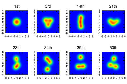
Figure 1: Contour plots of nuclear densities of the stored SDs for ¹²C. A sequential number of the SD is indicated in the top of the panel. Units of vertical and horizontal axes are fm.

The first step is to generate and select a sufficient number of SDs, $\{\Phi_{i}\}$ ($i=1,\cdots,M$), which span a large model space to describe various kinds of long-range correlations. To this end, we make use of the imaginary-time method with the Skyrme interaction. The imaginary-time method is usually used to obtain a ground-state solution in the mean-field calculation. Here, we use it for generation of many kinds of collective surfaces.

We start with initial SDs whose single-particle orbitals are described by the Gaussian wave packets,

$$\phi_{i}(\vec{r},\sigma)=e^{-|\vec{r}-\vec{R_{i}}(\sigma)|^{2}/a^{2}}.$$ (1)

The centers of the Gaussian wave packets, $\vec{R}_{i}(\sigma)$, are set by random numbers generated under the condition,

$$|\vec{R}_{i}(\sigma)|<R_{\rm max}-1\hskip 5.69054pt{\rm fm}.$$ (2)

The width parameter $a$ is taken to be 2 fm.

Then, we start the imaginary-time iterations with these initial SDs. During the imaginary-time iterations, we set constraints to place the center of mass at the origin and to make the principal axes of nuclei parallel to the Cartesian axes. After the sufficient number of iterations, it reaches the self-consistent ground-state solution, namely Hartree-Fock (HF) state. However, before reaching the HF solution, there appear a number of configurations which show various cluster structures and other configurations important for low-energy nuclear dynamics. Thus, we pick up and store these SDs which will be used for the configuration mixing calculation. We repeatedly perform the imaginary-time iterations starting with different initial SDs to obtain a sufficient number of SDs (typically 50) of many kinds of correlations.

In order to span a wide model space by the limited number of SDs, the actual selection of the SDs is achieved as follows: The first SD adopted in the basis set $\{\Phi_{i}\}$ is the HF state, $\Phi_{1}=\Phi_{\rm HF}$. The second and following SDs are generated as follows: During the imaginary-time iteration, the energy expectation value decreases monotonically. We examine the energy expectation value in a regular interval, typically every 100 iterations. We do not adopt the SD until the energy expectation value is less than 30 MeV above the HF ground-state energy. After the energy expectation value becomes less than this threshold, we examine the overlap between a current SD and previously selected ones. We denote the SDs which have been already selected as $\Phi_{i}(i=1,\cdots,N)$, and denote the current SD as $\Phi_{c}$. We calculate the quantities

$$\frac{\big{|}\big{<}\Phi_{i}|\hat{P}^{\pi}\hat{R}_{n}|\Phi_{c}\big{>}\big{|}}{\sqrt{\big{|}\big{<}\Phi_{i}|\hat{P}^{\pi}|\Phi_{i}\big{>}\big{|}}\sqrt{\big{|}\big{<}\Phi_{c}|\hat{P}^{\pi}|\Phi_{c}\big{>}\big{|}}}\hskip 5.69054pt(i=1,\cdots,N),$$ (3)

where $\hat{P}^{\pi}$ is the parity projection operator and $\hat{R}_{n}(n=1,\cdots,24)$ are operators of rotations and inversions which may be easily achieved by the changes of the coordinate axes. If the maximum value of the above overlap values between $\Phi_{c}$ and $\Phi_{i}(i=1,\cdots,N)$ is less than 0.7, we adopt the SD $\Phi_{c}$ as a new member, $\Phi_{N+1}=\Phi_{c}$. When the imaginary-time iteration reaches the self-consistent solution, we generate a new initial SD of the form of Eq. (1) and again start the imaginary-time iterations. We then repeat the procedure to select a new SD. We repeat the procedure until a sufficient number of SDs is obtained. Typically a few SDs are adopted during one imaginary-time iterations. As the number of stored SDs increases, it is more and more difficult to find the new SD which satisfies the overlap condition. In this way, we store SDs which include important correlation effects and which are linearly independent to each other as much as possible.

We show density distributions of several SDs generated in this procedure in Fig. 1. The numbers assigned to the figures, 1, 3, 14, 21, 23, 34, 39, and 50, simply indicates the adopted ordering. The first one which shows a spherical shape is the HF solution for the ground state. Other SDs in Fig. 1 show a variety of cluster structures. For example, $\Phi_{3}$ shows an equilateral triangular three-$\alpha$ structure, $\Phi_{14}$ shows a three-$\alpha$ linear-chain, and $\Phi_{23}$ shows a ⁸Be+$\alpha$ like structure. We thus observe that the present procedure efficiently produces SDs with various cluster structures in an automatic manner.

II.2 Projections of parity and angular momentum

The SDs prepared by the method in Sec. II.1 are, in general, not eigenstates of parity and angular momentum. To calculate matrix elements between eigenstates of parity and angular momentum, we apply the projection method. The projection operators are given as usual by

$$\hat{P}^{\pi} = \frac{1}{2}(1+(-1)^{\pi}\hat{P}_{r}),$$ (4)

$$\hat{P}^{J}_{MK} = \frac{2J+1}{8\pi^{2}}\int d\Omega D^{J*}_{MK}(\alpha,\beta,\gamma)\hat{R}(\alpha,\beta,\gamma),$$ (5)

where $\hat{P}_{r}$ is the space inversion operator, $\hat{R}(\alpha,\beta,\gamma)$ is the rotation operator for the Euler angles, $\alpha$, $\beta$, and $\gamma$, and $D^{J}_{MK}$ is the Wigner’s $D$-function defined by

$$\hat{R}(\alpha,\beta,\gamma) = e^{-i\alpha\hat{J}_{z}}e^{-i\beta\hat{J}_{y}}e^{-i\gamma J_{z}},$$ (6)

$$D^{J}_{MK}(\alpha,\beta,\gamma) = e^{-i\alpha M}d^{J}_{MK}(\beta)e^{-i\gamma K},$$ (7)

where $J$, $M$, and $K$ are the total angular momentum, its projection onto the laboratory $z$-axis, and its projection onto the body-fixed $z$-axis, respectively.

We define the norm and Hamiltonian matrix elements between the projected SDs $\big{|}\Phi_{i}\big{>}$ and $\big{|}\Phi_{j}\big{>}$ as

$$n^{J\pi}_{iK,jK^{\prime}}\equiv \frac{2J+1}{8\pi^{2}}$$

$$\times\int d\Omega D^{J*}_{KK^{\prime}}(\Omega)\big{<}\Phi_{i}\big{|}e^{-i\alpha\hat{J}_{z}}\hat{P}^{\pi}e^{-i\beta\hat{J}_{y}}e^{-i\gamma\hat{J}_{z}}\big{|}\Phi_{j}\big{>},$$ (8)

$$h^{J\pi}_{iK,jK^{\prime}}\equiv \frac{2J+1}{8\pi^{2}}$$

$$\times\int d\Omega D^{J*}_{KK^{\prime}}(\Omega)\big{<}\Phi_{i}\big{|}e^{-i\alpha\hat{J}_{z}}\hat{H}\hat{P}^{\pi}e^{-i\beta\hat{J}_{y}}e^{-i\gamma\hat{J}_{z}}\big{|}\Phi_{j}\big{>}.$$ (9)

Here, we use the formula,

$$\hat{P}^{J\dagger}_{MK}\hat{P}^{J}_{MK^{\prime}}=\hat{P}^{J}_{KK^{\prime}}.$$ (10)

In Eqs. (8) and (9), we need the rotation of wave functions. It is achieved by successive operations of small-angle rotations. For example, the rotation of a wave function $\phi$ over an angle $\gamma$ around the $z$-axis is achieved by successive rotations of a small angle, $\Delta\gamma=\gamma/N_{\gamma}$, $N_{\gamma}$ times,

$$e^{-i\gamma\hat{j}_{z}}\big{|}\phi\big{>}=\big{(}e^{-i\Delta\gamma\hat{j}_{z}}\big{)}^{N_{\gamma}}\big{|}\phi\big{>},$$ (11)

To achieve the small angle rotation, we employ the Taylor expansion method.

$$e^{-i\Delta\gamma\hat{j}_{z}}\big{|}\phi\big{>}\approx\sum^{N_{\rm max}}_{k=1}\frac{(-i\Delta\gamma\hat{j}_{z})^{k}}{k!}\big{|}\phi\big{>}.$$ (12)

Typically, we take $N_{\rm max}=4$ and $\Delta\gamma=\frac{\pi}{90}$.

The integrals over Euler angles in Eqs. (8) and (9) are evaluated as follows: Those over $\alpha$ and $\gamma$ are achieved by the trapezoidal rule, taking 18 uniform grid points for $[0,2\pi]$. The integral over $\beta$ is achieved with the Gauss-Legendre quadrature, taking 30 grid points for $[0,\pi]$.

II.3 Configuration mixing

The final procedure is diagonalization of the many-body Hamiltonian in the space spanned by the selected SDs. In Sec. II.1, the SDs have been screened by their linear independence. However, calculating eigenvalues of the norm matrix for the SDs after the parity and angular momentum projections, we find a number of eigenvalues very close to zero or even slightly negative. The norm matrix is positive definite by definition. However, since we make numerical approximations in evaluating the norm matrix, it could contain negative eigenvalues. The approximations include use of the formula for the product of the projection operators, Eq. (10), which is no longer exact if the integral over Euler angles is evaluated by the numerical quadrature. We also employ the 3D Cartesian grid representation for the orbitals in which the rotational symmetry holds only approximately.

Inclusion of those configurations of very small norm eigenvalues would lead to numerical difficulties. Therefore, we reduce the number of configurations according to the following procedures. First, we perform diagonalization in the $(2J+1)$-multiplet with different $K$ quantum numbers.

$$\sum_{K^{\prime}}n^{J\pi}_{iK,iK^{\prime}}v^{J\pi,i\nu}_{K^{\prime}}=e^{J\pi}_{i\nu}v^{J\pi,i\nu}_{K},\hskip 8.53581pt(\nu=1,\cdots,2J+1)$$ (13)

where $e^{J\pi}_{i\nu}$ and $v^{J\pi,i\nu}_{K}$ are eigenvalues and eigenvectors of the norm matrix, $n^{J\pi}_{iK,iK^{\prime}}$. We then construct a space spanned by the eigenvectors with the eigenvalue $e^{J\pi}_{i\nu}>10^{-2}$, and define the normalized basis functions

$$\big{|}\Phi^{J\pi}_{i\nu}\big{>}\equiv\frac{1}{\sqrt{e^{J\pi}_{i\nu}}}\sum_{K}v^{J\pi,i\nu}_{K}\hat{P}^{J}_{MK}\hat{P}^{\pi}\big{|}\Phi_{i}\big{>}.$$ (14)

After achieving the above procedure for all SDs, we define the following norm matrix between basis functions belonging to the different SDs,

$$\tilde{n}^{J\pi}_{i\nu,j\nu^{\prime}}\equiv\big{<}\Phi^{J\pi}_{i\nu}\big{|}\Phi^{J\pi}_{j\nu^{\prime}}\big{>}$$ (15)

Using this matrix, we examine the linear independence of the basis functions and reduce the number of basis as follows.

1. Calculate eigenvalues of $2\times 2$ matrices composed of every possible pair of basis functions, $(i_{1}\nu_{1})$ and $(i_{2}\nu_{2})$. If the smaller eigenvalue is less than $10^{-3}$, we remove the basis function with a smaller $e^{J\pi}_{i\nu}$.

2. Calculate the eigenvalues of $3\times 3$ matrices composed of three basis functions $(i_{1}\nu_{1})$, $(i_{2}\nu_{2})$ and $(i_{3}\nu_{3})$. If the smallest eigenvalue is less than $10^{-3}$, we remove one of the three basis functions in the following procedure. We calculate eigenvalues of three $2\times 2$ submatrices composed of all possible pairs of these three states, to find the pair whose smaller eigenvalue is the largest among the three. Then we remove one of the basis functions of $(i_{1}\nu_{1})$, $(i_{2}\nu_{2})$ and $(i_{3}\nu_{3})$ which does not belong to that pair. We repeat the procedure for all possible combinations of three basis functions.

3. Finally we calculate eigenvalues of the norm matrix $\tilde{n}^{J\pi}_{i\nu,j\nu^{\prime}}$ with basis functions which survived in the previous two screening steps. If we find the eigenvalue smaller than $10^{-3}$, we remove one basis function in the following way. Denoting the number of basis functions as $N$, we construct the $(N-1)\times(N-1)$ submatrices removing one basis function $\Phi_{i\nu}^{J\pi}$ from the $N$ basis. Apparently, $N$ different choices of $(i\nu)$ are possible. We then calculate the smallest eigenvalue of the $(N-1)\times(N-1)$ submatrix, $\lambda_{\rm min}^{(i\nu)}$. Among $\lambda_{\rm min}^{(i\nu)}$ with different $(i\nu)$, we find the largest one, $\lambda_{\rm min}^{(i^{\prime}\nu^{\prime})}$, and remove the basis function $\Phi_{i^{\prime}\nu^{\prime}}^{J\pi}$. In this way, the number of basis $\{\Phi_{i\nu}^{J\pi}\}$ is reduce by one, from $N$ to $N-1$. We repeat this process until the smallest eigenvalue of the norm matrix becomes larger than $10^{-3}$.

After removing the overcomplete basis functions in this procedure, we achieve the configuration mixing calculation. Denoting the $n$th energy eigenstate as

$$\big{|}\Psi^{J\pi}_{n}\big{>} = \sum_{i\nu}f_{i\nu}^{J\pi,n}\big{|}\Phi^{J\pi}_{i\nu}\big{>},$$ (16)

the generalized eigenvalue equation for the energy eigenvalues $E_{n}^{J\pi}$ and the coefficients $f_{i\nu}^{J\pi,n}$ is given by

$$\sum_{j\mu}\big{\{}\tilde{h}_{i\nu j\mu}^{J\pi}-E_{n}^{J\pi}\tilde{n}_{i\nu j\mu}^{J\pi}\big{\}}f_{j\mu}^{J\pi,n} = 0,$$ (17)

where $\tilde{h}^{J\pi}_{i\nu,j\nu^{\prime}}$ is defined by

$$\tilde{h}^{J\pi}_{i\nu,j\nu^{\prime}}\equiv\big{<}\Phi^{J\pi}_{i\nu}\big{|}\hat{H}\big{|}\Phi^{J\pi}_{j\nu^{\prime}}\big{>}.$$ (18)

III RESULTS

III.1 Convergence of results: Statistical treatment

In principle, the configuration mixing calculation with a sufficient number of SDs should provide unique and convergent energy levels. However, as we described in Sec. II, superposing a large number of non-orthogonal SDs causes numerical difficulties. In the present calculations, we adopt 50 SDs for the configuration mixing calculation. It is difficult to increase this number. Further increase of the number of SDs may produce unphysical solutions whose energies are a few tens of MeV lower than the ground state energy of the HF solution. This is possibly due to accumulations of numerical errors by the violation of rotational symmetries in the 3D grid representation, insufficient accuracy in numerical quadratures, and so on.

Because of the difficulty, we will not attempt to examine the convergence of the energy levels by increasing the number of SDs. Instead, we prepare several sets of the SDs and calculate energy levels for each set. If the calculated energy levels are close to each other among the different sets of SDs, one may conclude that the calculated energy levels are reliable. In practice, we prepare ten sets, each of which is composed of 50 SDs. The ten sets of SDs are prepared in the procedure explained in Sec. II.1. Different seeds for the random numbers, which are used to prepare initial states in Eq. (1), are employed to generate the different sets.

In Fig. 2, we show the energy levels of ¹²C nucleus for the ten sets calculated in the procedure explained in Sec. II. The energy levels are shown for $J^{\pi}=0^{+},1^{+},2^{+},3^{+},4^{+},1^{-},2^{-}$ and $3^{-}$.

Let us first examine calculated energy levels of $J^{\pi}=0^{+}$. The lowest level is located around -95 MeV. The difference of energies among the ten sets is smaller than 1 MeV. The second excited state appears around -86 MeV. The difference among the ten sets is again around 1 MeV. The third excited state appears around -81 MeV. We may state that the energies of these three lowest states are calculated reliably, since the variation is rather small. However, energies of fourth excited state do not show a good convergence. For example, the energy levels of 2nd set give the energy at around -79 MeV, close to the 3rd state. However, the energy in the 7th set is substantially high, approximately -76 MeV. We thus conclude that we can obtain reliable excitation energies and wave functions for the lowest three levels for $J^{\pi}=0^{+}$.

The energy levels of $J^{\pi}=2^{+}$ in Fig. 2 indicate that the energies of the lowest four states are reliable with a small variation. For $J^{\pi}=3^{+}$ and $4^{+}$ states, the lowest two states may be reliable. However, the calculated energies of $J^{\pi}=1^{+}$ levels show strong variation among the ten sets even for the lowest level. This may be due to the fact that the $J^{\pi}=1^{+}$ components of the wave function disappear in early stages of the imaginary-time iterations, since components of high-lying levels quickly decay by the imaginary-time propagation. For the negative-parity levels, only the lowest level for each $J^{\pi}$ may be reliable. The energies of second lowest levels show a large variation among the ten sets for $J^{\pi}=1^{-},2^{-}$ and $3^{-}$.

For physical quantities such as energies, transition strengths, and radii, we calculate statistical averages and standard deviations among the ten sets. The average energy for the $n$-th level of $J^{\pi}$ state is defined by

$$\overline{E}^{J\pi}_{n}=\frac{1}{N_{s}}\sum_{i=1}^{N_{s}}E^{J\pi}_{n,i}$$ (19)

where $i$ specifies a set among the ten sets, $N_{s}=10$. The average excitation energies are calculated as $\overline{E}^{J\pi}_{n}-\overline{E}^{J\pi}_{0}$, which will be shown in Figs. 3 and 4. We also calculate standard deviation of the energies which will be shown by the error bar in the figure. The standard deviation is defined by

$$\sigma^{J\pi}_{n}=\sqrt{\frac{1}{N_{s}}\sum_{i=1}^{N_{s}}(E^{J\pi}_{n,i}-\overline{E}^{J\pi}_{n})^{2}}.$$ (20)

The average values and the standard deviations for the transition strengths and radii are evaluated in the same way.

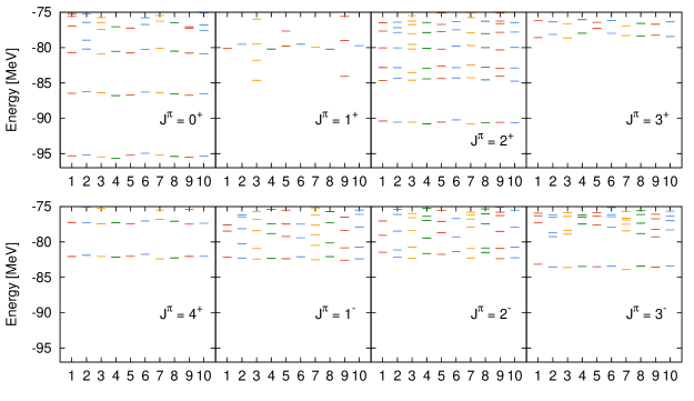
Figure 2: Energy levels of ¹²C nucleus for $J^{\pi}=0^{+},1^{+},2^{+},3^{+},4^{+},1^{-},2^{-}$ and $3^{-}$. Calculations employing ten different sets of SDs are shown. See the text for details.

III.2 Energy levels

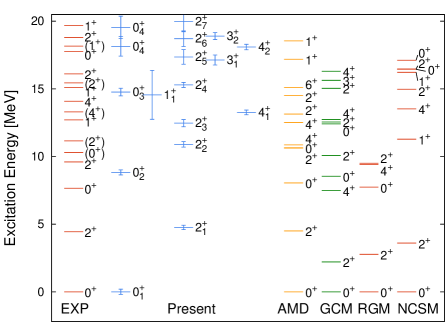
Figure 3: Excitation energies of positive parity are shown. The energies are obtained by averaging over ten configurations. The standard deviations of the energies are also shown by error bars. We also show the results of AMD Kanada-En’yo (2007), GCM Uegaki et al. (1979), RGM Kamimura (1981) and NCSM Navrátil and Ormand (2003). See the text for details.

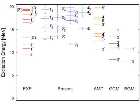
Figure 4: Excitation energies of negative parity states. The same explanation as that in Fig. 3 applies to others.

We show calculated excitation spectra of even and odd parities in Figs. 3 and 4, respectively. In the figures, energies averaged over ten sets are shown with error bars as the standard deviation. Our calculated results are compared with measurements Ajzenberg-Selove (1990); Zimmerman et al. (2011); Itoh et al. (2011); Freer et al. (2012, 2011) and other theories, AMD Kanada-En’yo (2007), GCM Uegaki et al. (1979), RGM Kamimura (1981), and NCSM Navrátil and Ormand (2003).

In the Skyrme-HF calculation, the binding energy of ¹²C is 90.6 MeV, in reasonable agreement with the measured value, 92.2 MeV. In our configuration mixing calculation, the correlation energy is $4.7\pm 0.2$ MeV. The ground-state energy including the correlation is $95.3\pm 0.2$MeV, slightly lower than the measured value.

Calculated excitation energies of the ground-state rotational band are in good agreement with measurements. In the nice reproduction of the rotational energy levels, the configuration mixing is essential since the ground state solution in the HF calculation is spherical for ¹²C with the SLy4 interaction. The excitation energy of $2_{1}^{+}$ state is well reproduced by the present calculation, AMD, and NCSM. However, microscopic $\alpha$ cluster models (GCM and RGM) provide too low excitation energies. The former models (present, AMD, and NCSM) take into account the spin-orbit interaction, while it is not included in the latter (GCM and RGM) in which existence of the three $\alpha$ clusters are assumed. This suggests that a proper inclusion of the spin-orbit interaction is important for the good description of the ground rotational band.

The $0_{2}^{+}$ state, known as the Hoyle state, has been attracting much attention recently since it has been shown that this state may be understood as the Bose condensed state of three $\alpha$ particles Funaki et al. (2003). Our calculation gives a reasonable description for this state, although the excitation energy is slightly overestimated by about 1 MeV. Properties of this state will be discussed in the following subsections. Although recent ab-initio approaches have been successful for the ground-state rotational band, a satisfactory description for the $0_{2}^{+}$ state has not yet been made. For example, the NCSM cannot describe this state adequately Navrátil and Ormand (2003). Recently, attempts of ab-initio description for this state have been undertaken by several groups. A nuclear lattice calculation for this state has been reported in Ref. Epelbaum et al. (2011).

Recently, a new $2^{+}$ state has been found experimentally at $9.6\pm 0.1$ MeV excitation energy with a width of $0.6\pm 0.1$ MeV Freer et al. (2009); Zimmerman et al. (2011) This state was interpreted as the excited state built on the $0_{2}^{+}$ state. In our calculation, two $2^{+}$ states, $2_{2}^{+}$ and $2_{3}^{+}$, appear just above the $0_{2}^{+}$ state. However, as we discuss in Sec. III.3, these two states, $2_{2}^{+}$ and $2_{3}^{+}$, in the present calculation, seem not to correspond to rotationally excited state of the Hoyle state.

In Fig. 3, three states, $0_{3}^{+}$, $2_{4}^{+}$, and $4_{2}^{+}$, follow a rotational energy sequence. Small standard deviations of the energies of these states indicate the reliability of the calculation. As will be discussed in Sec. III.3, these states are connected by strong $B(E2)$ transitions. In Sec. III.6, we will show that this band corresponds to a three-$\alpha$ linear-chain state.

For the negative parity states, we have obtained solid results only for the lowest energy state for each $J^{\pi}$ sector (Sec. III.1). Our calculation reproduces the measured order of the three states, $3_{1}^{-}$, $1_{1}^{-}$ and $2_{1}^{-}$. However, the excitation energies are higher than the measurements by 2-3 MeV.

We would like to stress that our calculation includes no empirical parameter specific to the system, ¹²C nucleus. We employ the SLy4 parameter set which is determined to reproduce nuclear properties of whole mass region. This is in contrast to cluster model calculations where nuclear force parameters are often adjusted for respective systems. We also do not employ any effective charges in evaluating the transition matrix elements shown below.

Finally we mention how the calculated energy levels depend on the choice of the Skyrme interaction. In Fig. 5, we show the excitation energies of positive parity states with different parameter sets of the Skyrme interaction, SLy4, SkM*, and SIII. The same set of SDs (No. 1 in Fig. 2) is employed in all calculations. The correlation energies in the ground state are shown as well inside the parentheses. The comparison shows that basic features of the spectra do not depend much on the choice of the Skyrme parameters. For example, the ground rotational band is described reasonably by all three parameter sets. The position of $0_{2}^{+}$ state does not change much. There appear rotational band in three calculations starting with $0_{3}^{+}$ state. We thus conclude that the excitation energies are not sensitive to the choice of the Skyrme parameters for almost all the states below 15 MeV.

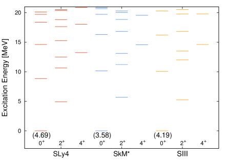
Figure 5: Energy levels of positive parity employing different parameter sets of Skyrme force, SLy4, SkM* and SIII. The number in parentheses is the correlation energy in the ground state, $E_{\rm HF}-E_{\rm gs}$, in unit of MeV. In the calculation, the same set of SDs is employed.

III.3 Transition strength

Transitions	Exp	Cal	AMD	GCM	RGM	NCSM	THSR
$B(E2;2_{1}^{+}\rightarrow 0_{1}^{+})$	7.6$\pm$0.4	8.6 $\pm$0.2	8.5	8.0	9.3	4.146	9.06
$B(E2;4_{1}^{+}\rightarrow 2_{1}^{+})$		13.4$\pm$0.5	16				10.73
$B(E2;0_{2}^{+}\rightarrow 2_{1}^{+})$	13$\pm$2	13.6$\pm$1.2	25.5	3.5	5.5		4.71
$B(E2;2_{2}^{+}\rightarrow 0_{2}^{+})$		0.17$\pm$0.23
$B(E2;2_{3}^{+}\rightarrow 0_{2}^{+})$		5.9$\pm$0.7
$B(E2;2_{4}^{+}\rightarrow 0_{2}^{+})$		10$\pm$1	100∗				391
$B(E2;2_{4}^{+}\rightarrow 0_{3}^{+})$		91$\pm$13	310∗
$B(E2;4_{2}^{+}\rightarrow 2_{4}^{+})$		131$\pm$22	600∗
$B(E3;3_{1}^{-}\rightarrow 0_{1}^{+})$	107$\pm$14	77$\pm$4		99	124
$M(E0;0_{1}^{+}\rightarrow 0_{2}^{+})$	5.4$\pm$0.2	4.5$\pm$0.2	6.7	6.6	6.7		6.50

Table 1: $B(E2)$, $B(E3)$ and $M(E0)$ values of ¹²C in units of $e^{2}{\rm fm}^{4}$, $e^{2}{\rm fm}^{6}$ and $e{\rm fm}^{2}$ respectively. Experimental and calculated values are shown in the first and second column, respectively. For comparison, results of the AMDKanada-En’yo (2007), GCMUegaki et al. (1979), RGMKamimura (1981), NCSMNavrátil and Ormand (2003), and THSR are shown. Values in THSR are calculated with the same model as Ref. Funaki et al. (2003). The values indicated by * correspond to $B(E2;2_{2}^{+}\rightarrow 0_{2}^{+})$, $B(E2;2_{2}^{+}\rightarrow 0_{3}^{+})$ and $B(E2;4_{2}^{+}\rightarrow 2_{2}^{+})$ in Ref. Kanada-En’yo (2007). See text for details.

Calculated $B(E2)$, $B(E3)$, and $M(E0)$ values, the average values and the standard deviations, are shown in Table 1. In our calculated values, we do not employ any effective charges. The $B(E2)$ transition strength between $2_{1}^{+}$ and $0_{1}^{+}$ states is well reproduced by our calculation. It is also consistent with results of other theories. The standard deviation is small, about 3%, indicating that our calculated value is well converged.

The $B(E2)$ transition between $0_{2}^{+}$ and $2_{1}^{+}$ is calculated as $13.6\pm 1.2e^{2}{\rm fm}^{4}$, which is in excellent agreement with the measured value, $13\pm 2e^{2}{\rm fm}^{4}$. Other theories fail to reproduce the rate. In Ref. Kanada-En’yo (2007), it is argued that this transition strength is sensitive to the $\alpha$-breaking effect. A good reproduction of this transition strength by our calculation indicates that our calculation reasonably takes account of the $\alpha$-cluster components in the states.

As mentioned in Sec. III.2, there appear two $2^{+}$ states, $2_{2}^{+}$ and $2_{3}^{+}$, above the $0_{2}^{+}$ state in our calculation. These states might correspond to the $2^{+}$ state at 9.6 MeV which was discovered recently Freer et al. (2009); Zimmerman et al. (2011). It was suggested to be a candidate of rotationally excited state built on the $0_{2}^{+}$ state. In the present calculation, however, the $B(E2)$ transition strength between $0_{2}^{+}$ and $2_{2}^{+}$ states is small as seen in Table 1. The rate between $0_{2}^{+}$ and $2_{3}^{+}$ states is also not very large. The $B(E2)$ rate from $0_{2}^{+}$ state is the largest for $2_{4}^{+}$ state which is regarded as rotationally excited state built on the $0_{3}^{+}$ state, as will be mentioned below. These observations suggest that the $2_{2}^{+}$ and $2_{3}^{+}$ states in the present calculation do not correspond to a rotationally excited state on the $0_{2}^{+}$ state.

As we discussed in Sec. III.2, the states of $0_{3}^{+}$, $2_{4}^{+}$, and $4_{2}^{+}$ follow the rotational energy sequence. The calculated transition strengths of $B(E2;2_{4}^{+}\rightarrow 0_{3}^{+})$ and $B(E2;4_{2}^{+}\rightarrow 2_{4}^{+})$ are very large. These results strongly support that these states indeed constitute a rotational band. In Sec. III.6, we will see that this band is dominated by the three-$\alpha$ linear-chain structure.

In the AMD calculation Kanada-En’yo (2007), intense $B(E2)$ values are reported in the transitions among $0_{3}^{+}$, $2_{2}^{+}$, and $4_{2}^{+}$ states. Since the states corresponding to $2_{2}^{+}$ and $2_{3}^{+}$ in our calculation seem not to be present in the AMD calculation, we put these $B(E2)$ values by AMD at the places of $B(E2;2_{4}^{+}\rightarrow 0_{3}^{+})$ and $B(E2;4_{2}^{+}\rightarrow 2_{4}^{+})$ in Table 1. In Ref. Kanada-En’yo (2007), these states are considered as the three-$\alpha$ linear-chain states. The large $B(E2)$ values are qualitatively consistent with our result, though the absolute magnitudes of the transition strengths are much smaller in the present calculation.

For negative-parity states, experimental data for $B(E3;3_{1}^{-}\rightarrow 0_{1}^{+})$ are available. The present calculation gives $77\pm 4e^{2}{\rm fm}^{6}$, which is slightly smaller than the measured value, $107\pm 14e^{2}{\rm fm}^{6}$.

Finally, we discuss the $M(E0)$ transition strength between $0_{2}^{+}$ and $0_{1}^{+}$ states. In the studies by cluster models, it has been argued that the magnitude of this transition strength reflects the spatial extension of the $0_{2}^{+}$ state Yamada et al. (2008). Our calculated value, $4.5\pm 0.2e{\rm fm}^{2}$, is slightly smaller than the measured value, $5.4\pm 0.2e{\rm fm}^{2}$. In contrast, microscopic cluster models and AMD have reported an opposite feature, slightly larger values, $6.6-6.7$ $e$ fm², than measurementUegaki et al. (1979); Kamimura (1981); Kanada-En’yo (2007). Experimentally measured value, $5.4\pm 0.2e{\rm fm}^{2}$ Ajzenberg-Selove (1990), is located between our result and those of the other calculations.

III.4 Radii

We next examine root-mean-square (rms) radii of the ground and excited states. Since our wave function does not allow an exact separation of the center-of-mass motion from the internal one, we estimate an approximate correction for the radius due to the center-of-mass motion, and subtract it from the calculated values. We assume a harmonic oscillator motion for the center-of-mass with the oscillator constant given by $\hbar\omega=41A^{-1/3}=17.9$ MeV. The value of the correction in this model is estimated to be 0.07 fm in the harmonic oscillator shell model. The calculated radii after the correction are shown in Table 2.

Our calculated value in the ground state is $2.52\pm 0.01$ fm. This value is somewhat larger than the measured value, $2.31\pm 0.02$ fm. In the HF calculation, the radius is given by $2.44$ fm. Our configuration mixing calculation, therefore, slightly increases the radius. Comparing with other theories, our value is larger than those of GCM and FMD, and is comparable to the value of AMD.

For the $2_{1}^{+}$ state, our calculated radius is slightly larger than that of the ground state. Other theories report almost the same or slightly larger radius for this state.

For the $0_{2}^{+}$ state, we find a significant difference between the present calculation and the others. Our calculated radius is $2.73\pm 0.02$ fm, which is larger than the radius in the ground state. However, this is much smaller than the other calculations which give more than 3 fm Kanada-En’yo (2007); Uegaki et al. (1979); Kamimura (1981); Chernykh et al. (2007); Funaki et al. (2003). In the recent AMD+GCM calculation Suhara and Kanada-En’yo (2010), the radius of 2.9 fm was reported, similar to ours. It has been found that the radius of the $0_{2}^{+}$ state is quite sensitive to the spin-orbit interaction used in the AMD calculation Suhara and Kanada-En’yo (2013). The radius of the $0_{2}^{+}$ state decreases as the strength of the spin-orbit interaction increases. This dependence is understood as follows Suhara and Kanada-En’yo (2013). If the strength of the spin-orbit interaction is weak, the ground state wave function contains substantial amount of the three-$\alpha$-cluster component. Then, the $0_{2}^{+}$ wave function, which is dominated by dilute three-$\alpha$ components, spatially expands to ensure the orthogonalization to the ground state. As the spin-orbit interaction increases, the three-$\alpha$ component decreases in the ground state, which allows $0_{2}^{+}$ wave function to include more compact three-$\alpha$ structure. This change results in decrease of the radius in $0_{2}^{+}$ state. This mechanism may explain the discrepancy in the $0_{2}^{+}$ radius between our calculation and other theories. It should be noted again that our calculated value for the $M(E0)$ transition strength is smaller than the calculated values by other theories. We also note that an indirect measurement of radius for the $0_{2}^{+}$ state using diffraction inelastic scattering Danilov et al. (2009) was reported, giving $2.89\pm 0.04$ fm.

For the $0_{3}^{+}$ state, our calculated radius is $3.20\pm 0.05$ fm, which is much larger than the radii of $0_{1}^{+}$ and $0_{2}^{+}$ states. This is again smaller than those by other models listed in Table.2, while it is similar to the value (3.26 fm) in Ref. Suhara and Kanada-En’yo (2010).

$J^{\pi}$	EXP	present	AMD	FMD	GCM	RGM	THSR
$0_{1}^{+}$	2.31(2)	2.52$\pm$0.01	2.53	2.39	2.40	2.40	2.39
$0_{2}^{+}$		2.73$\pm$0.02	3.27	3.38	3.40	3.47	3.80
$0_{3}^{+}$		3.20$\pm$0.05	3.98	4.62	3.52
$2_{1}^{+}$		2.60$\pm$0.01	2.66	2.50	2.36	2.38	2.36

Table 2: Mass rms radii of the ground and excited states of ¹²C. The experimental data is taken from Ref. Ozawa et al. (2001). For comparison, we show the results of AMD Kanada-En’yo (2007), FMD Chernykh et al. (2007), GCM Uegaki et al. (1979) , RGM Kamimura (1981) and THSR.

III.5 Charge form factors

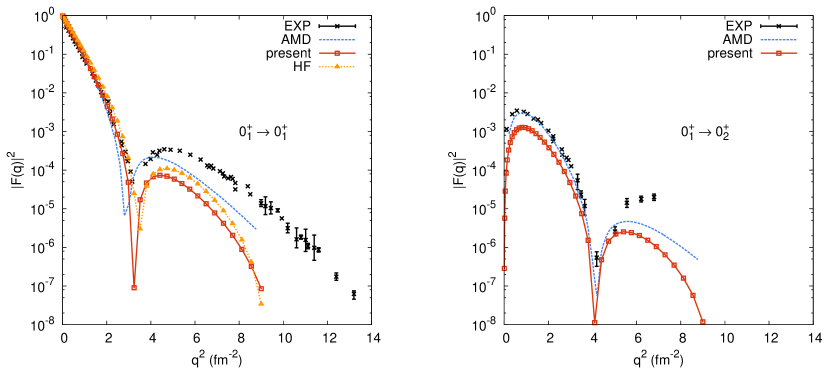
Figure 6: Squared elastic form factor for the ground state (left) and $0_{1}^{+}\rightarrow 0_{2}^{+}$ inelastic form factor (right) are shown. Our calculated results are compared with the HF calculation with a single SD, measurements Sick and McCarthy (1970); Nakada et al. (1971a, b); Strehl and Schucan (1968) and the AMD calculation Kanada-En’yo (2009). Here, the result of the first set of SDs in Fig. 2 is used.

A charge form factor from the initial state $\big{|}J_{i},M_{i}\big{>}$ to the final state $\big{|}J_{f},M_{f}\big{>}$ is defined as follows,

$$|F_{J_{i}\rightarrow J_{f}}(q^{2})|^{2} =\frac{1}{Z}\frac{1}{2J_{i}+1}$$ (21)

$$\times\sum_{M_{i}M_{j}}\big{|}\big{<}J_{f}M_{f}|\sum_{k}\frac{1+\tau_{z}(k)}{2}e^{i\vec{q}\cdot\vec{r}_{k}}|J_{i}M_{i}\big{>}\big{|}^{2}$$

$$\times F_{p}^{2}(q^{2})\times F_{\rm cm}^{2}(q^{2}),$$

where $Z$ is the proton number and $\vec{q}$ is the transferred momentum. $F_{p}(q^{2})$ is a correction factor for the proton size for which we employ $F_{p}(q^{2})={\rm exp}(-a_{p}^{2}q^{2}/6)$ with $a_{p}=0.831$ fm. To correct the center-of-mass motion, we simply assume that the center-of-mass motion is separated and described by the harmonic oscillator wave function of the same oscillator constant, $\hbar\omega=41A^{-1/3}$ MeV, for both initial and final states. Thus, this leads to $F_{\rm cm}^{2}(q^{2})=\exp(q^{2}b^{2}/2A)$ with $b=1.66$ fm.

In Fig. 6, we show charge form factors for the elastic (left) and inelastic $0_{1}^{+}\rightarrow 0_{2}^{+}$ (right) processes. Red solid curves show our results, blue dashed curves show the results of AMD calculation Kanada-En’yo (2009), and crosses with error bars show experimental results Sick and McCarthy (1970); Nakada et al. (1971a, b); Strehl and Schucan (1968). For the elastic form factor, we also show that of Skyrme HF solution in the ground state.

In the small momentum transfer region $q^{2}<2$ fm^-2, the elastic form factor is well reproduced by the calculation. For $q^{2}>2$ fm^-2, our calculation underestimates the form factor, though position of the dip at around 3 fm^-2 is reproduced well. The inelastic form factor for $0_{1}^{+}\rightarrow 0_{2}^{+}$ transition is underestimated for a whole momentum transfer region. The position of the dip at around 4 fm^-2 is reproduced well.

We show results by the AMD calculation. They are in better agreement with measured values, although the dip position in the elastic form factor is located at somewhat smaller $q^{2}$ value. Microscopic cluster calculations also reproduce the form factors well Uegaki et al. (1979); Kamimura (1981).

The underestimation of the elastic form factor at large $q^{2}$ value indicates that the density in our calculation lacks high momentum component. Since the HF solution gives a better description for the form factor at high momentum, the superposition of a number of Slater determinants turns out to increase the diffuseness in the nuclear surface, making the density distribution function $\rho(r)$ smoother. As for the underestimation in the inelastic form factor of $0_{1}^{+}\rightarrow 0_{2}^{+}$ transition, a possible reason is the difference in the character of the wave functions between the ground and $0_{2}^{+}$ states. As we discussed in the radii, a rather small radius of $0_{2}^{+}$ state in our calculation may indicate a small fraction of three-alpha component in the ground state. The inelastic form factor may be reduced if the correlation structures are different between two states. It has been argued that the magnitude of this form factor at small $q^{2}$ is quite sensitive to the radius of the $0_{2}^{+}$ state Funaki et al. (2006): the magnitude of the form factor at small $q^{2}$ reduces as the radius of the $0_{2}^{+}$ state increases. Our result here is opposite, however. The radius of $0_{2}^{+}$ state in our calculation is smaller than those by cluster models, and the magnitude of the inelastic form factor is also small.

III.6 Analysis for wave functions

In order to clarify what kinds of correlations are included in the wave function after configuration mixing, $\Psi_{n}^{J\pi}$, we calculate the overlap between the energy eigenstate and the projected single SD state,

$$P_{n}^{J\pi,iK} = \frac{\Big{|}\big{<}\Phi_{i}\big{|}\hat{P}^{J\dagger}_{MK}\hat{P}^{\pi}|\Psi^{J\pi}_{n}\big{>}\Big{|}^{2}}{\big{|}\big{<}\Phi_{i}\big{|}\hat{P}^{J}_{KK}\hat{P}^{\pi}\big{|}\Phi_{i}\big{>}\big{|}}$$

$$= \Bigg{|}\sum_{j\nu}f^{J\pi,n}_{j\nu}\frac{1}{\sqrt{e^{J\pi}_{j\nu}}}\sum_{K^{\prime}}v^{J\pi,j\nu}_{K^{\prime}}\frac{\big{<}\Phi_{i}\big{|}\hat{P}^{J}_{KK^{\prime}}\hat{P}^{\pi}\big{|}\Phi_{j}\big{>}}{\sqrt{\big{<}\Phi_{i}\big{|}\hat{P}^{J}_{KK}\hat{P}^{\pi}\big{|}\Phi_{i}\big{>}}}\Bigg{|}^{2},$$

and find the SDs which have large overlap values with $\Psi_{n}^{J\pi}$. We show density distributions of the SDs to visualize the correlations included.

In the following, we use the sequential number of the SDs which we assigned in Sec. II.1, using the result of the first set of SDs in Fig. 2. We also show the $K$ quantum number of the SD and the value of the overlap, $P_{n}^{J\pi,iK}$, in Eq. (LABEL:e:overlap).

III.6.1 The ground rotational band

$0^{+}_{1}$			$2^{+}_{1}$			$4^{+}_{1}$
SD	$K^{\pi}$	%	SD	$K^{\pi}$	%	SD	$K^{\pi}$	%
15	$0^{+}$	90.38	4	$0^{+}$	89.36	4	$0^{+}$	88.60
7	$0^{+}$	87.44	15	$0^{+}$	88.51	15	$0^{+}$	81.02
8	$0^{+}$	84.78	29	$0^{+}$	82.44	29	$0^{+}$	76.86
31	$0^{+}$	84.75	2	$0^{+}$	76.47	7	$0^{+}$	76.60
2	$0^{+}$	81.69	7	$0^{+}$	75.21	29	$1^{+}$	72.63
42	$0^{+}$	80.10	48	$0^{+}$	72.63	15	$1^{+}$	70.60
24	$0^{+}$	80.05	47	$0^{+}$	65.76	3	$0^{+}$	70.46
4	$0^{+}$	79.17	8	$0^{+}$	64.22	47	$0^{+}$	70.28
16	$0^{+}$	78.71	10	$1^{+}$	63.85	48	$0^{+}$	69.85
35	$0^{+}$	77.30	44	$1^{+}$	63.63	2	$0^{+}$	69.66

Table 3: The sequential number, the $K$-value, and the squared overlap value are shown for the SDs which dominate in the wave function of the ground rotational band.

In Table 3, we show the sequential number of the SDs which have large overlap values with the wave function of the ground rotational band, $0_{1}^{+}$, $2_{1}^{+}$, and $4_{1}^{+}$. The overlap values $P_{n}^{J\pi,iK}$ defined by Eq. (LABEL:e:overlap) and $K$ values are shown as well. Since the SDs are non-orthogonal, the sum of the overlap values is not equal to but much larger than unity.

In the ground state $0_{1}^{+}$, the 15th SD has the largest overlap, showing 90% for the overlap value. In $2_{1}^{+}$ and $4_{1}^{+}$ states, the 4th SD is the largest component and the 15th SD is the second largest. To illustrate the nuclear shape of these two SDs, we show contour plots of density distributions of the SDs in the yz, zx, and xy planes in Fig. 7. As seen from the figure, they both show oblate deformed shapes.

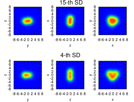
Figure 7: Contour plots of the density distributions of the 15th and the 4th SDs, which are the major components of the ground state rotational band.

The self-consistent HF solution is assigned to the first SD (number 1). We should note that it does not appear in the top ten components of the ground state. Its overlap value with $0_{1}^{+}$ is about 70%. For ¹²C, the self-consistent HF solution with the SLy4 interaction is spherical with $p_{3/2}$ closed shell configuration. The spherical solution cannot describe the rotational band observed in the measurement. As shown in Fig. 3 and Table 1, our calculation accurately reproduces the energy levels and the $B(E2)$ transitions among the states of the ground rotational band. This good reproduction is achieved by a superposition of SDs of deformed shapes.

III.6.2 Negative-parity states

In Table 4, we show sequential numbers of the SD which have large overlap values with the wave function of the negative parity states, $3_{1}^{-}$, $1_{1}^{-}$, and $2_{1}^{-}$. We find the 4th SD, which appears in the ground rotational band, also dominates in the negative parity states. Other SDs which dominate in the negative-parity states are 21, 29, and 47.

We show density distributions of these three SDs in Fig. 8. All of these SDs have similar oblate shapes with three-$\alpha$-like structure. Close look at the densities reveals that the 4th and the 29th SDs have a compact configuration, while the 21th and the 47th SDs show spatially more extended three-$\alpha$ configurations forming an obtuse-angled triangle.

$1^{-}_{1}$			$2^{-}_{1}$			$3^{-}_{1}$			$4^{-}_{1}$
SD	$K^{\pi}$	%	SD	$K^{\pi}$	%	SD	$K^{\pi}$	%	SD	$K^{\pi}$	%
4	$1^{-}$	76.80	21	$1^{-}$	76.50	29	$3^{-}$	81.34	29	$3^{-}$	79.34
47	$1^{-}$	76.35	4	$1^{-}$	75.36	4	$3^{-}$	81.10	47	$3^{-}$	77.26
18	$1^{-}$	75.28	47	$1^{-}$	71.96	47	$3^{-}$	76.17	4	$3^{-}$	76.43
21	$1^{-}$	75.26	22	$1^{-}$	70.24	15	$3^{-}$	66.77	25	$2^{-}$	66.05
22	$1^{-}$	74.03	18	$1^{-}$	69.73	21	$3^{-}$	63.91	41	$3^{-}$	64.37
29	$1^{-}$	68.00	29	$1^{-}$	69.72	3	$1^{-}$	63.63	3	$3^{-}$	60.82
11	$1^{-}$	67.24	11	$1^{-}$	61.80	48	$3^{-}$	61.51	5	$2^{-}$	60.20
25	$1^{-}$	59.97	48	$1^{-}$	55.10	9	$3^{-}$	60.52	9	$3^{-}$	58.79
46	$1^{-}$	57.62	46	$1^{-}$	54.17	41	$1^{-}$	55.94	48	$3^{-}$	56.95
33	$1^{-}$	57.27	33	$1^{-}$	53.68	33	$3^{-}$	54.83	21	$1^{-}$	55.25

Table 4: The sequential number, the $K$-value, and the squared overlap value are shown for the SDs which dominate in the wave function of the negative parity states $1_{1}^{-}$, $2_{1}^{-}$, $3_{1}^{-}$ and $4_{1}^{-}$.

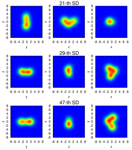
Figure 8: Contour plots of the density distributions of the 21th, 29th, and 47th SDs, which are major components of the negative parity states, $1^{-}_{1}$, $2^{-}_{1}$, $3^{-}_{1}$ and $4^{-}_{1}$.

III.6.3 $0_{2}^{+}$, $2_{2}^{+}$ and $2_{3}^{+}$ states

In Table 5, we show sequential numbers of the SDs which have large overlap values with the wave function of the states, $0_{2}^{+}$, $2_{2}^{+}$ and $2_{3}^{+}$.

We first examine the Hoyle state, $0_{2}^{+}$. Compared with the cases of the ground rotational band and the negative-parity states, the maximum value of the overlap is rather small, less than 50%. This indicates that the superposition of a large number of SDs is essential to describe the $0_{2}^{+}$ state. This is consistent with the cluster-model calculations Uegaki et al. (1979); Kamimura (1981) and the picture of the $\alpha$ condensed state for the $0_{2}^{+}$ state Funaki et al. (2003).

$0^{+}_{2}$			$2^{+}_{2}$			$2^{+}_{3}$
SD	$K^{\pi}$	%	SD	$K^{\pi}$	%	SD	$K^{\pi}$	%
9	$0^{+}$	46.26	16	$2^{+}$	74.07	15	$2^{+}$	50.05
28	$0^{+}$	44.66	35	$0^{+}$	58.22	7	$2^{+}$	40.80
3	$0^{+}$	41.21	43	$0^{+}$	56.18	8	$2^{+}$	40.29
5	$0^{+}$	39.44	42	$0^{+}$	56.00	31	$0^{+}$	39.33
33	$0^{+}$	38.91	31	$2^{+}$	55.69	16	$0^{+}$	31.33
11	$0^{+}$	35.96	7	$1^{+}$	53.55	32	$0^{+}$	22.94
47	$0^{+}$	35.25	32	$2^{+}$	51.61	43	$2^{+}$	21.80
26	$0^{+}$	33.97	49	$0^{+}$	41.33	10	$2^{+}$	20.14
45	$0^{+}$	33.27	36	$2^{+}$	41.02	35	$2^{+}$	19.20
41	$0^{+}$	32.30	43	$1^{+}$	36.06	4	$2^{+}$	18.81

Table 5: The sequential number, the $K$-value, and the squared overlap value are shown for the SDs which dominate in the wave function of the $0_{2}^{+}$m $2_{2}^{+}$ and $2_{3}^{+}$.

We show in Fig. 9 the density distributions of the SDs which have the largest and next largest overlaps with the $0_{2}^{+}$ state, namely, the 9th and the 28th SDs. These SDs have a well developed cluster structures of three $\alpha$-particles.

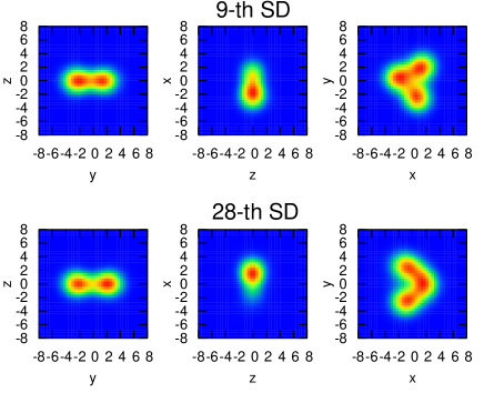
Figure 9: Contour plots of the density distributions of the 9th and the 28th SDs, which are major components in the $0_{2}^{+}$ state.

Regarding the $2_{2}^{+}$ and the $2_{3}^{+}$ states, we find that a number of configurations contribute to these states, as in the case of $0_{2}^{+}$ state. The SDs in $2_{2}^{+}$ and $2_{3}^{+}$ are more or less similar. However, they are very different from those in the $0_{2}^{+}$ state. This is consistent with our observation that the $B(E2)$ transition strengths between $0_{2}^{+}$ and $2_{2}^{+}$ states, and between $0_{2}^{+}$ and $2_{3}^{+}$ states are rather small (see Sec. III.3).

III.6.4 Linear-chain states

$0^{+}_{3}$			$2^{+}_{4}$			$4^{+}_{2}$
SD	$K^{\pi}$	%	SD	$K^{\pi}$	%	SD	$K^{\pi}$	%
30	$0^{+}$	70.13	40	$0^{+}$	78.31	40	$0^{+}$	75.26
40	$0^{+}$	66.70	30	$0^{+}$	72.35	30	$0^{+}$	75.18
19	$0^{+}$	65.11	19	$0^{+}$	71.33	18	$0^{+}$	65.74
20	$0^{+}$	41.88	18	$0^{+}$	67.69	19	$0^{+}$	62.44
23	$0^{+}$	38.47	11	$0^{+}$	59.29	34	$0^{+}$	43.14
18	$0^{+}$	38.02	23	$0^{+}$	57.94	20	$0^{+}$	43.05
14	$0^{+}$	37.56	12	$0^{+}$	47.82	11	$1^{+}$	41.81
12	$0^{+}$	37.23	34	$0^{+}$	47.07	23	$0^{+}$	41.19
11	$0^{+}$	25.46	22	$0^{+}$	39.24	14	$0^{+}$	40.48
22	$0^{+}$	16.63	20	$0^{+}$	39.15	11	$0^{+}$	39.13

Table 6: The sequential number, the $K$-value, and the squared overlap value are shown for the SDs which dominate in the wave function of the $0_{3}^{+}$m $2_{4}^{+}$ and $4_{2}^{+}$..

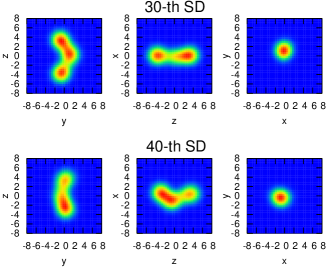
Figure 10: Contour plots of the density distributions of the 30th and the 40th SDs, which are the major components of the $0_{3}^{+}$, $2_{4}^{+}$, and $4_{2}^{+}$ states.

As seen in Sec. III.3, $0^{+}_{3}$, $2_{4}^{+}$ and $4_{2}^{+}$ states are connected by the intense $B(E2)$ values. In Table 6, the sequential numbers of the SD which have large overlap values with the wave function of these states are shown. The 30th, the 40th, and the 19th SDs are commonly included in the three states. We show in Fig. 10 the density distributions of the 30th and the 40th SDs. They clearly show a bended linear-chain structure of three $\alpha$ particles.

IV Mixing of Three-alpha Configurations

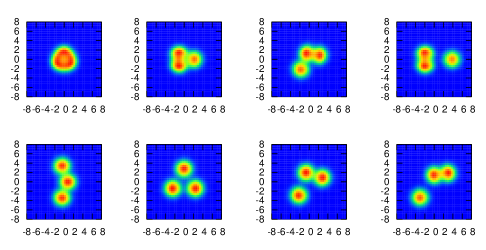
Figure 11: Density distributions of some SDs out of 31 SDs which are used in Ref. Uegaki et al. (1979). Unit of vertical and horizontal axes are fm.

Some of the present results in Sec. III are found to be qualitatively different from those of AMD and microscopic cluster models. For example, the radius of the $0_{2}^{+}$ state is much smaller in our calculation. The charge form factor at large momentum transfer is described much better by other theories than ours. These facts may indicate that the imaginary-time propagation may not sufficiently produce a certain class of $\alpha$-cluster wave functions. In order to check whether explicit inclusion of $\alpha$-cluster configurations bring large changes in the current results, we perform configuration-mixing calculations including the wave functions similar to those employed in the microscopic cluster model of Ref. Uegaki et al. (1979).

The 31 SDs of the $\alpha$-cluster wave functions are used in the GCM calculation in Ref. Uegaki et al. (1979). We place the $\alpha$-particle wave functions at the same positions as those of Ref. Uegaki et al. (1979). In Ref. Uegaki et al. (1979), the single-particle wave functions of the SDs are the Gaussian wave packets. Instead of the Gaussian wave packet, we employ the HF orbitals of the $\alpha$ particles. In Fig. 11, we show density distributions of selected SDs among those 31 SDs.

In Fig. 12, we show excitation spectra from configuration mixing calculations using the 31 SDs. The left panel shows our calculation using SLy4 interaction. The middle panel shows the GCM calculation using Volkov No. I force Uegaki et al. (1979). The results for the ground rotational band are similar to each other. In fact, in both calculations, the moment of inertia is too large. The $0_{2}^{+}$ state appears at around 7 MeV in our calculation, slightly lower than that of Ref. Uegaki et al. (1979).

In the parentheses in Fig. 12, we show the calculated binding energies in the ground state. The absolute values of the binding energies is very different between our calculation and that of Ref. Uegaki et al. (1979). In our calculation using SLy4 interaction, the binding energy is -75.1 MeV and is much smaller than the value shown in Fig. 2. A major part of the difference comes from the spin-orbit interaction which contributes little in the calculation using the alpha-cluster wave functions only.

We next perform a configuration mixing calculation employing both the 50 SDs prepared by the imaginary-time method and the 31 SDs of three-$\alpha$ configuration. In Fig. 13, we compare the three calculations: the configuration mixing calculation using 50 SDs prepared by the imaginary time method (IT), the configuration mixing calculation using 31 SDs of three-$\alpha$ configuration (3$\alpha$), and the configuration mixing calculation using both (IT+3$\alpha$). The calculation labeled by three-$\alpha$ is the same as that shown in the left part of Fig. 13, except that the total energies are plotted here.

After mixing both configurations of the imaginary-time and the three-$\alpha$, we find the results are very close to the calculation using the imaginary-time configurations only. Namely, 31 SDs of the three-$\alpha$ wave functions do not mix with those prepared by the imaginary-time method. This is due to the large energy difference between those two sets of configurations.

In the calculation using configurations generated by the imaginary-time method, the contribution of the spin-orbit interaction to the binding energy is as large as 17 MeV with SLy4. This large energy gain is missing in the pure three-$\alpha$ configurations.

In Table 7, we show the calculated radii and the $M(E0)$ transition strength. Using the 31 SDs of three-$\alpha$ wave functions, our calculation gives large values for both the $0_{1}^{+}$ and $0_{2}^{+}$ states. The radius of the $0_{2}^{+}$ state is 3.31 fm, close to the value by the GCM calculation, 3.4 fm. The $M(E0)$ value is also large, 8.72$e{\rm fm}^{2}$, even larger than the three-$\alpha$ GCM calculation Uegaki et al. (1979). However, in the configuration mixing calculation using both configurations, our calculated values are very close to the calculation using the 50 SDs prepared by the imaginary-time method. This result is consistent with the fact that the energy spectra is very little affected by adding the three-$\alpha$ wave functions.

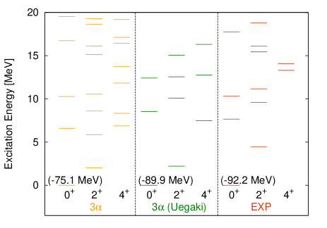
Figure 12: Energy levels of ¹²C employing 3$\alpha$ SDs with Skyrme SLy4 interaction (left), the results of GCM calculation of Ref. Uegaki et al. (1979) (center) and experiments (right).

	EXP	IT	IT + 3$\alpha$	3$\alpha$	3$\alpha$(Uegaki)
radius$(0_{1}^{+})$	2.31$\pm$0.02	2.53	2.54	2.80	2.40
radius$(0_{2}^{+})$		2.76	2.73	3.31	3.40
$M(E0;0_{2}^{+}\rightarrow 0_{1}^{+})$	5.4$\pm$ 0.2	4.57	4.13	8.72	6.6

Table 7: Radii (fm) and $M(E0)$ ($e{\rm fm}^{2}$) calculated in various model spaces. Results of GCM calculation Uegaki et al. (1979) is also shown. See text for details.

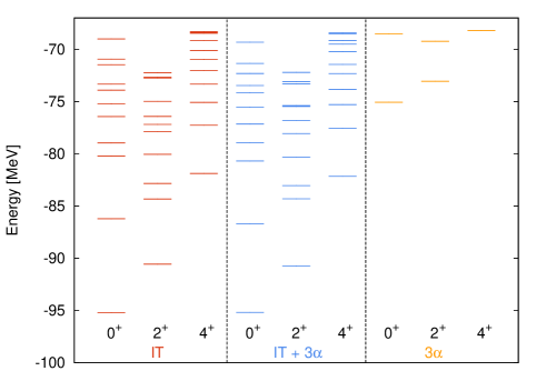
Figure 13: Energy levels of ¹²C in the configuration mixing calculation with the SDs constructed by the imaginary-time evolution (IT), and 3$\alpha$, and all of these configurations (IT+3$\alpha$). See text for details.

V SUMMARY

We have investigated structure of the ¹²C nucleus employing a configuration-mixing approach with Skyrme interaction. In this approach, we first generate a number of Slater determinants using the imaginary-time method Shinohara et al. (2006) starting from initial Slater determinants prepared in a stochastic way. These Slater determinants show various shapes and clustering. They are projected on parity and angular momentum, then, are superposed by the configuration-mixing calculation. We have generated several sets of Slater determinants and compare the results with the different sets, to quantify the reliability of the calculation. A few low-lying states for each parity and angular momentum are well converged with small variance among the different sets of the Slater determinants. This fact indicates that the present calculation provides unique and convergent results for the ground and a few low-lying excited states, once the effective nucleon-nucleon force, the Skyrme interaction in the present calculation, is given.

Our calculation reasonably reproduces the overall features of the structure of ¹²C. The energies and the $B(E2)$ transition strength of the ground state rotational band are well described. The lowest excited states of negative parity, $1^{-}$, $2^{-}$, and $3^{-}$, are also reasonably described, although the excitation energies are slightly too high. The Slater determinants which dominate in these states show three-$\alpha$ structure. Our calculation also reproduces the excitation energy of the Hoyle ($0^{+}_{2}$) state reasonably. This state is found to be described by superposition of many Slater determinants, consistent with the former cluster-model calculations. However, the radius of the $0_{2}^{+}$ state is calculated to be significantly smaller than those. The energy gain associated with the spin-orbit interaction in the present method seems to be responsible for this difference. The three-$\alpha$ liner-chain structure appears at around 15 MeV excitation, forming a rotational band.

The success for the description of ¹²C nucleus reported in this paper clearly shows that the present approach is promising for systematic description of various many-body correlations including clustering in light nuclei.