Orbital entanglement production in Andreev billiards with time-reversal symmetry

Abstract

We study orbital entanglement production in a chaotic cavity connected to four single-channel normal-metal leads and one superconducting lead, assuming the presence of time-reversal symmetry (TRS). The scattered state of two incident electrons is written as the superposition of several two-outgoing quasi-particle states, four of which are orbitally entangled in a left-right bipartition. We calculate numerically the mean value of the squared norm of each scattered state’s component, as functions of the number of channels in the superconducting lead. Its behavior is explained as resulting from the proximity effect. We also study statistically the amount of entanglement carried by each pair of outgoing quasi-particles. When the influence of the superconductor is more intense, the average entanglement is found to be considerably larger than that obtained using normal cavities.

I Introduction

Quantum correlations are in the very heart of quantum physicsEPR and of applications like quantum computing and quantum cryptography.Nielsen The potential of quantum-transport devices to produce and manipulate entanglement has been explored during the last years.Beenakker.school ; nazarov.livro Several of those devices produce entanglement from scattering processes taking place in its components.

Chaotic cavities have been proposed as orbital entanglers.beenakker.emaranhador The cavity is connected to four one-channel normal-metal leads, two at the left and two at the right. An electron leaving the cavity at either the left or the right represents a qubit, and entanglement between two qubits can be studied considering a left-right bipartition. The mean value and the variance of the concurrence, a quantifier of entanglement, were initially calculated in the context of random matrix theory,beenakker.emaranhador followed by more complete statistical analysis.Frustalgia ; gopar Non-ideal contacts have also been considered.chico ; vivo Constraints on entanglement production imposed by the geometry of the device were explored,Sergio-Marcel-normal and it was found that more entangled states are less likely to be produced in general.

Scattering processes in normal-superconducting (NS) hybrid systems are another source of entanglement.Samuelsson(2003) ; chinese.NS Entangled pairs of quasi-particles can be generated after Andreev reflections which take place at the normal-superconductor interface. In the present work, we propose the use of Andreev billiards as orbital entanglers. We study the generation probability of each pair of quasi-particles, and how this quantity and the amount of entanglement are affected by the influence of the superconductor. We find a notable increase in the production of entanglement induced by the proximity effect,mcmillan(1968) when compared to normal cavities. On the other hand, we observe in general a compensation between the amount of entanglement and the probability of producing it.

The paper is organized as follows. In Sec. II we explain how the device is designed, and what is the structure of its scattering matrix. We also write the scattered state as a function of the transmission properties of the system. The mean value of the squared norms of states describing two-outgoing quasi-particles, even those non-entangled, is analyzed in Sec. III. Statistics of concurrence is studied in Sec. IV. We present its full distribution, as well as its mean value and its variance, for different values of the number of open channels in the superconducting lead. We summarize and conclude in Sec. V. Two additional sections are included as appendices. The equations used to perform the numerical simulations are presented in Appendix A, while some analytical considerations about the squared norms of the entangled states appear in Appendix B.

II Design of the device

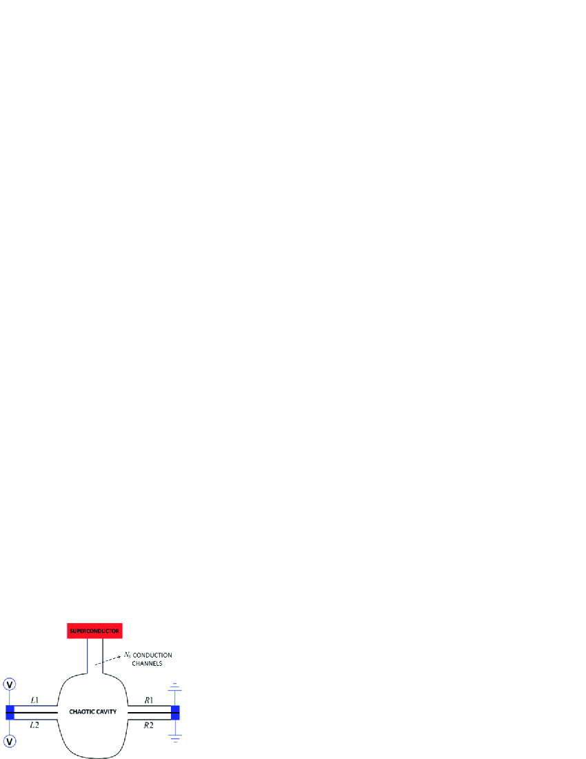
Figure 1: (Color online) A chaotic cavity is attached to four normal leads, denoted by $L_{1}$, $L_{2}$, $R_{1}$ and $R_{2}$, and one floating superconductor lead. Each normal lead has one conduction channel while there are $N_{s}$ open channels in the superconductor lead. A potential $V$ is applied on the left leads and the right leads are grounded.

The setup is represented in Fig. 1. A central chaotic cavity is connected to five leads. Four leads are normal and have only one open conduction channel; they are represented at the left and right sides of the cavity and denoted by $L_{1}$, $L_{2}$, $R_{1}$, and $R_{2}$. A superconducting lead with $N_{s}$ channels is attached to the top of the cavity. A potential $V$ is applied on the left leads and the right leads are grounded. The superconducting lead is floating. Thus an electrical current crosses the device by the normal leads. Specifically, pairs of electrons with energies between the Fermi energy $E_{F}$ and $E_{F}+eV$ enter the cavity from the left leads. It is assumed that the energy of the incident electrons is much smaller than the gap $\Delta$ in the superconductor, i.e. $eV\ll\Delta$. This implies that charge transfer in the NS interface takes place only via Andreev reflection.andreev Since the device has only one superconducting lead, the phase of the superconductor is irrelevant. We also neglect temperature fluctuations.

II.1 Scattering matrix of the system

The potential $V$ is small enough to neglect the dependence on energy of the scattering matrix. We emphasize that this matrix does not belong to any universal class of random matrices. In order to reach universality in the presence of TRS, it would be necessary to attach another superconducting lead to the cavity, with a phase difference of $\pi$.altland(1997) ; melsen(1997) Also the number of open channels in the superconducting lead must be larger than one.brouwer(2000) We focus on a different regime, where proximity effects are important. The scattering matrix will be denoted by $S_{NS}$ and has the following structure:

$$S_{NS}=\left(\begin{array}[]{cc}\hat{r}&\hat{t}^{\prime}\\ \hat{t}&\hat{r}^{\prime}\end{array}\right).$$ (1)

The blocks $\hat{r}$ ($\hat{r}^{\prime}$) and $\hat{t}$ ($\hat{t}^{\prime}$) contain, respectively, the reflection and the transmission amplitudes for quasi-particles coming from the left (right). Each block has its own electron-hole structure, which is indicated with the hat symbol. For example, the matrix $\hat{r}$ is

$$\hat{r}=\left(\begin{array}[]{cc}r^{ee}&r^{eh}\\ r^{he}&r^{hh}\end{array}\right).$$ (2)

On the other hand, each sub-block $r^{\alpha\beta}$ in the last equation is a $2\times 2$ matrix, whose elements are the reflection amplitudes for the leads $L_{1}$ and $L_{2}$. They are given by

$$r^{\alpha\beta}=\left(\begin{array}[]{cc}r^{\alpha\beta}_{11}&r^{\alpha\beta}_{12}\\ r^{\alpha\beta}_{21}&r^{\alpha\beta}_{22}\end{array}\right).$$ (3)

The other blocks of $S_{NS}$ have the same structure. The scattering matrix of the whole system can be expressed as a function of the scattering matrix of the normal cavity,rev.beenakker which belongs to the Circular Orthogonal Ensemble. Equations showing this dependence are presented in Appendix A.

II.2 Scattered state

The scattered state of two incident electrons can be expressed as $|\Psi_{\mathrm{scat}}\rangle=|\Psi_{LL}\rangle+|\Psi_{RR}\rangle+|\Psi_{LR}\rangle$. State $|\Psi_{LL}\rangle$ ($|\Psi_{RR}\rangle$) characterizes two quasi-particles being scattered to the left (right), so is not entangled. One quasi-particle scattered to the left and the other one to the right is represented by the state $|\Psi_{LR}\rangle$. In order to give explicit expressions for these three states, we define the projector matrix

$$\sigma^{\prime}=\mathrm{i}\,\sigma_{y}\otimes\begin{pmatrix}1&0\\ 0&0\end{pmatrix}.$$ (4)

The structure of this matrix accounts for the fact that the incident state is given by two electrons coming from the left. It is also convenient to define the operators $\mathcal{L}^{\alpha}_{j}$ and $\mathcal{R}^{\alpha}_{j}$, which create a quasi-particle of type $\alpha$ going out at the lead $L_{j}$ and $R_{j}$, respectively, with energy $\epsilon$ if $\alpha=e$ and $-\epsilon$ if $\alpha=h$ ($E_{F}<\epsilon<E_{F}+eV$). We also define

$$\hat{\delta}=\hat{r}\sigma^{\prime}\hat{r}^{\,T},$$ (5)

$$\hat{\eta}=\hat{t}\sigma^{\prime}\hat{t}^{\,T},$$ (6)

$$\hat{\gamma}=\hat{r}\sigma^{\prime}\hat{t}^{\,T},$$ (7)

where the superscript “$T$” indicates the transposition operation. Using the above objects, the three states can be expressed in the following way:

$$|\Psi_{LL}\rangle=\frac{1}{2}\sum\limits_{jk;\alpha\beta}{\delta_{jk}^{\alpha\beta}\;\mathcal{L}^{\alpha}_{j}\;\mathcal{L}^{\beta}_{k}\;|0\rangle},$$ (8)

$$|\Psi_{RR}\rangle=\frac{1}{2}\sum\limits_{jk;\alpha\beta}{\eta_{jk}^{\alpha\beta}\;\mathcal{R}^{\alpha}_{j}\;\mathcal{R}^{\beta}_{k}\;|0\rangle},$$ (9)

$$|\Psi_{LR}\rangle=\sum\limits_{jk;\alpha\beta}{\gamma_{jk}^{\alpha\beta}\;\mathcal{L}^{\alpha}_{j}\;\mathcal{R}^{\beta}_{k}\;|0\rangle},$$ (10)

where $|0\rangle$ is the state without electronic excitations. Each term in these sums represents a pair of quasi-particles of types $\alpha$ and $\beta$ getting out at the leads $j$ and $k$. The equations presented in this section are general and do not specify any particular property of the NS system.

III Statistics of the squared norms

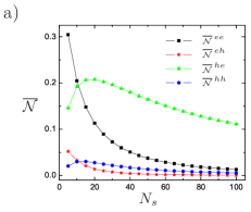
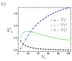
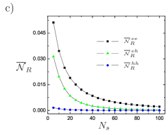
Figure 2: (Color online) Mean values of the squared norms $\mathcal{N}^{\alpha\beta}$, $\mathcal{N}_{L}^{\alpha\beta}$, and $\mathcal{N}_{R}^{\alpha\beta}$ are represented in panels a), b), and c) respectively, for different numbers of open channels in the superconducting lead. $10^{5}$ samples were generated for each value of $N_{s}$.

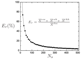
Figure 3: Function $E_{r}$ (in percent) for values of $N_{s}$ varying from $10$ to $500$. Each dot was calculated using $5\times 10^{3}$ random matrices.

In this section we focus on the probability of producing, during a fixed time, a given number of pairs $\alpha$ and $\beta$ being scattered to the left, to the right, or to different sides. This probability is determined by the squared norm of the state which represents each process. Let us denote such squared norms as $\mathcal{N}_{L}^{\alpha\beta}$, $\mathcal{N}_{R}^{\alpha\beta}$, and $\mathcal{N}^{\alpha\beta}$. We are assuming that $\mathcal{N}^{\alpha\beta}$ refers to the quasi-particle $\alpha$ scattered to the left and the other one, $\beta$, to the right. For the other two squared norms there is no distinction between $\alpha,\beta$. Using Eqs. (8)-(10), they are expressed as functions of the transmission properties of the system through the following equations:

$$\mathcal{N}_{L}^{\alpha\beta}=\mathrm{Tr}(\delta^{\alpha\beta}{\delta^{\alpha\beta}}^{\dagger}),$$ (11)

$$\mathcal{N}_{R}^{\alpha\beta}=\mathrm{Tr}(\eta^{\alpha\beta}{\eta^{\alpha\beta}}^{\dagger}),$$ (12)

$$\mathcal{N}^{\alpha\beta}=\mathrm{Tr}(\gamma^{\alpha\beta}{\gamma^{\alpha\beta}}^{\dagger}).$$ (13)

Let us discuss the underlying mechanism behind the influence of proximity effects on transport properties. As the number of open channels in the superconducting lead increases, the probability of incident electrons to undergo an Andreev reflection in the NS interface and thus to be backscattered as holes to the left before “feeling” the chaos of the cavity gets larger. As $N_{s}\rightarrow\infty$ this probability becomes unit, and the device works as if all electrons were Andreev reflected upon arrival at the cavity.brouwer(2000)

A consequence of direct Andreev backscattering is an increased number of holes leaving the cavity at the left, and therefore a decreased transmission of any quasi-particle to the right. This is verified in Fig. 2. As $N_{s}$ gets bigger, $\overline{\mathcal{N}}^{ee}$, $\overline{\mathcal{N}}^{eh}$, $\overline{\mathcal{N}}_{L}^{ee}$, $\overline{\mathcal{N}}_{R}^{ee}$, and $\overline{\mathcal{N}}_{R}^{eh}$ monotonically decrease, because the probability of an electron to be scattered to the left continually decreases. On the other hand, $\overline{\mathcal{N}}^{he}$, $\overline{\mathcal{N}}^{hh}$ and $\overline{\mathcal{N}}_{L}^{eh}$ have a non-monotonic behavior, initially increasing due to direct Andreev backscattering. The quantity $\overline{\mathcal{N}}^{he}$ decreases more slowly than the other squared norms of entangled states because scattering to the right is more probable for electrons than for holes. Furthermore, $\overline{\mathcal{N}}_{L}^{hh}$ ($\overline{\mathcal{N}}_{R}^{hh}$) monotonically increases (decreases), also because of direct Andreev backscattering.

The dominance of $\overline{\mathcal{N}}^{he}$ over the other entangled components can be quantified by

$$E_{r}=\frac{\overline{\mathcal{N}}^{ee}+\;\;\overline{\mathcal{N}}^{eh}+\;\;\overline{\mathcal{N}}^{hh}}{\overline{\mathcal{N}}^{he}}.$$ (14)

The behavior of $E_{r}$ is shown in Fig. 3, where $N_{s}$ runs from $10$ to $500$. Notice that for $N_{s}=500$, the sum of the other components represents less than $5\%$ of $\overline{\mathcal{N}}^{he}$. Although all four kinds of events are rare for large values of $N_{s}$, a setup for detection of entanglement would characterize correlations between one left-outgoing hole and one right-outgoing electron with a small relative error.

Direct Andreev backscattering does not occur if TRS is broken, because a random phase is accumulated during the process and so it is killed after averaging. An implication of this is that in the presence of a magnetic field and for $N_{s}\gg 1$, the statistical distributions of $\mathcal{N}^{\alpha\beta}$ are very similar for any $\alpha$ and $\beta$. We corroborated this observation through numerical simulations (not shown).

IV Statistics of concurrence

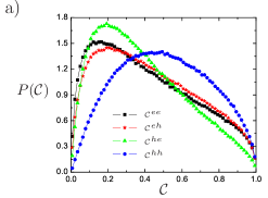
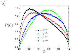
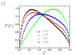
Figure 4: (Color online) Distributions of concurrence are represented for $N_{s}$ equal to a) $5$, b) $25$, and c) 100. Each distribution was made using $10^{6}$ random matrices.

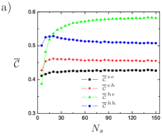
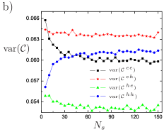
Figure 5: (Color online) a) Mean value and b) variance of the concurrence calculated from $10^{5}$ random matrices for each value of $N_{s}$.

The concurrence of the entangled states is given bywootters ; Beenakker.Hall

$$\mathcal{C}^{\alpha\beta}=2\sqrt{\mathrm{Det}(\gamma^{\alpha\beta}{\gamma^{\alpha\beta}}^{\dagger})}/\mathrm{Tr}(\gamma^{\alpha\beta}{\gamma^{\alpha\beta}}^{\dagger}).$$ (15)

In contrast with the result obtained for a generic normal system,beenakker.emaranhador this expression depends not only on the eigenvalues of the normal scattering matrix, but on its eigenvectors as well. This prevents us from proving the geometric constraint for the squared norm and the concurrence discovered in Ref. Sergio-Marcel-normal, for normal systems, that forces $\mathcal{N}(1+\mathcal{C})<1$. Nevertheless, we have observed in numerical simulations that this constraint seems to remain valid for the considered system. Using Eqs. (7), (15), and taking into account the unitarity of $S_{NS}$, a weaker constraint can be proved,

$$\mathcal{N}^{\alpha\beta}\mathcal{C}^{\alpha\beta}\leq 1/2.$$ (16)

This inequality is not related to specific physical properties of the system, but it is an implication of unitarity and the design of the device.

Fig. 4 shows the distributions of concurrence for $N_{s}=5$, $25$, and $100$. They suggest that all pairs of left-right outgoing quasi-particles are entangled, but none of them is maximally entangled. It is clearly seen that $\mathcal{C}^{he}$ is the quantity most sensitive to the presence of the superconductor. However, variations are small for all the distributions when $N_{s}$ is large, which indicates convergence, as can be observed in Fig. 5 where we show the average value and the variance of the concurrence.

As the number $N_{s}$ increases, there is a remarkable enhancement in the production of entanglement for the hole-electron component: $\overline{\mathcal{C}}^{he}$ reaches values above $0.58$, reflecting a considerable increase compared to the normal case, where $\overline{\mathcal{C}}\approx 0.38$.beenakker.emaranhador Note that the other three components have only slight dependence on $N_{s}$. Moreover, variations of $\mathcal{C}^{he}$ from sample to sample are more concentrated around its mean value than for the other components. The variance of this quantity decreases as $N_{s}$ increases (see Fig. 5b). We found that $\mathrm{var}(\mathcal{C}^{he})$ oscillates around $0.53$ for large $N_{s}$. This value is slightly less than the variance for the other components, as well as those found for a normal cavity.beenakker.emaranhador

V Summary and conclusions

We studied orbital entanglement production in Andreev billiards, assuming time-reversal symmetry in the system. Numerical simulations were performed to statistically analyze the squared norm and the concurrence of states describing a pair of outgoing quasi-particles. The behavior of the squared norm for varying numbers of channels in the superconducting lead was explained as a consequence of Andreev reflection. Even though the norms of the entangled components decrease as the influence of the superconductor is stronger, the squared norm of the state describing one left-outgoing hole and one right-outgoing electron always dominates. In this regime, there is a notable enhance in the amount of entanglement for that state. The mean concurrence reaches values greater than $0.58$, exceeding the value found for a normal cavity.

There exist a general feature in the entanglement production using the geometry studied in this paper and other works.beenakker.emaranhador ; Frustalgia ; gopar ; chico ; vivo ; Sergio-Marcel-normal The profit obtained in the amount of entanglement is, in some way, compensated by a decreased probability of producing the state. In the case of the system under consideration, this tendency is reinforced by the proximity effect.

It is still an open problem to establish a suitable setup for detection of the entanglement carried by each type of outgoing pair of quasi-particles.

Appendix A Equations to perform the numerical simulations

Let’s define the matrix of the normal cavity as

$$S_{0}=\left(\begin{array}[]{cc}r_{0}&t^{\prime}_{0}\\ t_{0}&r^{\prime}_{0}\end{array}\right).$$ (17)

Our numerical simulations are performed through random generations of $S_{0}$, which has dimensions $2N_{s}\times 2N_{s}$. We need to close $N_{s}-4$ conduction channels in the normal side (assuming $N_{s}>4$), which is done introducing a fictitious barrier with very small transparency. Only four channels remain open, one for each normal lead. The scattering matrix for the fictitious connector is given by

$$S_{c}=\left(\begin{array}[]{cc}r_{c}&t^{\prime}_{c}\\ t_{c}&r^{\prime}_{c}\end{array}\right).$$ (18)

We choose $r_{c}=r^{\prime}_{c}$, $t_{c}=t^{\prime}_{c}$, and define

$$r_{c}=\left(\begin{array}[]{cc}\sqrt{\Gamma}I_{4}&0\\ 0&\sqrt{1-\Gamma}I_{N_{s}-4}\end{array}\right),$$ (19)

and

$$t_{c}=\mathrm{i}\left(\begin{array}[]{cc}\sqrt{1-\Gamma}I_{4}&0\\ 0&\sqrt{\Gamma}I_{N_{s}-4}\end{array}\right),$$ (20)

$\Gamma$ being the transparency of the barrier, and $I_{n}$ the $n\times n$ identity matrix.

First, it is necessary to compose $S_{0}$ and $S_{c}$, to obtain the total normal scattering matrix $S_{N}$. This is done using the following equations:

$$r_{N} =r_{c}+t_{c}M_{N}r_{0}t_{c},$$ (21)

$$t_{N} =\mathrm{i}\;t_{0}(I_{n}+r_{c}M_{N}r_{0})t_{c},$$ (22)

$$r^{\prime}_{N} =-r^{\prime}_{0}-t_{0}r_{c}M_{N}t^{\prime}_{0},$$ (23)

$$t^{\prime}_{N} =\mathrm{i}\;t_{c}M_{N}t^{\prime}_{0},$$ (24)

where $M_{N}=(I_{N_{s}}-r_{0}r_{c})^{-1}$. The phase of the superconductor is irrelevant and it can be set equal to zero. Neglecting the energy-dependence, the blocks of $S_{NS}$ in the electron-hole space can be written as rev.beenakker

$$S_{NS}^{ee}=r_{N}-t^{\prime}_{N}(r^{\prime}_{N})^{\ast}M_{e}t_{N},$$ (25)

$$S_{NS}^{eh}=-\mathrm{i}\;(t^{\prime}_{N})^{\ast}M_{e}t_{N},$$ (26)

where $M_{e}=(I_{N_{s}}+r^{\prime}_{N}(r^{\prime}_{N})^{\ast})^{-1}$. On the other hand, $S_{NS}^{\;\alpha\beta}$ is structured as

$$S_{NS}^{\;\alpha\beta}=\left(\begin{array}[]{cc}r^{\alpha\beta}&{t^{\prime}}^{\alpha\beta}\\ t^{\alpha\beta}&{r^{\prime}}^{\alpha\beta}\end{array}\right).$$ (27)

$S_{NS}^{\;eh}$ and $S_{NS}^{\;hh}$ are not necessary to calculate norm and concurrence, because we consider the initial state given by two electrons entering the cavity from the left.

Appendix B Some analytical considerations about $\mathcal{N}^{\alpha\beta}$

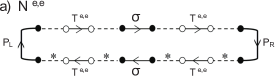
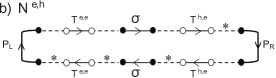
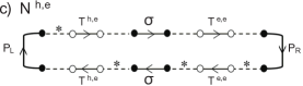
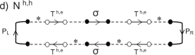
Figure 6: The squared norms of the entangled components are sketched using the symbology of the diagrammatical method for averaging over the unitary group.

We proceed analogously to Ref. Samuelsson(2002), , where a similar device was studied. However, an essential difference is the small numbers of open channels in the normal leads, which requires to take into account all diagrams.

It is convenient to parameterize the scattering matrix of the cavity through the polar decomposition mello-pereira-kumar(1988) ; rev.beenakker

$$S_{0}=\left(\begin{array}[]{cc}v\sqrt{I_{4}-T}v^{T}&v\begin{pmatrix}0&\mathrm{i}\sqrt{T}\end{pmatrix}w^{T}\\ \\ w\begin{pmatrix}0\\ \mathrm{i}\sqrt{T}\end{pmatrix}v^{T}&\;\;w\begin{pmatrix}I_{N_{s}-4}&0\\ 0&\sqrt{I_{4}-T}\end{pmatrix}w^{T}\end{array}\right).$$ (28)

In the above equation $v$ and $w$ have dimensions $4\times 4$ and $N_{s}\times N_{s}$, respectively, and belong to unitary circular ensembles. They account for the isotropy assumption.rev.beenakker On the other hand, $T={\rm diag}(\tau_{L_{1}},\tau_{L_{2}},\tau_{R_{1}},\tau_{R_{2}})$ is a function of the transmission eigenvalues. The eigenvalue $\tau_{L_{j}(R_{j})}$ quantifies the probability that an electron entering from lead $L_{j}$ ($R_{j}$) meets the superconductor before leaving the cavity.

Making $S_{N}=S_{0}$ in Eqs. (25) and (26), and using the polar decomposition, the equations for the squared norms of the entangled components can be written as

$$\mathcal{N}^{ee}=-\mathrm{Tr}\left[P_{L}v\mathcal{T}^{ee}v^{T}\sigma v\mathcal{T}^{ee}v^{T}P_{R}v^{\ast}\mathcal{T}^{ee}v^{\dagger}\sigma v^{\ast}\mathcal{T}^{ee}v^{\dagger}\right],$$ (29)

$$\mathcal{N}^{eh}=-\mathrm{Tr}\left[P_{L}v\mathcal{T}^{ee}v^{T}\sigma v\mathcal{T}^{he}v^{\dagger}P_{R}v\mathcal{T}^{he}v^{\dagger}\sigma v^{\ast}\mathcal{T}^{ee}v^{\dagger}\right],$$ (30)

$$\mathcal{N}^{he}=-\mathrm{Tr}\left[P_{L}v^{\ast}\mathcal{T}^{he}v^{T}\sigma v\mathcal{T}^{ee}v^{T}P_{R}v^{\ast}\mathcal{T}^{ee}v^{\dagger}\sigma v^{\ast}\mathcal{T}^{he}v^{T}\right],$$ (31)

$$\mathcal{N}^{hh}=-\mathrm{Tr}\left[P_{L}v^{\ast}\mathcal{T}^{he}v^{T}\sigma v\mathcal{T}^{he}v^{\dagger}P_{R}v\mathcal{T}^{he}v^{\dagger}\sigma v^{\ast}\mathcal{T}^{he}v^{T}\right],$$ (32)

where we have defined the projectors

$$\begin{matrix}\sigma=\mathrm{i}\begin{pmatrix}1&0\\ 0&0\end{pmatrix}\otimes\sigma_{y},\\ \\ P_{L}=\begin{pmatrix}1&0\\ 0&0\end{pmatrix}\otimes I_{2},\\ \\ P_{R}=\begin{pmatrix}0&0\\ 0&1\end{pmatrix}\otimes I_{2}.\\ \end{matrix}$$ (33)

$\mathcal{T}^{ee}$ and $\mathcal{T}^{he}$, on the other hand, encode the transmission properties of the NS system. They are given by

$$\mathcal{T}^{ee} =(2\sqrt{I_{4}-T})(2I_{4}-T)^{-1},$$ (34)

$$\mathcal{T}^{he} =-T(2I_{4}-T)^{-1}.$$ (35)

Expressions (29)-(32) can be represented, using the symbology of the diagrammatical method for averaging over the unitary group,math.brouwer as shown in Fig. 6. Each part of the representation indicates some kind of event. Matrices $\mathcal{T}^{\alpha e}$ connected to two dashed lines refer to a scattering process in the NS system, meaning that an electron enters and $\alpha$ outs. On the other hand, $P_{L}$ ($P_{R}$) selects processes describing a quasi-particle going out at the left (right), and $\sigma$ assures that two electrons enter from the left.

In order to make the averaging, all topologies resulting from matching white/black dots should be generated. There are $24\times 24=576$ different topologies for each quantity. Every diagram contains $7$ matrices in its top, indicating a process in which two electrons enter the cavity from the left (matrix $\sigma$), one is scattered to the left (matrices are connected to $P_{L}$) and the other one to the right (matrices are connected to $P_{R}$). The bottom represents the same process, but inverted in time. Note that the chronological order of the events is determined by the sequence of matrices, and not by the arrows.

T-cycles generated from connecting black dots indicate that most of the diagrams are zero. If the black dots annexed to $P_{R}$ are matched to any other black dot, a null diagram is generated. This happens because two events taking place at different sides of the device can not be directly connected. For this reason, the number of diagrams different from zero is $144$, which is still large.

Even though it is hard to calculate all the diagrams, it is possible to know their dependence on the transmission eigenvalues, which results from T-cycles generated from white dots. There is indeed a small number of possible functional dependences for each squared norm, as shown bellow

$$\mathcal{N}^{ee}\rightarrow\frac{(1-\tau_{i})(1-\tau_{j})}{(2-\tau_{i})^{2}(2-\tau_{j})^{2}},$$ (36)

$$\mathcal{N}^{eh}\rightarrow\frac{(1-\tau_{i})\tau_{j}\tau_{k}}{(2-\tau_{i})^{2}(2-\tau_{j})(2-\tau_{k})},$$ (37)

$$\mathcal{N}^{hh}\rightarrow\frac{\tau_{i}\tau_{j}\tau_{k}\tau_{l}}{(2-\tau_{i})^{2}(2-\tau_{j})(2-\tau_{k})(2-\tau_{l})}.$$ (38)

We have assumed that $1\leq i,j,k,l\leq 4$. The dependence for $\mathcal{N}^{he}$ is the same as the one for $\mathcal{N}^{eh}$.

The statistical distribution of the transmission eigenvalues is given by Baranger.Mello ; Jalabert.Pichard.Beenakker

$$P(\vec{\tau})=C\prod\limits_{1\leq i<j\leq 4}{|\tau_{i}-\tau_{j}|}(\tau_{1}\tau_{2}\tau_{3}\tau_{4})^{(N_{s}-5)/2},$$ (39)

where $C$ is a normalization constant. For increasing $N_{s}$, this distribution is negligible except around the point $\tau_{i}=1$. Considering the scaling $\tau_{i}=1-\epsilon_{i}/N_{s}$, it is possible to find that for large $N_{s}$ the mean value $\overline{\mathcal{N}}^{ee}\sim 1/N_{s}^{2}$. The other components are proportional to $1/N_{s}$. In this analysis, we have neglected terms of higher order in $N_{s}^{-1}$, and assumed that $\overline{\mathcal{N}}^{hh}$ is zero in the limit $N_{s}\rightarrow\infty$.

It is also possible to express the squared norms as a function of the charge cumulants of a normal device. As an example, let’s do this for $\mathcal{N}^{ee}$. Making $\tau_{i}+1/\tau_{i}\approx 2$ and using the Levitov-Lesovic formula,levitov-lesovic we find that

$$[\mathrm{Tr}(\mathcal{T}^{ee})^{2}]^{2}\approx 4(q_{2}-q_{3})^{2},$$ (40)

and

$$\mathrm{Tr}({\mathcal{T}^{ee}}^{4})\approx 2[6q_{2}-5(q_{3}+q_{4}-q_{5})-q_{6}]/15.$$ (41)

We have denoted with $q_{j}$ the cumulant of transmitted charge of order $j$, for a normal device consisting of a chaotic cavity connected to two leads with $4$ and $N_{s}$ open channels. Following the same argument, concurrence might also be written as a function of the charge cumulants.

References

- (1) A. Einstein, B. Podolsky, and N. Rosen, Phys. Rev. 47, 777 (1935).
- (2) M. A. Nielsen and I. L. Chuang, Quantum Computation and Quantum Information (Cambridge University Press, Cambridge, 2000).
- (3) C. W. J. Beenakker, Proc. Int. School Phys. E. Fermi, 162 (IOS Press, Amsterdam, 2006).
- (4) Yu. V. Nazarov and Ya. M. Blanter em Quantum Transport, (Cambridge University Press, 2009).
- (5) C. W. J. Beenakker, M. Kindermann, C. M. Marcus, and A. Yacoby, in Fundamental Problems of Mesoscopic Physics, edited by I. V. Lerner, B. L. Altshuler, and Y. Gefen, NATO Science Series II. Vol. 154 (Kluwer, Dordrecht, 2004).
- (6) D. Frustaglia, S. Montangero, and R. Fazio, Phys. Rev. B 74, 165326 (2006).
- (7) V. A. Gopar and D. Frustaglia, Phys. Rev. B 77, 153403 (2008).
- (8) F. A. G. Almeida and A. M. C. Souza, Phys. Rev. B 82, 115422 (2010).
- (9) D. Villamaina and P. Vivo, Arxiv:Cond-Mat 1207.4623v1 (2012).
- (10) S. Rodríguez-Pérez and M. Novaes, Phys. Rev. B 85, 205414 (2012).
- (11) P. Samuelsson, E.V. Sukhorukov, and M. Büttiker, Phys. Rev. Lett. 91, 157002 (2003).
- (12) Z. Y. Zeng, L. Zhou, J. Hong, and B. Li, Phys. Rev. B 74, 085312 (2006).
- (13) A. F. Andreev, Zh. Eksp. Teor. Fiz. 46, 1823 (1964) [Sov. Phys. JETP 19, 1228 (1964)].
- (14) A. Altland and M. R. Zirnbauer, Phys. Rev. B 55, 1142 (1997).
- (15) J. A. Melsen, P. W. Brouwer, K. M. Frahm, and C. W. J. Beenakker, Phys. Scr., 69, 223 (1997).
- (16) A. A. Clerk, P. W. Brouwer, and V. Ambegaokar, Phys. Rev. B 62, 10226 (2000).
- (17) W. L. McMillan, Phys. Rev. Lett. 175, 537 (1968).
- (18) C. W. J. Beenaker, Rev. Mod. Phys. 69 731 (1997).
- (19) W. K. Wootters, Phys. Rev. Lett. 80, 2245 (1998).
- (20) C. W. J. Beenakker, C. Emary, M. Kindermann, and J. L. van Velsen, Phys. Rev. Lett. 91, 147901 (2003).
- (21) P. Samuelsson and M. Büttiker, Phys. Rev. Lett. 89, 046601 (2002).
- (22) P. A. Mello, P. Pereyra, and N. Kumar, Ann. Phys. (N.Y.) 181, 290 (1988).
- (23) P. M. Brouwer, C. W. J. Beenaker, J. Math. Phys. 37 4904 (1996).
- (24) H. U. Baranger and P. A. Mello, Phys. Rev. Lett. 73, 142 (1994).
- (25) R. A. Jalabert, J. L. Pichard, and C. W. J. Beenakker, Europhys. Lett. 27, 255 (1994).
- (26) L. S. Levitov and G. B. Lesovik, JETP Lett. 55 555 (1992); JETP Lett. 58 230 (1993).