Exact dynamics of one-qubit system in layered environment

Abstract

We investigate the exact evolution of the reduced dynamics of a one qubit system as central spin coupled to a femionic layered environment with unlimited number of layers. Also, we study the decoherence induced on central spin by analysis solution is obtained in the limit $N\rightarrow\infty$ of an infinite number of bath spins. Finally, the Nakajima-Zwanzig (NZ) and the time-convolutionless (TCL) projection operator techniques to second order are derived.

Keywords : spin star model, decoherence, Nakajima-Zwanzing and time-convolutionless

1 Introduction

In quantum mechanics, quantum information is physical information that is held in the state of a quantum system[1]. Quantum information theory focuses on the amount of accessible information[2], it can be regarded as the theory for quantitative evaluation of the process of extracting information[3, 4]. Every quantum system encountered in the real world is an open quantum system and the theory of open quantum systems describes how a system of interest is influenced by the interaction with its environment. This interaction often leads to a loss of the quantum features of physical states and has a great impact on the dynamical behavior of the open system due to the non-unitary characteristic of the time evolution, although much care is taken experimentally to eliminate the unwanted influence of external interactions, there remains, if ever so slight, a coupling between the system of interest and the external world[5, 6]. One kind of open quantum systems study to describe the information extraction process in quantum information are the spin star systems, where a central spin -$\frac{1}{2}$ particle couples to a spin bath of N spin-$\frac{1}{2}$ particles and they have attracted a vast amount attention in the quantum community [7]-[11] because they are of significance and of interest due to their high symmetry, strong non-Markovian behavior and also as one of the best candidates of the spin-qubit quantum computation[10]-[14]. This is even more relevant when environmental influences of a non-Markovian nature, such as those due to memory-keeping and feedback-inducing system-environment mechanisms, are considered[5].

The spin star configuration can also describe decoherence model [15] because the coupling of an open quantum system with its environment causes correlations between the states of the system and the bath[5]. the correlations exchange the information between the open quantum system and its environment and the environment-induced, dynamic destruction of quantum coherence is called decoherence[16]. In the language of state and density matrix, the superposition of the open quantum system s states is destroyed after tracing over the environmental degrees of freedom and the system s reduced density matrix turns into a statistical mixture.

Motivated by this consideration, in this paper, we consider layered environment with a spin at the center of layers to study a generalized spin star system which can be solved exactly. It must be noted that in the model, degeneracy for coupling coefficients are considered.

The paper is organized as follows. In Sec.(2), we introduce the model investigated, a spin star model involving a Heisenberg XX coupling in Sec.(2.1), and determine the exact time evolution of the central spin in Sec.(2.2). Therefore, if we equalize all coupling coefficients with together, we obtain the result of Ref.[10]. In Sec.(3) we assume two different layers of environment and compute our model with this assumption. Furthermore, we analyze the limit of an infinite number of bath spins, discuss the behavior of the von Neumann entropy of the central spin, and demonstrate that the model exhibits complete relaxation and partial decoherence. The non-Markovian approximation techniques are discussed in Sec.(4). In this section the dynamic equations found in the second order of the coupling are introduced. It is also demonstrated that the prominent Born-Markov approximation is not applicable to the spin star model. Of course, the Born-Markov approximation is second order Nakajima-Zwanzig.

2 Exact Dynamics

2.1 The Model

We consider a spin star configuration which consists of N+1 localized spin-$\frac{1}{2}$ particles. One of the spins is located at the center of the star, while the others are on concentric circles with different radii surrounding the central spin, layer by layer the difference in radius is because the coupling coefficients between layers spins and the central spin are taken differently. It must be noted that in this model degeneracy for coupling coefficients is considered, because naturally some of spins are in relation with the central spin by a constant coupling coefficient which are located in one layer. By considering such model, the most general model of single-qubit spin-Star for fermionic particles with fixed fermionic environment is made, Fig(1). This model explains how particles of bath with different coupling coefficients can be used to control time of decoherence. Because degeneracy coefficient specifies the number of the particle layer, decoherence-time by each layer can be controlled with different degeneracy coefficient and we should not lose the effect of degenerate factor. However, we consider our model by the below description and explanation. The central spin $\sigma$ interacts with the bath spins $\sigma^{(j)}$ via a Heisenberg XX interaction [17]represented through the Hamiltonian

$$H=2(\sigma_{+}\Xi_{-}+\sigma_{-}\Xi_{+}),$$ (2.1)

where $\Xi_{\pm}$ are denoted as follows

$$\Xi_{+}=\sum_{\mu=1}^{n}\alpha_{\mu}J^{\mu}_{+},$$ (2.2)

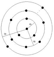
Figure 1: The figure depicts the general layered environment with one spin in the center of layers.

$$\Xi_{-}=\sum_{\mu=1}^{n}\alpha_{\mu}J^{\mu}_{-}.$$ (2.3)

Here, $\alpha$ coefficients specify interaction between system and environment and is dependent from distance. Also we have

$$J^{\mu}_{\pm}\equiv\sum_{j=1}^{N_{\mu}}\sigma^{j}_{\pm},$$ (2.4)

here, $\mu=1,2,\ldots,n$ for n different layers of bath. Also, we have

$$\sigma^{j}_{\pm}\equiv\frac{1}{2}(\sigma^{j}_{1}\pm i\sigma^{j}_{2}),$$

that represents the raising and lowering operators of the jth bath spin. The Heisenberg XX coupling has been found to be an effective Hamiltonian for the interaction of some quantum dot systems [18]. Equation(1) describes a very simple time independent interaction with equal coupling strength $\alpha_{1}$ for $N_{1}$ of first bath spin and $\alpha_{2}$ for $N_{2}$ of second bath spin to $\alpha_{n}$ for $N_{n}$ of nth bath spin. It is invariant under rotation around the $\textit{z}-axis$. The operator $J\equiv\frac{1}{2}\sum_{\mu=1}^{N}\sigma^{\mu}$ represents the total spin angular momentum of the bath (units are chosen such that $\hbar=1$). Therefore the central spin thus couples to the collective bath angular momentum.

We introduce an Orthonormal basis in the bath Hilbert space $H_{B}$ consisting of states $|j_{\mu},m_{\mu},x\rangle$ where $\mu$ is 1 to n. These states are defined as eigenstates of $\textbf{J}_{3}$ (eigenvalue m) and of $\textbf{J}^{2}$ (eigenvalue j(j+1)). The index $x$ labels the different eigenstates in the eigenspace $\textbf{{{K}}}_{j,m}$ belonging to a given pair (j,m) of quantum numbers. As usual, $j_{\mu}\leq\frac{N_{\mu}}{2}$ and $-j_{\mu}\leq m\leq j_{\mu}$ where $\mu$ is 1 to n. The dimension of $\textbf{{K}}_{j,m}$ is given by the expression [19, 20]

$$\Upsilon(j_{\mu},N_{\mu})=\left(\begin{array}[]{c}N_{\mu}\\ \frac{N_{\mu}}{2}-j_{\mu}\end{array}\right)-\left(\begin{array}[]{c}N_{\mu}\\ \frac{N_{\mu}}{2}-j_{\mu}-1\end{array}\right).$$ (2.5)

We assume that the initial state of the composite system be a product state. That is

$$\rho(0)=\rho_{S}(0)\otimes\rho_{B}(0).$$ (2.6)

We can calculate the reduced density matrix of the quantum system in the following expression.

$$\rho_{S}(t)=tr_{B}(U\rho(0)U^{{\dagger}}).$$ (2.7)

The above equation is obtained by doing partial-trace on bath and also U is the unitary operator which is defined as follows

$$U=\exp(-iHt).$$

The reduced density matrix is completely determined in terms of the Bloch vector

$$\chi(t)=\left(\begin{array}[]{c}\omega_{1}(t)\\ \omega_{2}(t)\\ \omega_{3}(t)\\ \end{array}\right)\equiv Tr(\sigma\rho_{S}(t)),$$ (2.8)

through the relationship

$$\rho_{S}(t)=\frac{1}{2}\left(\begin{array}[]{cc}1+\omega_{3}(t)&\omega_{1}(t)-i\omega_{2}(t)\\ \omega_{1}(t)-i\omega_{2}(t)&1-\omega_{3}(t)\\ \end{array}\right),$$ (2.9)

We note that the length $q(t)\equiv|\chi(t)|$ of the Bloch vector is equal to 1 iff $\rho_{S}(t)$ describes a pure state, and the von Neumann entropy S of the central spin can be expressed as a function of the length q(t) of the Bloch vector:

$$\emph{S}\equiv Tr[-\rho_{S}\ln\rho_{S}]=\ln 2-\frac{1}{2}(1-q)+\frac{1}{2}(1+q)\ln(1+q).$$ (2.10)

The initial state of the reduced system at t=0 is taken to be an arbitrary (possibly mixed) state

$$\rho_{S}(0)=\left(\begin{array}[]{cc}\frac{1+\omega_{3}(0)}{2}&\omega_{-}(0)\\ \omega_{+}(0)&\frac{1-\omega_{3}(0)}{2}\\ \end{array}\right),$$ (2.11)

while the spin bath is assumed to be in an unpolarized infinite temperature state:

$$\rho_{B}(0)=2^{-N}I_{B}.$$ (2.12)

Here, $I_{B}$ denotes the unit matrix in $H_{B}$ and N is $N_{1}+N_{2}+\ldots+N_{n}$, and we have defined the $\omega_{\pm}$ as linear combinations of the components $\omega_{1,2}$ of the Bloch vector

$$\omega_{\pm}=\frac{\omega_{1}\pm i\omega_{2}}{2}.$$ (2.13)

2.2 Reduced System Dynamics

In this section, we will derive the exact dynamics of the reduced density matrix $\rho_{S}(t)$ for our given model. We obtain the evolution of central spin with n different coupling coefficients that should be used from Eq.(7) until the solution model is exact. This yeilds

$$\rho_{S}(t)=tr_{B}\{i^{l}\sum_{l=0}^{\infty}\sum_{n=0}^{l}\frac{t^{l}}{l!}(-1)^{n}\left(\begin{array}[]{c}l\\ n\\ \end{array}\right)H^{n}(\rho_{S}(0)\otimes\frac{I_{B}}{2^{N}})H^{l-n}\}.$$ (2.14)

It can easily be verified that

$$H^{2k}=4^{k}[\sigma_{+}\sigma_{-}(\Xi_{-}\Xi_{+})^{k}+\sigma_{-}\sigma_{+}(\Xi_{+}\Xi_{-})^{k}],$$ (2.15)

and

$$H^{2k+1}=2\cdot 4^{k}[\sigma_{+}\Xi_{-}+\sigma_{-}\Xi_{+}].$$ (2.16)

We note that such simple expressions are obtained since a term $\sigma_{3}J_{3}$ is missing in the interaction Hamiltonian. We substitute the last two equations into Lindblad equation[10] as follows

$$L^{l}\rho=i^{l}\sum_{n=0}^{l}(-1)^{n}\left(\begin{array}[]{c}l\\ n\\ \end{array}\right)H^{n}\rho H^{l-n},$$ (2.17)

to get the formulas

$$tr_{B}\{\ L^{2l+1}\rho_{S}(0)\otimes\ 2^{-N}I_{B}\}=0,$$ (2.18)

and

$$tr_{B}\{\ L^{2l}\rho_{S}(0)\otimes\ 2^{-N}I_{B}\}=\sum_{l=0}^{\infty}(-4)^{l}\sum_{n=0}^{2l}\frac{t^{2l}}{(2l)!}\left(\begin{array}[]{c}2l\\ 2n\\ \end{array}\right)[(\frac{1+\omega_{3}\sigma_{3}}{2})\Omega_{l}+(\omega_{+}\sigma_{-}+\omega_{-}\sigma_{+})\Gamma^{l-n}_{n}],$$ (2.19)

which hold for all l=1,2,…. Here,we have introduced the bath correlation functions

$$\Omega_{l}\equiv\frac{1}{2^{N}}tr_{B}\{(\Xi_{+}\Xi_{-})^{l}\},$$ (2.20)

$$\Gamma^{l-n}_{n}\equiv\frac{1}{2^{N}}tr_{B}\{(\Xi_{+}\Xi_{-})^{l-n}(\Xi_{-}\Xi_{+})^{n}\},$$ (2.21)

where we have product $\Xi_{\pm}\Xi_{\mp}$ as follows

$$\Xi_{\pm}\Xi_{\mp}=(\sum_{\mu=1}^{n}\alpha_{\mu}J^{\mu}_{\pm})(\sum_{\mu=1}^{n}\alpha_{\mu}J^{\mu}_{\mp}).$$ (2.22)

Of course, Eq.(18) is zero because it is

$$\langle j,m|J_{\pm}|j,m\rangle=0.$$

We will come back to these correlation functions when we discuss approximation techniques in Sec.(4).

Using the formulas (18) and (19) in Eq.(14) we can express the components of the Bloch vector as follows,

$$\omega_{\pm}(t)=f_{\pm}(t)\omega_{\pm}(0),$$ (2.23)

$$\omega_{3}(t)=f_{z}(t)\omega_{3}(0),$$ (2.24)

where we have introduced the functions

$$f_{\pm}(t)\equiv tr_{B}\{\cos[2th_{1}(\alpha_{1},\ldots,\alpha_{n})]\cos[2th_{2}(\alpha_{1},\ldots,\alpha_{n})]\otimes 2^{-N}I_{B}\},$$ (2.25)

and

$$f_{z}(t)\equiv tr_{B}\{\cos[2th_{1}(\alpha_{1},\ldots,\alpha_{n})]\otimes 2^{-N}I_{B}\},$$ (2.26)

where $h_{1}(\alpha_{1},\alpha_{2},\ldots,\alpha_{n})$ and $h_{2}(\alpha_{1},\alpha_{2},\ldots,\alpha_{n})$ are

$$h_{1}(\alpha_{1},\alpha_{2},\ldots,\alpha_{n})=\sqrt{\sum_{\mu=1}^{n}\alpha^{2}_{\mu}J^{\mu}_{+}J^{\mu}_{-}},$$ (2.27)

$$h_{2}(\alpha_{1},\alpha_{2},\ldots,\alpha_{n})=\sqrt{\sum_{\mu}^{n}\alpha^{2}_{\mu}J^{\mu}_{-}J^{\mu}_{+}}.$$ (2.28)

Calculating the traces over the spin bath in the eigenbasis of $J_{3}$ and $\textbf{J}^{2}$ using

$$J_{\pm}J_{\mp}|j,m,x\rangle=(j\pm m)(j\mp m+1)|j,m,x\rangle.$$ (2.29)

We find

$$f_{\pm}(t)=[\prod_{i=1}^{n}\sum_{j_{i},m_{i}}\Upsilon(N_{i},j_{i})]\frac{\cos(4t\sqrt{\zeta})\cos(4t\sqrt{\eta})}{2^{\sum_{i=1}^{n}}N_{i}},$$ (2.30)

and

$$f_{z}(t)=[\prod_{i=1}^{n}\sum_{j_{i},m_{i}}\Upsilon(N_{i},j_{i})]\frac{\cos(4t\sqrt{\zeta})}{2^{\sum_{i=1}^{n}}N_{i}},$$ (2.31)

here,$\zeta$ and $\eta$ denoted are as

$$\zeta=\sum_{i=1}^{n}h_{i}^{+}\alpha_{i}^{2},$$

and

$$\eta=\sum_{i=1}^{n}h_{i}^{-}\alpha_{i}^{2},$$

and also, we have

$$h_{i}^{+}=h(j_{i},m_{i});h_{i}^{-}=h(j_{i},-m_{i}),$$

where we have introduced the quantity $h(j,\pm m)=(j\pm m)(j\mp m+1)$.

Thus we have determined the exact dynamics of the reduced system: The density matrix $\rho_{S}(t)$ of the central spin is given through the components of the Bloch vector which are provided by the relations (23),(24) and (30),(31). We note that the dynamics can be expressed completely through only two real-valued function $f_{\pm}(t)$ and $f_{z}(t)$. This fact is connected to the rotational symmetry of the system. Also from the overall role of coupling coefficients and degeneracy coefficients in the relations (30) and (31), it will be shown that the study of control over decoherence is on coupling coefficients and degeneracy coefficients that you’ll see Sec.(3).

3 Example

In this example, we consider the central spin with two different bath by two different coupling coefficients. This means we consider two layers with different radii. The choice of different coupling coefficients certainly will affect on degeneracy coefficient because the behavior of particles in each layer is different from other layers and this difference is to express the considering by different coupling coefficients and different degeneracy coefficients. So,we consider our hamiltonian as

$$H=2(\sigma_{+}\Xi_{-}+\sigma_{-}\Xi_{+}),$$ (3.32)

where we define $\Xi$ as

$$\Xi_{+}=\sum_{\mu=1}^{2}\alpha_{\mu}J^{\mu}_{+},$$

$$\Xi_{-}=\sum_{\mu=1}^{2}\alpha_{\mu}J^{\mu}_{-}.$$

According to the introduced model, we can express two real-valued functions $f_{\pm}(t)$ and $f_{z}(t)$ as

$$f_{\pm}(t)=\sum_{j_{1},m_{1}}\sum_{j_{2},m_{2}}\Upsilon(N_{1},j_{1})\Upsilon(N_{2},j_{2})\frac{\cos(2t\sqrt{\beta})\cos(2t\sqrt{\gamma})}{2^{N_{1}+N_{2}}},$$ (3.33)

and

$$f_{z}(t)=\sum_{j_{1},m_{1}}\sum_{j_{2},m_{2}}\Upsilon(N_{1},j_{1})\Upsilon(N_{2},j_{2})\frac{\cos(4t\sqrt{\beta})}{2^{N_{1}+N_{2}}},$$ (3.34)

where $\beta$ and $\gamma$ are denoted as

$$\beta=\alpha^{2}_{1}h(j_{1},m_{1})+\alpha^{2}_{2}h(j_{2},m_{2}),$$

and

$$\gamma=\alpha^{2}_{1}h(j_{1},-m_{1})+\alpha^{2}_{2}h(j_{2},-m_{2}).$$

The explicit solution constructed in the previous section takes on a relatively simple form in the limit $N\rightarrow\infty$ of an infinite number of bath spins [10]. Because N is $N_{1}+N_{2}$, we should discuss about $N_{1}\rightarrow\infty$ or $N_{2}\rightarrow\infty$ or both. in Ref.[10] for large $N$, the corresponding correlation function is obtained. But here by considering two layers, we obtain the states of $N_{1}\rightarrow\infty$ and $N_{2}\rightarrow\infty$ for corresponding correlation functions as follows:

$$\Omega_{l}\approx\sum_{k=0}^{l}\left(\begin{array}[]{c}l\\ k\\ \end{array}\right)(l-k)!k!\frac{\alpha_{1}^{2(l-k)}\alpha_{2}^{2k}}{2^{l}},$$ (3.35)

$$\Gamma_{n}^{l-n}\approx\sum_{k=0}^{n}\sum_{\acute{k}=0}^{l-n}\left(\begin{array}[]{c}n\\ k\\ \end{array}\right)\left(\begin{array}[]{c}l-n\\ \acute{k}\\ \end{array}\right)\frac{(n-k)!(l-n-\acute{k})!k!\acute{k}!\alpha_{1}^{2(n-k)}\alpha_{2}^{l-n-\acute{k}}}{2^{l}}.$$ (3.36)

Of course, we assume a non-trivial finite limit $N_{i}\rightarrow\infty$, therefore we rescale the coupling constant as[10],

$$\alpha_{i}\rightarrow\frac{\alpha_{i}}{\sqrt{N_{i}}}.$$ (3.37)

Using this approximation in Eq.(19), we can rewrite $f_{\pm}$ and $f_{z}$ as

$$f_{\pm}(t)=\sum_{l=0}^{\infty}\sum_{n=0}^{2l}\sum_{k=0}^{n}\sum_{\acute{k}=0}^{l-n}\frac{(-2)^{l}t^{2l}}{(2l)!}\left(\begin{array}[]{c}2l\\ 2n\\ \end{array}\right)\left(\begin{array}[]{c}n\\ k\\ \end{array}\right)\left(\begin{array}[]{c}l-n\\ \acute{k}\\ \end{array}\right)k!\acute{k}!(n-k)!(l-n-\acute{k})!\alpha_{1}^{2(l-n-\acute{k})}\alpha_{2}^{2(n-k)},$$ (3.38)

and

$$f_{z}(t)=\sum_{l=0}^{\infty}\sum_{k=0}^{l}\frac{(-8)^{l}t^{2l}}{(2l)!}\left(\begin{array}[]{c}2l\\ 2n\\ \end{array}\right)(l-k)!k!\alpha_{1}^{2(l-k)}\alpha_{2}^{2k}.$$ (3.39)

The up state is a state with consideration to $N_{1}\rightarrow\infty$ and $N_{2}\rightarrow\infty$, which is for the most general level cases non-trivial for an infinite limit. But there might be a layer which has a finite number of particle and another one with an infinite number of particle (of course here, it is understandable that infinite means the order of Avogadro’s number because this size of particles in the scale of our study, accounts for infinity). We assume that $N_{2}$ is limited and $N_{1}$ is unlimited. Of course in computing because of the symmetry of the system, there isn’t any difference is taking $N_{1}$ limited and $N_{2}$ unlimited with the previous case. So, for $N_{1}\rightarrow\infty$ we can obtain as

$$f_{\pm}(t)=\frac{1}{2^{N_{2}}}\sum_{j_{2},m_{2}}\sum_{n=0}^{\infty}\sum_{k=0}^{\infty}\Upsilon(N_{2},j_{2})\cos(2t\alpha_{2}\sqrt{h(j_{2},m_{2})})\cos(2t\alpha_{2}\sqrt{h(j_{2},-m_{2})})$$

$$\times\frac{(-2)^{n}t^{2n}}{(2n)!}n!\frac{(-2)^{k}t^{2k}}{(2k)!}k!\alpha_{1}^{2(n+k)},$$ (3.40)

and

$$f_{z}(t)=\frac{1}{2^{N_{2}}}\sum_{j_{2},m_{2}}\Upsilon(N_{2},j_{2})\cos(4t\alpha_{2}\sqrt{h(j_{2},m_{2})})\{1-2\sqrt{2}t\alpha_{1}DF[\sqrt{2}t\alpha_{1}]\}.$$ (3.41)

Note that Dawson Function is closely related to the error function erf, as

$$DF(x)=\frac{\sqrt{\pi}}{2}\exp(-x^{2})erfi(x),$$

where erfi is the imaginary error function, $erfi(x)=-ierf(ix)$.

4 approximation techniques

In this section we will apply different approximation techniques to the spin star model introduced and discussed in the previous section. Due to the simplicity of this model we can not only integrate exactly the reduced system dynamics, but also construct explicitly the various master equations for the density matrix of the central spin and analyze and compare their perturbation expansions. In the following discussion we will stick to the Bloch vector notation. Each of the master equations obtained can easily be transformed into an equation involving Lindblad superoperators using the translations rules

$$\rho_{S}=\frac{I+\omega_{3}\sigma_{3}}{2}+\omega_{+}\sigma_{-}+\omega_{-}\sigma_{+}.$$ (4.42)

The second order approximation of the master equation for the reduced system is usually obtained within the Born approximation [5]. It is equivalent to the second order of the Nakajima-Zwanzing projection operator technique. In our model the Born approximation leads to the master equation

$$\dot{\rho}_{S}(t)=-\int_{0}^{t}dstr_{B}\{[H,[H,\rho_{S}(s)\otimes\rho_{B}(0)]]\}=-8\Omega_{1}\int_{0}^{t}ds(\omega(s)_{3}\sigma_{3}+\omega(s)_{+}\sigma_{-}+\omega(s)_{-}\sigma_{+}),$$ (4.43)

where the bath correlation function is found to be

$$\Omega_{1}=\frac{1}{2^{N}}tr_{B}\{\Xi_{+}\Xi_{-}\}=\frac{1}{2^{N}}tr_{B}\{(\alpha_{1}J^{1}_{+}+\alpha_{2}J^{2}_{+})(\alpha_{1}J^{1}_{-}+\alpha_{2}J^{2}_{-})\}=\frac{1}{2}(\alpha_{1}^{2}N_{1}+\alpha_{2}^{2}N_{2}).$$ (4.44)

It is important to notice that $\Omega_{1}$, as well as all other bath correlation functions are independent of time. This is to be contrasted to those situations in which the bath correlation function decay rapidly and which allow the derivation of a Markovian master equation. The time-independence of the correlation function is the main reason for the non-Markovian behavior of the spin bath model. The integro-differential Eq.(43) can easily be solved by a Laplace transformation with the solution

$$f_{\pm}(t)=\frac{\omega_{\pm}(t)}{\omega_{\pm}(0)}=\cos(2t\sqrt{\delta}),$$ (4.45)

$$f_{z}(t)=\frac{\omega_{3}(t)}{\omega_{3}(0)}\cos(2t\sqrt{2\delta}),$$ (4.46)

where $\delta$ is denoted as

$$\delta=\alpha_{1}^{2}N_{1}+\alpha_{2}^{2}N_{2}.$$ (4.47)

In many physical applications the integration of the integro-differential equation is much more complicated and one tries to approximate the dynamics through a master equation which is local in time. To this end, the terms $\omega_{\pm}(t)$ and $\omega_{3}(t)$ under the integral in Eq.(43) are replaced by $\omega_{\pm}(t)$ and $\omega_{3}(t)$, respectively. We thus arrive at the time-local master equation

$$\frac{d}{dt}\rho_{s}(t)=-4\delta\int_{0}^{t}ds(\omega_{3}(t)\sigma_{3}+\omega_{+}(t)\sigma_{-}+\omega_{-}(t)\sigma_{+})=-4\delta t(\omega_{3}(t)\sigma_{3}+\omega_{+}(t)\sigma_{-}+\omega_{-}(t)\sigma_{+}),$$ (4.48)

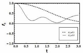
Figure 2: The equal spin numbers for correlation function $f_{\pm}$ [see Eqs.(33)], with $\alpha=0.1$ and $N_{i}=20$.

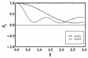
Figure 3: The changes of spin number of layers for correlation function $f_{\pm}$ [see Eqs.(33)], with $\alpha=0.1$, $N_{1}=20$ and $N_{2}=100$.

which is sometimes referred to as Redfield equation. Also this master equation is easily solved to give the expressions

$$f_{\pm}(t)=\exp(-2\delta t),$$ (4.49)

$$f_{z}(t)=\exp(-4\delta t).$$ (4.50)

The Redfield equation is equivalent to the second order of the time-convolutionless projection operator technique. finally, In order to obtain, a Markovian master equation, i.e. a time-local

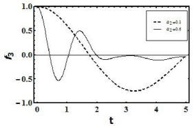
Figure 4: The equal spin numbers for correlation function $f_{3}$ [see Eqs.(34)],with $\alpha=0.1$ and $N_{i}=20$ .

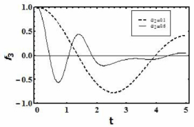
Figure 5: The changes of spin number of layers for correlation function $f_{3}$ [see Eqs.(34)], with $\alpha=0.1$, $N_{1}=20$ and $N_{2}=100$.

equation involving a time independent generator, one pushes the upper limit of the integral in Eq.(48) to infinity, as other studies of the master equation. This limit leads to the Born-Markov approximation of the reduced dynamics. In the present model, however, it is not possible to perform this approximation because the integrand does not vanish for large t. Thus,the Born-Markov limit does not exist for the spin bath model investigated here and the description of decoherence processes requires the usage of non-Markovian methods.

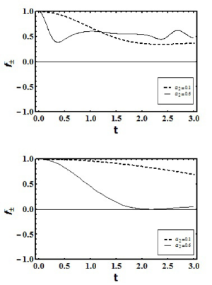
Figure 6: Comparison of limit $N\rightarrow\infty$ with limit $N_{1}\rightarrow\infty$ or $N_{2}\rightarrow\infty$ for the changes of correlation function $f_{\pm}$ [see Eqs.(38) and Eqs.(40)], with $\alpha=0.1$ and $n=20$.

5 conclusion

With the help of a simple analytically solvable model of a spin star system, we have considered layered environment model with one-qubit in centr of layers and every layer is constructed by some spins. Of course, we have assumed these layers have different radii which means different coupling coefficients. By considering the Fig.(2) and Fig.(4), and selecting equal degeneracy coefficients of both layers and considering the influence of coupling coefficients in decoherence-time control it can be deduced that the fluctuations in $f_{z}$ is more intense than $f_{\pm}$. Meanwhile variations of coupling coefficients, makes the fluctuations

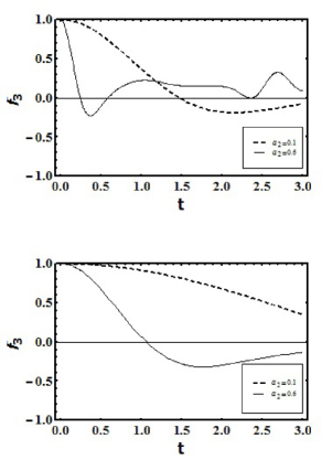
Figure 7: Comparison of limit $N\rightarrow\infty$ with limit $N_{1}\rightarrow\infty$ or $N_{2}\rightarrow\infty$ for the changes of correlation function $f_{3}$ [see Eqs.(39) and Eqs.(41)], with $\alpha=0.1$ and $n=20$.

of $f_{z}$ greater than $f_{\pm}$. In Fig.(4) one can see that the increase of fluctuations can allow us to control, the decoherence. but it’s not good at $f_{\pm}$ because near zero, fluctuations are gentle (this means that the amplitude of oscillation is shorter and the course is slowly changing). Previous time of the system (at short period of times) is longer than the decoherence time at $f_{z}$ and is pulsed and is shorter at $f_{\pm}$ and continuous. As a result, in general case for $f_{z}$ and $f_{\pm}$ to increasing the power of coupling coefficient, yields greater control on decoherence and increase of decoherence time. Also, with by considering Fig.(3) and Fig.(5) and selecting inequal degeneracy coefficients, we find that the same effects of selecting equal degeneracy coefficients in Fig.(2) and Fig.(4) take place, but in this part, fluctuations are more and the carve shifts towards the vertical axis. It should again be emphasized that at $f_{z}$ transformation from coherence mode to decoherence mode and vice versa is pulsed and at $f_{\pm}$ the decoherence is controlled continuously. Then, we have considered the limit $N\rightarrow\infty$ and for a special example (two layers with different couple coefficients) showed that $N_{1}\rightarrow\infty$ with $N_{2}\rightarrow\infty$ have equal result. By considering Fig.(6), the first chart is related to when $N_{1}\rightarrow\infty$ and $N_{2}\rightarrow\infty$, and the second chart is when $N_{1}\rightarrow\infty$ or $N_{2}\rightarrow\infty$. In the first case we can find that the fluctuations are increased by the increase of coupling strength, this can also be seen in the second case too. But the difference between first and second situation is in decoherence-time control that in the first situation, this work is well done because the curve in the first graph is distant from the limit of zero and this means the increase in decoherence-time control. Thus the best case is when $N_{1}\rightarrow\infty$ and $N_{2}\rightarrow\infty$ occur simultaneously, which is more general and real. It is much better because decoherence time is controled better. In Fig.(7) we have the same conclusion. In Fig.(6) and Fig.(7) we can see that we have more intensity in fluctuations of $f_{z}$ than $f_{\pm}$, be side decoherence time at $f_{\pm}$ is better than $f_{z}$ because at $f_{3}$ transformation of states from coherence mode to decoherence mode and vice versa is pulsed.

References

• [1] M.A.Nielsen and I.L.Chuang, Quantum Computation and Quantum Information (Cambridge University Press, Cambridge, 2000).
• [2] D.Loss and D.P.DiVincenzo, Quantum computation with quantum dots , Phys. Rev. A57, 120 (1998).
• [3] B.E.Kane, A silicon-based nuclear spin quantum computer , Nature 393, 133 (1998).
• [4] D.D.Awschalom, N.Samarth, and D.Loss, Semiconductor Spintronics and Quantum Computation (Springer, New York, 2002).
• [5] H.P.Beruer, F.Petruccione, The Theory Of Open Quantum System (Oxford University Press, Oxford, 2002).
• [6] E.C.G.Sudarshan, P.M.Mathews and J.Rau, Stochastic dynamics of quantum-mechanical systems , Phys. Rev. 121, 920 (1961).
• [7] A.Hutton, S.Bose, Mediated entanglement and correlations in a star network of interacting spins , Phys. Rev. A 69 042312 (2004).
• [8] Y.Hamdouni, M.Fannes and F.Petruccione, Exact dynamics of a two-qubit system in a spin star environment, Phys. Rev. B 73, 245323 (2006).
• [9] Y.Hamdouni, An exactly solvable model for the dynamics of two spin-$\frac{1}{2}$ particles embedded in separate spin star environments, J. Phys. A: Math. Theor. 42 315301 (2009).
• [10] H.P.Breuer, D.Burgerth, F.Petruccione, Non-Markovian dynamics in a spin star system: Exact solution and approximation techniques , Phys. Rev. B 70 045323 (2004).
• [11] V.Semin, I.Sinayskiy and F.Petruccione, Initial correlation in a system of a spin coupled to a spin bath through an intermediate spin , Phys. Rev. A. 86, 062114 (2012).
• [12] H.Krovi, O.Oreshkov, M.Ryazanov, D.A.Lidar, Non-Markovian dynamics of a qubit coupled to an Ising spin bath , Phys. Rev. A 76(5), 052117 (2007).
• [13] E.Ferraro, H.P.Breuer, A.Napoli, M.A.Jivulescu, A.Messina, Non-Markovian dynamics of a single electron spin coupled to a nuclear spin bath , Phys. Rev. B 78(6), 064309 (2008).
• [14] D.Rossini, P.Facchi, R.Fazio, G.Florio, D.A.Lidar, S.Pascazio, F.Plastina, P.Zanardi, Bang-Bang control of a qubit coupled to a quantum critical spin bath , Phys. Rev. A 77(5), 052112 (2008)
• [15] C.M.Dawson, H.P.Hines, R.H.Mckenzie, G.J.Milbrun, Entanglement sharing and decoherence in the spin-bath , Phys. Rev. A 71 052321 (2005).
• [16] W.H.Zurek. Decoherence and the transition from quantum to classical REVISITED. arXiv:quant-ph/0306072, June 2003.
• [17] E.H.Lieb, T.D.Shultz, D.C.Mattis, Ann. Phys. (N.Y.) 16 407 (1961) also reprinted in The Many-Body Problem by D. C. Mattis (World Scientific, Singapore, 1993).
• [18] A.Imamoglu, D.D.Awschalom, G.Burkard, D.P.Divincenzo, D.Loss, M.Sherwin, A.Small, Quantum Information Processing Using Quantum Dot Spins and Cavity QED , Phys. Rev. Lett. 83 4204 (1999).
• [19] A.Hutton, S.Bose, Mediated Entanglement And Correlations In A Star Network Of Interacting Spins , quant-ph/ 0208114 (2002).
• [20] J.Wesenberg, K.MΓΈlmer, Mixed collective states of many spins , Phys. Rev. A 65 062304 (2002).