Front speed in reactive compressible stirred media

Abstract

We investigated a nonlinear advection-diffusion-reaction equation for a passive scalar field. The purpose is to understand how the compressibility can affect the front dynamics and the bulk burning rate. We study two classes of flows: periodic shear flow and cellular flow both in the case of fast advection regime, analysing the system at varying the extent of compressibility and the reaction rate. We find that the bulk burning rate $v_{f}$ in a shear flow increases with compressibility intensity, $\epsilon$, following a relation $\Delta v_{f}\sim\epsilon^{2}$. Furthermore, the faster the reaction the more important the difference with respect to the laminar case. The effect has been quantitatively measured and it turns out to be generally little. For the cellular flow, the two extreme cases have been investigated, with the whole perturbation situated either in the centre of the vortex or in the periphery. The dependence in this case does not show a monotonic scaling with different behaviour in the two cases. The enhancing remains modest and always less than $20\%$.

I Introduction

The dynamics of reacting species presents several issues of great interest from a theoretical point of view xin ; Constantin:2000p15663 ; Ver_12 . Moreover it is also a problem of wide application in many fields, from front propagation in gases combustion , chemical reaction in liquids chem ; e95 and ecological dynamics of biological systems (e.g. plankton in oceans) bio ; alplmb00 ; guasto2012fluid ; korolev2010genetic ; d2010fluid .

In the most simplest model of reaction dynamics, the state of the system is described by a single scalar field $\theta({\bf r},t)$, that represents the concentration of products. The field $\theta$ vanishes in the regions filled with fresh material (the unstable phase), equals unity where only inert products are left (the stable phase) and takes intermediate values wherever reactants and products coexist, i.e., in the region where production takes place. In their seminal contributions, Fisher, Kolmogorov, Petrovskii and Piskunov FKPP ; f37 (FKPP) considered the simplest case of pure reaction/diffusion and proposed the so-called FKPP model

$$\partial_{t}\theta=D\Delta\theta+f(\theta)\,,$$ (I.1)

where $D$ is the molecular diffusivity and $f(\theta)$ describes the reaction process that obviously depends on the phenomenon under investigation. In this work, as in the original works of FKPP, we focus on pulled reaction, e.g. the autocatalytic reaction $f=\alpha\theta(1-\theta)$, where $\alpha$ is the reaction rate and its inverse, $\tau=1/\alpha$, is the reaction time.

However, most natural phenomena take place in deformable media like fluids and therefore transport properties cannot be ignored. If the medium is stirred, e.g. an eulerian velocity field $\mathbf{u}(\mathbf{x})$ is present, Eq. (I.1) can be generalized in the incompressible case to

$$\partial_{t}\theta+(\mathbf{u}\cdot\mathbf{\nabla})\theta=D\Delta\theta+f(\theta)\,\,.$$ (I.2)

The complete mathematical description of these phenomena is given by partial differential equations (PDE) for the coupled evolution of the velocity field and of the concentration of the reacting species combustion . Therefore the above Eq. (I.2) should be coupled with Navier-Stokes equations (usually in a non trivial way). This is the general framework for treating engineering combustion problems in gases Peters ; prudhomme ; poinsot . In some cases, e.g. vladimirova2003model , the coupling can be simplified using a Boussinesq term.
In this work, as a further simplification, we assume that the reactants do not influence the velocity field which evolves independently. In such a limit the dynamics is still non trivial and it is completely described by the above ARD Eq. (I.2) together with the proper definition of a given velocity field, $\mathbf{u}(\mathbf{x})$. This equation has been intensively studied in incompressible media audoly ; vladimirova2003flame ; acvv1 ; ctvv . In particular, it has been investigated the dependence of the front speed as a function of $D,\alpha$ and the velocity field $\mathbf{u}(\mathbf{x})$ acvv .

On the contrary, in the case of compressible flows, the ARD problem did not receive too much attention but only recently in a mathematical framework constantin2008propagation ; benzi . To account for compressible flows is indeed not simple but it is a relevant issue in combustion Peters ; poinsot , plankton dynamics in turbulent flows lewis2000planktonic and also in particle-laden flows, where the particle phase can be highly compressible even in incompressible flows, because of inertia Min_01 ; falkovich2001particles ; bec_07 . While the passive scalar approximation for reactive species is hardly tenable in gas combustion phenomena, it may be considered appropriate in aqueous or liquid reactions (notably plankton in oceans) and for dilute particle-laden flows. In those cases, it may give some relevant insights for front propagation and can be used as a model for the flame tracking in some limitsvladimirova2006flame .

Our aim is to investigate the effects of the compressibility to the bulk burning rate of the reaction process by studying the following PDE:

$$\rho\left[\frac{\partial\theta}{\partial t}+u_{i}\frac{\partial\theta}{\partial x_{i}}\right]=D_{0}\frac{\partial^{2}\theta}{\partial x_{i}^{2}}+f(\theta)$$ (I.3)

The scalar field $\theta$ represents the mass fraction of a single species of a binary mixture, while $u_{i}$ is the $i^{th}$ component of a given compressible flow, $D_{0}=\rho D$ is the diffusion coefficient (supposed to be constant), $f(\theta)=\dot{\omega}$ the rate of production of the chosen species and $\rho$ the non constant density of the fluid.

The paper is organized as follows: Section II is devoted to the presentation of the model and the principal aspects of the numerical computations. In Section III we discuss the results for the front propagation in compressible shear flows. Section IV is devoted to the case of compressible cellular flows. Finally, in Section V, the reader can find the conclusions.

II The model

The PDE model described by Eq. (I.3) can be derived from the equation of conservation of species, that is relevant for combustion dynamics combustion ; prudhomme . Let us consider two species (namely A,B) which diffuse and react together while they are passively transported by a compressible flow, being $\rho_{A}(x,y,t)$ the mass of species $A$ per unit volume, the conservation of species $A$ gives:

$$\frac{\partial{\rho_{A}}}{\partial t}+\frac{\partial}{\partial x_{i}}\left[{\rho_{A}(u_{i}+U_{A,i})}\right]=\dot{\omega}_{A}$$ (II.1)

where $u_{i}$ is the $i^{th}$ component of the advective flow field, $U_{A,i}$ is the velocity of diffusion of species $A$ and $\dot{\omega}_{A}$ is the rate of production.

Define the mass fraction $Y_{k}=\rho_{k}/\rho$, where $\rho$ is the density of the mixture and $k=A,B$. The species conservation can be written in terms of mass fraction as follows:

$$\frac{\partial{(\rho Y_{k})}}{\partial t}+\frac{\partial}{\partial x_{i}}\left[{\rho Y_{k}(u_{i}+U_{k,i})}\right]=\dot{\omega}_{k}$$ (II.2)

Where $Y_{A}+Y_{B}=1$. Moreover, if Fick’s law is considered, the diffusion velocities can be defined as follow:

$$Y_{A}U_{A,i}=-Y_{B}U_{B,i}=-D\frac{\partial Y_{A}}{\partial x_{i}}$$ (II.3)

In the following, we assume an auto-catalytic irreversible law $A+B\xrightarrow{}2A$:

$$\dot{\omega}_{A}=\alpha{\rho_{A}\rho_{B}}=\alpha\rho^{2}Y_{A}Y_{B}=\alpha\rho^{2}Y_{A}(1-Y_{A})$$ (II.4)

where the constant $\alpha$ controls the speed of reaction and by definition $\dot{\omega}_{A}=-\dot{\omega}_{B}.$

Thus, the evolution of the mass fraction of species A is completely described by the following PDE:

$$\rho\left[\frac{\partial\theta}{\partial t}+u_{i}\frac{\partial\theta}{\partial x_{i}}\right]=D_{0}\frac{\partial^{2}\theta}{\partial x_{i}^{2}}+\alpha\rho^{2}\theta(1-\theta)\,,$$ (II.5)

that holds if we neglect the coupling between conservation of species equation and the conservation of energy equation. That is the case in which the energy released by the reaction is negligible and thus the momentum and energy equations evolve independently. The left hand side of Eq. (II.5) is written in non-conservative form using the continuity equation of the mixture and the product $\rho D=D_{0}$ is assumed constant (which is quite a reasonable hypothesis Peters ; prudhomme ).

Since we are interested, in the front propagation, we consider the following geometry:

$$-\infty<x<\infty\leavevmode\nobreak\ \leavevmode\nobreak\ ,\leavevmode\nobreak\ \leavevmode\nobreak\ 0\leq y\leq L$$ (II.6)

Only for the sake of simplicity we assume periodic boundary conditions in the $y-$direction and $\theta(-\infty,y,t)=1$ (burned material in a combustion terminology) and $\theta(\infty,y,t)=0$ (fresh material).

At $t=0$ the initial condition is given by:

$$\theta(x,y,t)=\left\{\begin{array}[]{ll}1&\textrm{if $x<0$}\\ 0&\textrm{if $x\geq 0$}\end{array}\right.$$ (II.7)

Of course different boundary and initial conditions may be interesting. For instance, if one is interested in quenching issues, appropriate initial conditions would pose $\theta$ initially localized in a region of size $\ell$

$$\theta(x,y,0) = \left\{\begin{array}[]{ll}1&\textrm{if $-\ell/2\leq x\leq\ell/2$}\\ 0&\textrm{if $x<-\ell/2$ or $x>\ell/2$}\end{array}\right.\,.$$ (II.10)

Equation (II.5) has been solved using a eighth-order central finite difference scheme in space and a fourth-order Runge-Kutta integration in time. The grid size is sufficiently small to guarantee a good representation of the shear across the reacting region and convergence of solutions has been verified. To compute accurately the asymptotic mean bulk burning rate, very long integration periods are required. The grid is remapped following the reacting front and the computational domain is extended upstream and downstream from the reactive zone so that the boundary effects are negligible.

III Compressible shear flow

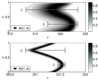
Figure 1: Shape of the active part of the front (we use the function $4\theta(1-\theta)$, which is maximal for $\theta=0.5$), for a fixed Peclet number ($Pe=100$) and for two different reaction rates. Taking as reference the incompressible test case ($\epsilon=0$) we can define two different thicknesses. The bare front thickness as $\delta\sim\sqrt{D/\alpha}$ and the distance between the tip and the tail of the reacting region $\Delta$. For a slow reaction (upper panel, $Da=1$), we have approximately $\Delta\approx 10$ and $\delta\approx 6$. For fast reaction (lower panel, $Da=100$) $\Delta\approx 0.8$ and $\delta\approx 0.15$.

We investigate the effects of compressibility in a 2D steady-state shear flow using the velocity field

$$\bar{u}(x,y)=\left(\frac{U_{0}\sin\left(\frac{2\pi y}{L}\right)}{1+\epsilon\sin\left(\frac{2\pi x}{\lambda}\right)},0\right)\,.$$ (III.1)

Such a choice corresponds to a Kolmogorov flow with amplitude $U_{0}$ and wavelength $L$, perturbed by a steady wave of wavelength $\lambda$ and magnitude $\epsilon$ accounting for the compressibility of the flow. Let us stress that the perturbation is oriented along the direction of propagation of the reactive front, i.e. the $x$ axis.
In order to satisfy the continuity equation, $\partial_{i}(\rho u_{i})=0$, it is necessary to impose a spatially dependence on $\rho$, as

$$\rho(x)=\rho_{0}\left[1+\epsilon\sin\left(\frac{2\pi x}{\lambda}\right)\right]\,.$$

Finally, Eq. (II.5) can be written in non-dimensional form:

$$\frac{\partial\theta}{\partial t^{*}}+u^{*}_{i}\frac{\partial\theta}{\partial x^{*}_{i}}=\frac{1}{\rho^{*}Pe}\frac{\partial^{2}\theta}{\partial{x^{*}_{i}}^{2}}+{\rho^{*}}Da\theta(1-\theta)$$ (III.2)

if we define $\rho^{*}=\rho/\rho_{0}$, $x_{i}^{*}=x_{i}/L$, $u_{i}^{*}=u_{i}/U_{0}$, $t^{*}=(tU_{0})/L$.
The adimensional parameters $Pe=(\rho_{0}U_{0}L)/D_{0}$ and $Da=(L\alpha\rho_{0})/U_{0}$ are the Peclet and the Damköhler numbers which define the ratio between the diffusive and advective time scale and the ratio between the advective and reactive time scale respectively.

In the following, we will drop the star notation and we will solve Eq. (III.2) focusing on regimes at high Peclet number $Pe\gg 1$. Varying the Damköhler number in a range of $Da\in[1,1000]$, we will quantify the effects of $\lambda$ and $\epsilon$ on the asymptotic value of the bulk burning rate.

The instantaneous bulk burning rate is:

$$v_{f}(t)=\int_{0}^{1}\int_{0}^{+\infty}\dot{\omega}\leavevmode\nobreak\ dxdy=\int_{0}^{1}\int_{0}^{+\infty}Da\rho^{2}\theta(1-\theta)\leavevmode\nobreak\ dxdy\,,$$ (III.3)

while the mean or asymptotic bulk burning rate is defined as the time average of $v_{f}(t)$ over a sufficiently long interval:

$$v=\frac{1}{T}\int_{0}^{T}v_{f}(t)dt$$ (III.4)

To shed some light on the role played by $\lambda$ we first run a simulation in absence of compressibility for two different Damköhler (slow and fast reaction) and for a fixed Peclet. We characterize the thicknesses of the reactive front $\Delta$ and $\delta$ (see Figure 1 for definition). From this figure, it is clear that the faster the reaction the thinner the flame.

Then we have carried out simulations in which the compressibility is fixed ($\epsilon=0.5$) and we choose $\lambda$ approximately greater, lower or between the two thicknesses computed in the case of zero compressibility.
In Figure 2 we show how the geometrical aspect of the reactive front changes by varying $\lambda$. In the low density zones, the front thickness appears broader than in high density zones due to the decreasing of the local Peclet and Damköhler number ($Pe_{l}=\rho Pe$, $Da_{l}=\rho Da$). Compressibility perturbation wrinkles the front in the small-wavelength limit, whereas for large wavelengths it is only corrugated, since the entire reactive-diffusive front is embedded in a wavelength. Nevertheless, even though the front does not appear stationary (even in a co-moving reference system) and it is noticeably distorted by the presence of compressibility, the mean velocity of propagation ($v$) does not change, see Figure 3. The wavelength of the perturbation controls the frequency and the magnitude of the instantaneous value of the front speed but does not affect the mean value. Since asymptotic propagation is not affected by $\lambda$, from now on in all simulations we set $\lambda=1$.

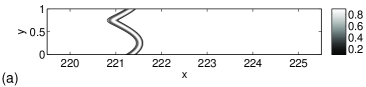
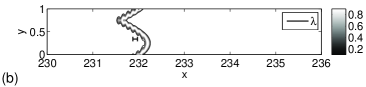
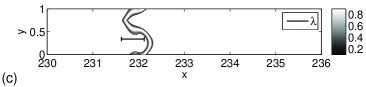
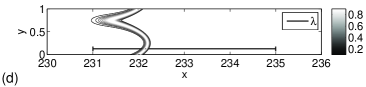
Figure 2: Snapshot of $4\theta(1-\theta)$ for a fixed Peclet number ($Pe=100$) and for Damköhler number $Da=100$. Panel (a) refers to a incompressible simulation ($\epsilon=0$) while for the others $\epsilon=0.5$. For the compressible tests the characteristic length $\lambda$ is set to be approximately lower (panel (b), $\lambda=0.1$), between (panel (c), $\lambda=0.5$) or greater (panel (d), $\lambda=4$) than the two thicknesses $\Delta$ and $\delta$.

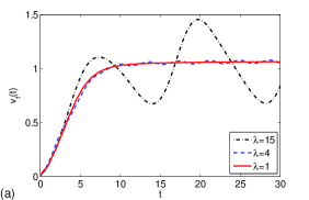
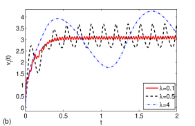
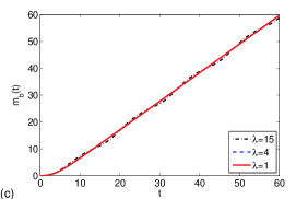
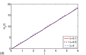
Figure 3: (Color online) Front speed and burnt mass ($m_{b}(t)=\int_{0}^{t}v_{f}(t)\leavevmode\nobreak\ dt$) as function of time for a fixed $Pe=100$, two different Damköhler ($Da=1$ in panel: a,c ; $Da=100$ in panel: b,d) and different $\lambda$.

In order to quantitatively characterize the effect of compressibility, we vary both the parameter $\epsilon$ and $Da$, with a fixed Peclet number. For this purpose, it is convenient to define the percentage difference of the mean asymptotic front speed between the compressible and the incompressible case as follow:

$$\Delta v_{\%}=100\leavevmode\nobreak\ \frac{v-v^{0}}{v^{0}}$$ (III.5)

where $v^{0}$ is the asymptotic bulk burning rate, as defined in (III.4), for the incompressible case ($\epsilon=0$). Results are shown in Figure 4.
In general, in the regimes investigated here, we observe that the presence of compressibility can slightly improve the process of reaction and the effects grow by increasing both $\epsilon$ and $Da$. For a fixed characteristic reaction rate (see Figure 4.a), numerical simulations suggest a power (quadratic) law of the velocity enhancement as a function of the parameter $\epsilon$

$$\Delta v_{\%}\sim\epsilon^{2}.$$ (III.6)

Instead, the dependence on Damköhler is much slower. As shown in Figure 4.b the parameter $\Delta v_{\%}$ is always positive an it grows following (approximately) a logarithmic law:

$$\Delta v_{\%}\sim a\ln(Da)+b$$ (III.7)

where $a$ and $b$ may depend on $\epsilon$. Therefore even in the case of very strong compressibility ($\epsilon=0.5$) and very fast reaction ($\alpha=1000$) the difference never exceeds a modest $6\%$.

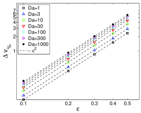
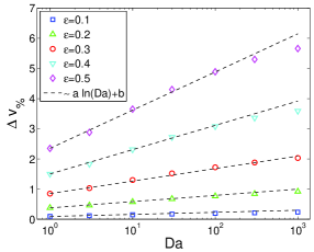
Figure 4: (Color online) Comparison of the front speed between compressible and incompressible shear flow for a fixed Peclet number ($Pe=100$) at different compressibility magnitude $\epsilon$ (on the left) and for different Damköhler (on the right).

The effect of compressible wave perturbations appears therefore to be: i) wrinkling; ii) second-order enhancement.

IV Compressible cellular flow

We discuss now the case of cellular flows, i.e., 2D steady flows of amplitude $U_{0}$ composed by counter-rotating vortex of dimension $L/2$. The compressibility is imposed in the following way:

$$\rho(x,y) =\rho_{0}C(x,y)$$ (IV.1)

$$\bar{u}(x,y) =\left(\frac{U_{0}\sin\left(\frac{2\pi y}{L}\right)\cos\left(\frac{2\pi y}{L}\right)}{C(x,y)},\frac{-U_{0}\cos\left(\frac{2\pi y}{L}\right)\sin\left(\frac{2\pi y}{L}\right)}{C(x,y)}\right)$$ (IV.2)

We choose two different shapes for $C(x,y)$. In the first, that we call (a) case, the density of the mixture is higher in the centre of the vortex:

$$C(x,y)=1+\epsilon\left(\left|\sin\left(\frac{2\pi x}{L}\right)\sin\left(\frac{2\pi y}{L}\right)\right|-\frac{4}{\pi^{2}}\right)$$ (IV.3)

In the second, that we call (b) case, the density is higher in the periphery of the vortex:

$$C(x,y)=1-\epsilon\left(\left|\sin\left(\frac{2\pi x}{L}\right)\sin\left(\frac{2\pi y}{L}\right)\right|-\frac{4}{\pi^{2}}\right)$$ (IV.4)

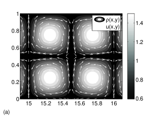
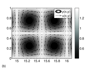
Figure 5: Compressible Cellular flow : (a) the density is higher in the centre of the vortex. (b) The density is higher in the outer region.

The two different configurations are shown in Figure 5. The constant factor $\frac{4}{\pi^{2}}$ has been introduced in order to have a density perturbation which is zero in average. As in the case of the shear flow, we study the dependence of the dynamics on the compressibility intensity $\epsilon$ and Damköhler number in the more realistic case of fixed high Peclet number.

We will consider a wider range of Damköhler exploring the regimes at $Da\ll 1$, $Da\approx 1$ and $Da\gg 1$. Nevertheless we will remain in regimes $PeDa>1$ which means that the characteristic diffusion time is always larger than the reaction time. Unlike the shear flow, in the cellular flow $\Delta v_{\%}$ does not show a monotonic dependence neither on $\epsilon$ nor on $Da$, as it can be seen from Figure 6.

Such a feature has been observed also for other configurations of $C(x,y)$ (simulations not shown here) confirming that the non monotonic behaviour of $\Delta v_{\%}$ is related to the whirling geometry of the flow rather than to the choice of the density perturbation. In the slow reaction regime ($Da\ll 1$) it can be seen in Fig. 6 an almost Damköhler-indipendent behaviour of $\Delta v_{\%}$ in both cases (a) and (b). On the other hand, in a middle range of Damköhler where the combined effect of advection and reaction is more intriguing, the two flow configurations show opposite trends for $\Delta v_{\%}$, the reaction is faster, when the density is higher in the centre (case (a)), whereas it is slower when the perturbation is at the periphery (case (b)). Such a behaviour is not surprising, since the interplay between reaction and diffusion in the presence of closed streamlines can lead to a non trivial behaviour also in the case of uncompressible flow acvv1 , and the presence of variations in the density of the flow can act in a very non intuitive way.

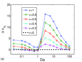
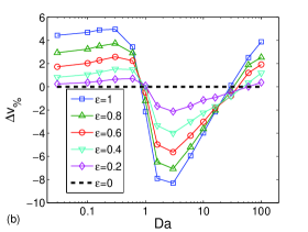
Figure 6: (Color online) (a,b) Percentage difference between compressible and incompressible test case of the mean asymptotic bulk burning rate. $1/Pe=0.003$. In panel $(a)$ the density of the fluid is higher in the centre of the vortexes while in panel $(b)$ the density is higher in the periphery.

V Conclusions

We have studied the propagation of fronts through an advection-diffusion-reaction equation where the nonlinear reaction term is given by the classical FKPP source term. The advective flow is generated by an imposed field which is perturbed by compressible waves. The compressibility is controlled by the parameter $\epsilon$. Two velocity fields have been considered: a shear-flow and a cellular one.

In the considered flows, the front can be strongly affected by compressibility and the compressibility field forces a strong localization of density, but the quantitative differences with respect to the incompressible model appear modest (of the order of some percent). On the basis of previous studies, we do not think that the presence of chaos (turbulent fluctuations) should change much the scenario ctvv .

Some comments are in order to discuss the apparent difference of the behaviour of $\Delta v_{\%}$ in the cases of shear flow and cellular flow (see Figs. 4 and 6). The stream lines in the two cases are very different: namely open and closed, respectively. In the shear flow, the effect of compressibility on the front propagation is only slightly modified with respect to the uncompressible case, since the front is mainly driven by the stream. On the other hand, closed streamlines trigger entangled mechanisms between reaction and diffusion, that, coupled with the compressibility generate highly non trivial features. An example of this complicated behaviour can be found in the non monotonic dependence of $\Delta v_{\%}$ by the Damköhler number, or in the well apparent difference between cases (a) and (b) of the cellular flows here considered.

Finally, it is interesting to note that a similar model has been recently used for the study of population dynamics in turbulent flows benzi :

$$\frac{\partial{C}}{\partial t}+{\bf\nabla}\cdot({\bf u}C)=D_{0}\nabla^{2}C+\mu C(1-C)$$ (V.1)

where the scalar $C({\bf x},t)$ is the concentration of a population benzi , which is the equivalent of our $\rho\theta$ in Eq. (II.5). When ${\nabla}\cdot{\bf u}\neq 0$, clustering of the population near compression regions $({\nabla}\cdot{\bf u}<0)$ is observed. In those regions, the concentration can take values greater then one and reaction rate on Eq. (V.1) can be negative, so that the scalar $C({\bf x},t)$ is not a fractional parameter. Within this model, authors linked changes in the overall carrying capacity of the ecosystem (i.e. the density of biological mass of the system) to the compressibility and its effect of localisation. Yet, present results show that the change of the carrying capacity is not due to density localisation, but rather to the choice of a different reaction term, which allows negative rate in high density zones. Indeed, in the present work we have a strong density localisation but our FKPP model for a fractional parameter does not allow negative rate. The results is that the average carrying capacity does not change even in presence of compressible flows. The analysis of present results for the Lagrangian displacement of passive reactive tracers and irreversible reaction dynamics is ongoing.

VI Acknowledgements

We would like to thank Dr Guillaume Legros, P. Perlekar and Dr Roger Prud’homme for fruitful discussions.

References

- [1] J. Xin. Front propagation in heterogeneous media. SIAM Review, 42:161, 2000.
- [2] P Constantin, A Kiselev, A Oberman, and L Ryzhik. Bulk burning rate in¶ passive–reactive diffusion. Archive for rational mechanics, Jan 2000.
- [3] D. Vergni and A. Vulpiani. Front propagation in stirred media. Milan Journal of Mathematics, 79:497, 2012.
- [4] F. A. Williams. Combustion Theory. Benjamin-Cummings, Menlo Park, 1985.
- [5] J. Ross, S. C. Müller, and C. Vidal. Chemical waves. Science, 240:460, 1988.
- [6] I. R. Epstein. The consequences of imperfect mixing in autocatalytic chemical and biological systems. Nature, 374:231, 1995.
- [7] E. R. Abraham. The generation of plankton patchiness by turbulent stirring. Nature, 391:577, 1998.
- [8] E. R. Abraham, C. S Law, P. W. Boyd PW, S. J Lavender, M. T Maldonado, and A. R. Bowie. Importance of stirring in the development of an iron-fertilized phytoplankton bloom. Nature, 407:727, 2000.
- [9] J.S. Guasto, R. Rusconi, and R. Stocker. Fluid mechanics of planktonic microorganisms. Annual Review of Fluid Mechanics, 44:373–400, 2012.
- [10] KS Korolev, M. Avlund, O. Hallatschek, and D.R. Nelson. Genetic demixing and evolution in linear stepping stone models. Reviews of Modern Physics, 82(2):1691, 2010.
- [11] F. d Ovidio, S. De Monte, S. Alvain, Y. Dandonneau, and M. Lévy. Fluid dynamical niches of phytoplankton types. Proceedings of the National Academy of Sciences, 107(43):18366–18370, 2010.
- [12] A. N. Kolmogorov, I. G. Petrovskii, and N. S. Piskunov. Study of the diffusion equation with growth of the quantity of matter and its application to a biology problem. Moscow Univ Bull. Math, 1:1, 1937.
- [13] R. A. Fischer. The wave of advance of advantageous genes. Ann. Eugenics, 7:355, 1937.
- [14] N. Peters. Turbulent combustion. Cambridge University Press, 2000.
- [15] R. Prud’homme. Flows of reactive fluids. Springer, 2010.
- [16] T. Poinsot and D. Veynante. Theoretical and numerical combustion. RT Edwards, Inc., 2005.
- [17] N. Vladimirova and R. Rosner. Model flames in the boussinesq limit: the effects of feedback. Physical Review E, 67(6):066305, 2003.
- [18] B. Audoly, H. Berestycki, and Y. Pomeau. Réaction diffusion en écoulement stationnaire rapide. Comptes Rendus de l’Academie des Sciences Series IIB Mechanics Physics Astronomy, 328(3):255–262, 2000.
- [19] N. Vladimirova, P. Constantin, A. Kiselev, O. Ruchayskiy, and L. Ryzhik. Flame enhancement and quenching in fluid flows. Combust. Theory Modelling, 7(3):487–508, 2003.
- [20] M. Abel, M. Cencini, D. Vergni, and A. Vulpiani. Front speed enhancement in cellular flows. Chaos, 12(2):481, 2002.
- [21] M. Cencini, A. Torcini, D. Vergni, and A. Vulpiani. Thin front propagation in steady and unsteady cellular flows. Phys Fluids, 2003.
- [22] M. Abel, A. Celani, D. Vergni, and A. Vulpiani. Front propagation in laminar flows. Physical Review E, 64(4):046307, 2001.
- [23] P. Constantin, J.M. Roquejoffre, L. Ryzhik, and N. Vladimirova. Propagation and quenching in a reactive burgers–boussinesq system. Nonlinearity, 21(2):221, 2008.
- [24] P. Perlekar, R. Benzi, D.R. Nelson, and F. Toschi. Population dynamics at high reynolds number. Physical Review Letters, 105(14):144501, 2010.
- [25] DM Lewis and TJ Pedley. Planktonic contact rates in homogeneous isotropic turbulence: theoretical predictions and kinematic simulations. Journal of Theoretical Biology, 205(3):377–408, 2000.
- [26] J.P. Minier and E. Peirano. The pdf approach to turbulent polydispersed two-phase flows. Physics Reports, 352(1):1–214, 2001.
- [27] G. Falkovich, K. Gawedzki, and M. Vergassola. Particles and fields in fluid turbulence. Reviews of Modern Physics, 73(4):913, 2001.
- [28] J. Bec, L. Biferale, M. Cencini, A. Lanotte, S. Musacchio, and F. Toschi. Heavy particle concentration in turbulence at dissipative and inertial scales. Physical Review Letters, 98(8):84502, 2007.
- [29] N. Vladimirova, V.G. Weirs, and L. Ryzhik. Flame capturing with an advection–reaction–diffusion model. Combustion Theory and Modelling, 10(5):727–747, 2006.